Powertrain modelling for engine stop start dynamics and control of micro/mild hybrid construction machines

Original citation:

Dinh, Quang Truong, Marco, James, Greenwood, David, Harper, L. and Corrochano, D.. (2017) Powertrain modelling for engine stop-start dynamics and control of micro/mild hybrid construction machines. Proceedings of the Institution of Mechanical Engineers, Part K: Journal of Multi-body Dynamics, 231 (3). pp. 439-456.

Permanent WRAP URL:

http://wrap.warwick.ac.uk/88017

Copyright and reuse:

The Warwick Research Archive Portal (WRAP) makes this work by researchers of the University of Warwick available open access under the following conditions. Copyright © and all moral rights to the version of the paper presented here belong to the individual author(s) and/or other copyright owners. To the extent reasonable and practicable the material made available in WRAP has been checked for eligibility before being made available.

Copies of full items can be used for personal research or study, educational, or not-for profit purposes without prior permission or charge. Provided that the authors, title and full bibliographic details are credited, a hyperlink and/or URL is given for the original metadata page and the content is not changed in any way.

Publisher’s statement:

Dinh, Quang Truong, Marco, James, Greenwood, David, Harper, L. and Corrochano, D.. (2017) Powertrain modelling for engine stop-start dynamics and control of micro/mild hybrid construction machines. Proceedings of the Institution of Mechanical Engineers, Part K: Journal of Multi-body Dynamics, 231 (3). pp. 439-456. Copyright © 2017 The Authors

Reprinted by permission of SAGE Publicationshttps://doi.org/10.1177/1464419317709894

A note on versions:

The version presented here may differ from the published version or, version of record, if you wish to cite this item you are advised to consult the publisher’s version. Please see the ‘permanent WRAP url’ above for details on accessing the published version and note that access may require a subscription.

Powertrain modelling for engine stop-start dynamics and control of

micro/mild hybrid construction machines

T.Q. Dinh1,*_{, J. Marco}1_{, D. Greenwood}1_{, L. Harper}2_{, D. Corrochano}2

1_{Warwick Manufacturing Group (WMG), University of Warwick, Coventry CV4 7AL, UK;}

[email protected]; [email protected]; [email protected]

2_{JCB, Rocester, Staffordshire, ST14 5JP, UK; [email protected]; [email protected]}

*Correspondence: [email protected]; Tel.: +44-2476-574902

Abstract

Engine stop-start control is considered as the key technology for micro/mild hybridisation of vehicles and machines. To utilize this concept, especially for construction machines, the engine is desired to be started in such a way that the operator discomfort can be minimized. To address this issue, this paper aims to develop a simple powertrain modelling approach for engine stop-start dynamic analysis and an advanced engine start control scheme newly applicable for micro/mild hybrid construction machines. First, a powertrain model of a generic construction machine is mathematically developed in a general form which allows to investigate the transient responses of the system during the engine cranking process. Second, a simple parameterisation procedure with a minimum set of data required to characterise the dynamic model is presented. Third, a model-based adaptive controller is designed for the starter to crank the engine quickly and smoothly without the need of fuel injection while the critical problems of machine noise, vibration and harshness can be eliminated. Finally, the advantages and effectiveness of the proposed modelling and control approaches have been validated through numerical simulations. The results imply that with the limited data set for training, the developed model works better than a high fidelity model built in AMESim while the adaptive controller can guarantee the desired cranking performance.

Keywords

1. Introduction

As reporting from the Environmental Protection Agency, construction industry is the third most significant sector just behind oil and gas and chemical manufacturing in terms of having influence on the greenhouse effect. Additionally, energy crisis becomes more serious in recent years while fuel consumption of heavy off-road equipment accounts for a significant portion of total global fuel usage. Thus, improving fuel efficiency of construction equipment without sacrificing the working capability is one of the key factors for creating a clean environment and saving energy.

There have been much research effort on hybridization technologies in terms of fuel economy and environmental impacts for various applications ranging from transportation to construction equipment. In the construction site, although full hybrid electric systems1 _{could offer many}

advantages over traditional configurations, they suffer from a comparatively high cost for the implementations, reliability and consumer acceptability. Recently, micro/mild hybridisation (MMH) has been widely used for modern vehicles due to its advantages, including high fuel efficiency, low emission and especially, low cost and easy installation regardless of drivetrain configuration.2-4 _{During operation of a machine, such as excavator, wheel loader, forklift or}

telescopic handler, and particularly at the times of reduced workloads (as load lowering) or task waiting (as load holding), less than full engine power is required to enhance an effective performance. Such periods of reduced workloads present good opportunities to improve the fuel efficiency as well as to reduce the machine noise, vibration and pollution. Therefore, MMH can be considered as an affordable solution for construction machinery.

For a micro/mild hybrid vehicle, one of the key functions affecting the overall performance is known as engine stop-start (ESS) operation. There is a number of studies on ESS control for both conventional vehicles5_{and hybrid vehicles.}1,6_{Although the engine performance could be improved}

peak compression torque and machine noise, vibration and harshness (NVH) problem. Hence in order to utilize the ESS control for micro/mild hybrid machines, two important tasks which need to be addressed are to determine states of the engine to switch it into idle mode or turn it off and, to design an engine start controller to start the engine quickly and smoothly to reduce impacts of NVH on the driver comfort. Several relevant studies on automatic engine idle detection and control have been proposed.7,8_{However, to the best of the authors’ knowledge, a research on how to design}

proficiently the start controller for the ESS for the construction sector has not been stated.

Therefore, this paper focuses on the development of a simple powertrain modelling approach and an advanced engine start controller for a generic micro/mild hybrid construction machine. First, the powertrain mathematical model of a traditional excavator is generally conducted to investigate the system transient response during the engine cranking process. Here, the powertrain model is built as the combination of sub-models, including transmission sub-models, engine sub-model, and electrical components’ sub-models. Second, a simple optimization procedure with a limited data requirement is introduced to parameterise the model to represent the start-up performance. Third, a model-based adaptive controller is designed as the combination of an inverse model, which is derived from the optimized model, and a proportional-integral (PI)-based adaptive controller to drive the starter to enhance the quick and smooth engine start. Finally, a physical model is built in AMESim and then, embedded into MATLAB/Simulink to perform a comparative study of the engine performance estimation with the proposed mathematical model. Numerical simulations are carried out to evaluate the capability of the proposed modelling and control methods.

2. Powertrain architecture and problem statement

[image:5.595.121.506.194.378.2]

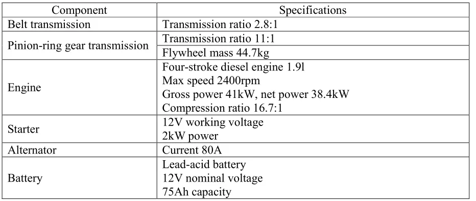
a hydrostatic transmission (HST) which are connected to the engine output shaft through a clutch. These parts also can be simplified as an external load with adjustable inertia. In this study, the powertrain of a research excavator from JCB is used for the model development and analysis. Specifications of the main components of this powertrain are given in Table 1.

Figure 1.Powertrain configuration of a generic construction machine.

Table 1.Specifications of the powertrain’s main components.

Component Specifications

Belt transmission Transmission ratio 2.8:1

Pinion-ring gear transmission Transmission ratio 11:1 Flywheel mass 44.7kg

Engine

Four-stroke diesel engine 1.9l Max speed 2400rpm

Gross power 41kW, net power 38.4kW Compression ratio 16.7:1

Starter 12V working voltage_{2kW power}

Alternator Current 80A

Battery

Lead-acid battery 12V nominal voltage 75Ah capacity

[image:5.595.81.547.433.630.2]

around 850 to 950rpm) while the starter is disengaged and its power is cut off. By this way and due to the use of larger engine sizes compared to passenger vehicles, the cranking time of a construction machine is normally longer while there is more significant impact of NVH on the driver. To address the existing problems, the advanced cranking approach has been developed. Herein, the conventional starter is replaced by an electric motor with a larger power capable of cranking the engine directly from zero speed to the idle speed without the injection.

In order to theoretically investigate the transient response of the powertrain, it is necessary to develop a model that accounts for both the engine, starter and alternator dynamics and their interactions. Lots of activities in designing a complete powertrain/engine model have been presented in the literature. However, high-order nonlinear models are sophisticated and computationally demanding. These models normally require an extensive amount of experimental data and a complex training process which subsequently limit their applicability.6,9,10_Furthermore

to start the engine more quickly with less NVH, a model-based control is indispensable for the starter. Therefore, there is a demand on conducting a control-oriented model for both the powertrain dynamic analysis and engine start control. Due to the focus on engine start performance, dynamics of the clutch at the engine output shaft are not considered and, then, this clutch and external load at the engine output shaft can be neglected or approximated as a small constant load rigidly connected to the engine output shaft.

3. Powertrain dynamic model design and parameterisation

3.1. Powertrain dynamic model

Based on the powertrain configuration introduced in the previous section, the powertrain dynamic model is built as the combination of following sub-models:

 Belt transmission sub-model

 Pinion-ring gear transmission sub-model

 ICE sub-model

 Starter sub-model

3.1.1. Belt transmission sub-model

The alternator is driven by the engine via the belt transmission. By taking into account the axial deformability of the branches, a lumped parameter model of a spring-damper system is commonly used to represent the belt transmission.11,12 _{From this assumption, the belt transmission can be}

modelled via Lagrange equations as:

, 1, 2

Energy Energy Energy Energy Energy

i i i i i

T T P D W

d i dt                   _  _{  }

  (1)

where:



2 2



1 1 2 2 1

2

Energy

T  J  J  (2)





2

1 1 2 2

Energy B

P  k R R  (3)





2

1 1 2 2

Energy B

D  c R  R  (4)

1 1 2 2

Energy

W     (5)

By replacing equations (2)-(5) into equation (1), the belt transmission is represented by

















1

1 1 1 1 2 2 1 1 1 2 2 1

2

2 2 1 1 2 2 2 1 1 2 2 2

2

2

2

2

B B

B B

d

J

k R R

R

c R R

R

dt

d

J

k R R

R

c R R

R

dt



_

_

_

_

_



_

_

_

_

_



_

_

_

_

_







_

_

_

_

_{ }



(6)

3.1.2. Pinion-ring gear transmission sub-model

where:

1,IF:SOLisenergized

0,

SOL

ELSE



_{ }





(8)

0,IF:

1,

OR

sat

S S

C

ELSE

 



_{ }







(9)

3.1.3. ICE sub-model

For the engine stop-start analysis and control, the ICE sub-model is developed for two cranking cases, using starter (without injection) and using injectors (without starter activation). Without loss of generality, the below mathematical relations are derived to build a dynamic model of a single cylinder of the ICE. Then based on the number of cylinders of the ICE, their firing order and phase differences, the ICE sub-model can be then constructed as the set of cylinder models.

a) Engine dynamics during cranking with only starter

The engine can be modelled as a combination of intake manifold filling dynamics, reciprocating inertia induced by the piston, and engine friction dynamics. For a defined angular position of the engine,_E, the engine torque can be computed as:13

E ind iner fr

    (10)

where:

 _indcan be derived using the geometric design of the crank-slider mechanism of each cylinder:





sin_{2 2}cos ₂

sin

/ sin

E E

ind crank pis cyl amb E

rod crank E

R A P P

L R

 

 



 

 

  

 _ 

 

(11)

cyl cyl cyl

E cyl E

dP P dV

d  V d (12)







_{2 2 2}



1/2

0 0

1

1 / 1 cos / sin

2

cyl cyl cyl com rod crank E rod crank E

V V  V C  _L R     L R   _

 _inercan be computed as:

2 2 2

sin cos sin

/ sin

E E

iner crank iner E

rod crank E

R F L R             _    (14) 2 2 2 pis pis

iner iner E E

E E

dx d x

F M

d  d 

 

 _  _

 

  ₍₁₅₎



_{2 2 2}



1/2

1 cos / sin

pis rod crank E rod crank E

x L R _ 



 L R 



_

  (16)

 _fris computed as:

2

0 1 2 E 3 E

fr fr fr cyl fr fr

d d

k P k k dt dt

 

     _ _

  (17)

, 1, 2, 3

i i i

fr fr fr

k a b T i (18)

Based on equations from (10) to (18), the engine torque can be computed with respect to the cranking speed.

b) Engine dynamics during cranking using fuel injectors

In case of activating the injection, the in-cylinder pressure is derived from the analysis of thermodynamic processes. For a closed system, the first law of thermodynamics is written as10,13

in loss

dQ dQ dW dU (19)

cyl cyl

dW P dV (20)

For an ideal gas, following law is obtained:

cyl cyl g g g

P V n R T (21)

or,

cyl cyl cyl cyl g g g

dP V P dV n R dT (22)

Similarly, the change in internal energy of an ideal gas can be derived by

g vg g g vg g

dU n dC T n C dT (23)





vg

cyl cyl cyl cyl g vg g

g C

dU dP V P dV n dC T

R

   (24)

By substituting equations (20) and (24) into equation (19), following relation is obtained:

cyl vg cyl cyl vg

in loss

cyl cyl cyl g g

E E E g E E E

dV C dP dV dC

dQ dQ

P V P n T

d d d R d d d

 

   _  _

  (25)

For an ideal gas, one has:

1 g

vg R

C   (26)

By considering the heat capacity at constant volume and equations (25) and (26), the in-cylinder pressure in equation (12) can be derived from a full from as follows:

1

cyl cyl cyl in loss

E cyl E cyl E E

dP P dV dQ dQ

d V d V d d

            _  _

  (27)

The combustion heat release can be calculated as

in b

f f

E E

dQ

dx

m LHV

d





d



(28)

where, xbcan be approximately represented by Wiebe functions13,14counting for the premix and diffusion phases:

1 ₁

0 ₀

0 0

1 1

m p _md

E Ep

p _p d E Ed

d

Ep Ed

m _a m

a

p E Ep

b d E Ed

p p d d

E Ep Ep Ed Ed

m

dx m

k a e k a e

d                 _        _{ } _   _               _ _{ } _  _  _      (29)

here,kp,kdare determined as follows:10,15

1 , 1

b

p c d p

ignd

k a  k k



    (30)

here,a,bandcare within ranges13_{: [0.8, 0.95], [0.25, 0.45] and [0.25, 0.5], respectively; and}

ignd



can be derived using the Arrhenius-based correlation algorithm:16

2100 0.2 1.02

2.4 Tg

ignd Pcyl e

The heat losses can be computed using the Annand correlation:

 





g E g g w

loss

E E

A h T T

dQ d



 



 (32)

where,hgis derived by the Woschni model based on the steady turbulent heat transfer13,17:

0.2 0.8 0.546 0.8 129.8

g pis cyl g g

h _ D P T u ₍₃₃₎

whereugis calculated during the expansion process as



*



2.285 cyl gr

g pis g cyl cyl

r r

V T

u u c P P

PV

   (34)

where *

cyl

P is the in-cylinder pressure when the piston is at the same position and there is no

combustion (derived by equation (12)).

30

E cyl pis

n S

u



(35)

The four-stroke engine in this study can be then modelled as the combination of four cylinder models representing by the equations (10) to (35). Here, the firing order is 1-3-4-2 while the phase shift between these cylinders is 180-degree and the initial angle of the fist cylinder is -270 degrees.

c) Simple engine control unit (ECU) logic for injection control

Once the ICE speed reaches to the low idle level (using the starter), the fuel injectors are activated after a short delay time (_injd) defined by the manufacturer. A simple ECU control logic is needed

to command the injectors to rise the ICE speed to the normal idle level. This control action can be simply represented by a proportional-integral-derivative (PID) algorithm. By considering the ICE speed tracking error,e_, the fuel injection can be controlled by the followings:

0

f f f

f P I D

cmd

E E

m

m

m

de

m K e K e dt K

dt

e



 











 









wherem_f0is computed based on the engine fuel consumption map while m_f is derived by the PID controller.

3.1.4. Starter sub-model

Figure 2.Representative circuit of DC motor.

A representative circuit of a DC motor can be described as in Figure 2. Based on this circuit and the Kirchhoff’s voltage law, the following relation can be given:

S

S S S S S S

dI

V I R L k

dt 

   (37)

The motor torque can be computed as

S k I S

  (38)

3.1.5. Alternator and battery sub-models

In order to complete the powertrain model, sub-models of the alternator and battery are necessary. Because the focus of this study is about engine start dynamics and control while the dynamic responses of the electrical components are very fast compared to the engine behaviour, they can be represented by using performance maps.

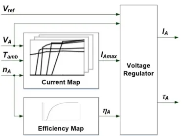
Using a performance map from the manufacturer, the alternator sub-model can be built with four inputs, the target regulation voltage (Vref), alternator voltage (VA), alternator speed (nA) and temperature (Tamb), and three outputs, the alternator output current (IA) and torque (_A), as depicted

[image:13.595.147.466.101.618.2] [image:13.595.220.406.103.242.2]

Figure 3.Alternator sub-model structure.

Figure 4.Complete powertrain model built in Simulink.

The battery is represented by a simple equivalent circuit model18_{and a performance map from}

BAT S A

I  I I (39)

0

BAT

BAT

dSoC I

dt  Q (40)

The terminate voltage is then calculated based on the battery performance map of the open circuit voltage andSoC.

Finally, by combining all the designed sub-models, the complete powertrain model is established in MATLAB/Simulink as displayed in Figure 4.

3.2. Model parameterisation

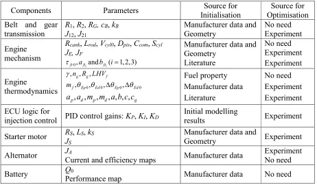
[image:14.595.82.544.417.687.2]

As the next step to develop the powertrain model, its decisive parameters need to be appropriately identified. A simple model identification approach is therefore introduced in this section. The key parameters as well as the sources for setting their initial values are listed in Table 2.

Table 2.Model parameters and sources for parameter setting and optimisation.

Components Parameters _{Initialisation}Source for _OptimisationSource for

Belt and gear transmission

R1,R2,RG, cB,kB

J12,J21

Manufacturer data and Geometry

No need Experiment

Engine mechanism

Rcank,Lrod,Vcyl0,Dpis,Ccom,Scyl

JE, JF

0, iand i( 1,2,3)

fr afr bfr i

 

Manufacturer data and Geometry

Literature

No need Experiment Experiment

Engine

thermodynamics

, ,n R LHVg g, f



0 0 0 0

, , , ,

f Ep Ed Ep Ed

m    

, , , , , , ,

p d p d g

a a m m a b c c

Fuel property Manufacturer data Literature

No need Experiment Experiment ECU logic for

injection control PID control gains:KP,KI,KD

Initial modelling

results Experiment

Starter motor RS,LS,kS JS

Manufacturer data and

Geometry Experiment

Alternator J_{Current and efficiency maps}A Manufacturer data Experiment_{No need}

By looking at this table, it can be seen that most of the model parameters can be obtained through the manufacturer data, fuel specifications and geometric designs. The remained parameters, including friction, inertia, thermodynamic and motor parameters, are initialized using the literatures while the PID control gains are designed for the powertrain model using the Ziegler-Nichols method19_{. Next, these sets of parameters are optimized through a proper data training}

[image:15.595.83.544.254.555.2]

process.

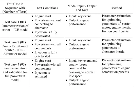
Table 3.Procedure and method for powertrain model optimization.

Test Case in Sequence with (Number of Tests)

Test Conditions Model Input / Output_{and Data} Method

Test case 1 (01) Parameterization of starter – ICE model

 Engine start

 Powertrain without connecting to alternator

 Injection is fully deactivated

 Input: key event

 Output: engine performance

Parameter estimation for optimizing parameters of starter motor, engine inertia, friction coefficients

Test case 2 (01) Parameterization of

Starter – ICE – Alternator model

 Engine start

 Powertrain with all components

 Injection is fully deactivated

 Input: key event

 Output: engine performance

Parameter estimation for optimizing parameters of alternator inertia

Test case 3 (03) Parameterization and validation for

full powertrain model

 Engine start

 Powertrain with all components

 Injection is activated

 Input: key event, and engine torque

command for cranking to normal idle speed

 Output: engine performance

Parameter estimation for optimizing parameters of engine combustion process

Here, nonlinear least square-based parameter estimation approach is employed to characterise the model based on a series of experiments on the actual powertrain. Only three test cases are required to support the optimisation. The definition of these test cases as well as the test procedure is presented in Table 3. Herein, the experiments are the typical ICE cranking tests on the research excavator in the normal working temperature, around 25o_{C. The starter is firstly enabled to drive}

4. Engine start controller

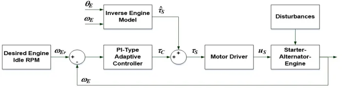
[image:16.595.138.488.206.297.2]

In order to start the engine smoothly and quickly without the fuel injection, the engine start controller is proposed as described in Figure 5. This controller contains two modules, the inverse powertrain model and the PI-based adaptive controller.

Figure 5.Proposed model-based control architecture for engine start.

From Section 3, the optimized model of the traditional powertrain could simulate well the system dynamics during the engine start-up. However for control applications, especially for engine start control, this complex model is redundant and hard to be utilized. Therefore, the powertrain model is firstly simplified in case the injection is deactivated and, then, the inverse model is created in which the model inputs are the ICE speed,_E, and crankshaft angle,_E, while

the output is the estimated torque command,ˆ_S, applied to the starter shaft. Hence, the inverse model is capable of reducing the influence of dynamic load torque on the starter.

Next, the PI-based adaptive controller is constructed to generate the compensative torque,_C, to deal with the system uncertainties, un-modelled dynamics and disturbances. This is then added to the estimated starter torque to produce the command,_S, for the starter to ensure that the engine can track the desired ICE speed well. This adaptive controller is built in a form of PI algorithm using a simple neural network of which the network weights are tuned online under a Lyapunov stability condition.

4.1. Inverse powertrain model

1 1

2

E

E S G L A

d

R

J

R

dt

R



 



 



 



_



_





(41)

Next, the ICE torque components in equation (10) are considered for a simplification. First, due to no injection during the cranking process, the indicate torque can be computed by the dynamic relations in equations (11) to (13). Second, it is known that the effect of reciprocating inertia torque,

iner

 , on the engine performance is significantly small, especially when comparing with the indicated torque,_ind.13_{As described in equations (11) and (14), these two factors have the similar}

phase and, therefore, impact of the inertia torque on the ICE output torque is very limited. In addition, for an engine with a number of similar cylinders arranged uniformly, these inertia torque components can be cancelled themselves. Hence, it is reasonable to eliminate the inertia torque,

iner

 , while computing the instantaneous ICE torque. Third, the friction torque can be calculated by

equation (17) in which the temperature-dependent parameters in equation (18) can be approximated as quasistatic terms. The reason is that the engine temperature is slowly varied compared to the short cranking process. Subsequently, depending on the temperature of the engine once it starts to be cranked, the friction parameters can be derived by equation (18) and kept constantly over the starting operation.

From the above analysis, equation (41) can be rewritten as

 

 

2 1

1 0 1 2 3

2

E

ind E fr fr cyl E fr E fr E L A S G

d

R

J

k P

k

k

R

dt

R



_{ }



_

_

_

_{  }



_





_







 

_







(42)

The inverse powertrain model represented by equation (42) can be used to compute the estimated torqueˆ_S to drive the starter.

4.2. PI-based adaptive controller

Here, the PI-type adaptive controller is suggested as a neural network which is generally built for a system with one control input,u, andnoutputs,y1_,y2_{, …,y}n_{, (in this case,uC;n=1). Define}

1 1

{ ,..., }

NN n

k k k

e  e e with i des i, act i,

k k k

two nodes, taggedPandI, following the PI algorithm, and an output layer to compute the control inputu.

Define

{ , }

w w

kPi kIi is the weight vector of the hidden nodes with respect to inputith, and

{ , }

P I

k k

w w

is the weight vector of the output layer. Therefore, the output from each hidden node is derived based on the PI algorithm:

1

1 1

:Node :Node

n

P Pi i

k i k k

n

I I Ii i

k k i k k

O w e P

O O w e I

  _  _     





(43)

And, the output from the network is obtained as:

 

NN NN P P I I

k k k k k k k

u  f O O w O w O (44)

4.2.1. Online training mechanism

To ensure the robust control performance, the back-propagation algorithm based on a Lyapunov stability condition is implemented to tune the network weights. Let’s define a cost function of the control errors as



  

1 1 2 2 , ,

1

2

n NN NNi

k _i k

NNi des i act i i

k k k k

E

E

E

y

y

e

 











(45)

By letting

{ , }

w w

_kP _kI to unit, the hidden weights can be online tuned for each step, (k+1)th_{, as}

follows:

1 , or

NN

ji ji ji k

k k k ji

k

E

w w j P I

where Piand Ii

k k

  are within (0,1]; the other factors in equation (46) are derived using partial

derivative of the function (45) with respect to each decisive parameter, chain rule method,20

equations (43) and (44):

, , 1 , 1 , or

NN n NNi act i

k k k k

ji act i ji

i

k k k k

act i n

i k i

k k

i k

E E y u

w y u w

y

e e j P I

u           _  _  _{ }  _      _{  }      





(47) , , , , 1 1

act i act i act i act i

k k k k

k k k k

y y y y

u u u u

 

  

 

   (48)

Additionally, in order to deal only with the system control errors, the influence of ratio between amplitudes of the system output and control input can be neglected. Consequently, equation (48)

can be simplified using sign function ( , ,

/ sign( / )

act i act i

k k k k

y u y u

     ). Hence, equation (47) can

be rewritten as

,

1

sign , or

NN n act i

i i k k k k ji i k k E y

e e j P I

w  u

   

 _{ }  _

 _  _

 

 _



_{ }  _ (49)

4.2.2. Lyapunov stability condition

The initial weights of the PI-based adaptive controller can be firstly derived based on a conventional PI controller which is designed using the Ziegler-Nichols method. These weights are then online regulated using the updating algorithm (46) to improve the control performance. In order to ensure the system robustness, a stability condition is introduced by the following theorem.

Theorem 1: By selecting properly the learning rates

  

_kPi

 

_kIi _kfor step (k+1)th_{to satisfy equation}



2



1 1

0.5

0

with

n i

k k k k

i

q NN q NN

n

k k k k

k Pi Pq Ii Iq

q k k k k

e F

F

e

E

e

E

F

w

w

w

w



 













 

_



_













(50)

Proof: by defining a Lyapunov function as equation (51), the change of this function is derived as equation (52)



_{, ,}



2

 

2

1 1

1

1

2

2

n n

NN des i act i i

k k k k

i i

V

y

y

e

 











(51)

   





  



2 2 1 1 1 2 1 1

1

2

1

,

2

n

NN i i

k k k

i n

i i i i i i

k k k k k k

i

V

e

e

e e

e

e

e

e

    













_

  

_

  









(52)

From the PI-based controller structure, one has:

1

i i

n

i k Pq k Iq

k Pq k Iq k

q k k

e

e

e

w

w

w

w











 

_







_











(53)

Terms



w

kPq

,



w

kIqare obtained from equation (46). By using the partial derivatives, selection of

Pj Pj

k k k

  





and definition of Fin equation (50), equation (53) becomes:

i

k k k

e



F

 

(54)

From equation (54), equation (52) is rewritten as

2 1 1 1 2 n NN i

k k k k k k

i

V 



e F F





 

  _  _

 



(55)

According to the Lyapunov stability theory,21 _{the tracking performance is guaranteed to be}

stable only if 1

0,

NN k

V

_

k

determined online based on the control errors. Hence for each working step, it is easy to select a

proper value of



k to make equation (50) satisfy. Therefore, the proof is completed.

5. Simulations and discussions

5.1. Powertrain model validation

In order to evaluate the capability of the designed powertrain model, a comparative study in engine cranking performance estimation has been carried out between this model (tagged as Model 1), another high fidelity model built using AMESim22_{and MATLAB/Simulink (tagged as Model 2),}

and the experimental results.

5.1.1. Model 2 design

Based on the powertrain configuration described through the previous sections, the Model 2 is built in AMESim as the combination of AMESim sub-models capable of representing the transmissions, ICE, starter, alternator and battery. This combined model is then packaged as a black-box model and embedded into Simulink environment as an S-function with a mask of all decisive parameters to support the model characterisation and validation.

a) AMESim sub-models of transmissions and load

The pinion-ring gear mechanism is modelled as a gear transmission connected to a controllable clutch. Additionally, the integrated flywheel is presented by a constant rotary load while all the friction losses through this transmission is presented by a friction mean effective pressure model (Figure 6(a)). By assuming that there is no extension or damage of the belt, the belt transmission model is a set of a two-input-one-output rotary node, a gear transmission with fixed ratio and a rotary spring-damper as in Figure 6(b). The external load at the engine output shaft can be represented by a constant small rotary load with another rotary spring-damper (Figure 6(c)).

From Starter Shaft

Clutch Control Signal

To Engine Shaft Flywheel Friction Losses Gear

Transmission

To Alternator Shaft

From

Engine Shaft Engine Final

Output Shaft Damping

Mechanism

Fixed Ratio Transmission

Damping Mechanism From Final

Output Shaft

External Loads

[image:22.595.234.395.104.178.2]

(c)

Figure 6.AMESim transmission and load sub-models: (a) Pinion-ring gear transmission; (b) Belt

transmission; (c) External load.

b) AMESim ICE sub-model

(a)

Intake &

Compressor Exhaust &Turbin

Exhaust Gas Recirculation (EGR)

Injection Mechanism

4-Cylinder Block

From Starter - Flywheel

To Final Output Shaft & Belt Transmission with Alternator Injection Control Signals (Mass Air Flow Signal to ECU) (Actual Torque Request

from ICE Speed Controller)

(b)

Figure 7.AMESim ICE sub-model: (a) Configuration; (b) Model.

[image:22.595.105.519.261.653.2]

By using the library of engine component models in AMESim, the engine physical model is generated as in Figure 7(b). The parameters set for this model is taken from Table 1, AMESim default setting values and the previous thermodynamic modelling study.10_{To simulate the engine}

transient behaviour, the model inputs can be listed as:

 Combustion cylinder: coolant temperature, temperature and pressure of the injected fuel, start of injection and injection duration

 Intake and exhaust mechanisms: intercooler control signal throttle control signal, variable geometry turbine position, engine torque request, engine speed

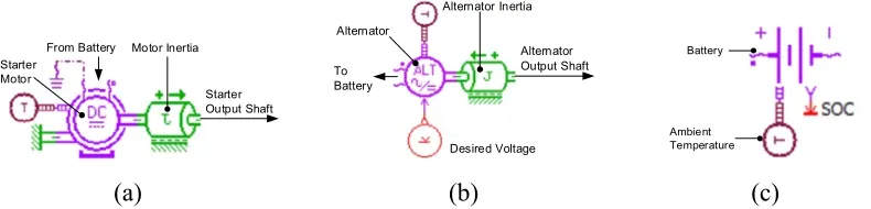
c) AMESim sub-models of starter, alternator and battery

By using AMESim, the equivalent electrical circuit of a direct current machine with permanent excitation is used to model the starter motor in which the inputs are temperature, supply voltage and rotational speed, and the outputs are current and load torque. Meanwhile, the alternator with DC output is represented as an average model of current generator with external voltage regulation. The model inputs are temperature, rotational speed, storage voltage and desired voltage while the outputs are torque and storage current. The battery is modelled by an equivalent electric circuit of variable voltage source and variable resistance which are the functions of the state of charge (SOC) and temperature. These component models are shown in Figure 8.

From Battery Motor Inertia

Starter Output Shaft Starter

Motor

Alternator Output Shaft Alternator Inertia

Alternator

To Battery

Desired Voltage

Battery

Ambient Temperature

[image:23.595.109.504.489.584.2]

(a) (b) (c)

Figure 8.Electric component models: (a) Starter motor; (b) Alternator; (c) Battery.

d) AMESim-Simulink control logics for Model 2

[image:24.595.95.528.105.328.2]

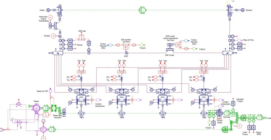
Figure 9.Complete Model 2 of a generic construction machine built in AMESim.

(to ECU)

(to Starter and ECU)

(Acceleration Signal to ECU)

(Engine Torque Command to ECU) (ICE Output Speed)

(a)

(Actual Torque Request to EGR)

(ICE Mode to ECU) (ICE Output Speed)

(ICE Torque Command)

(Starter ON Signal)

(Key ON Signal) (ICE Output Speed)

(b)

Control Signal to Injectors

(ICE Mode from ICE Speed Controller)

(ICE Output Speed)

(ICE Torque Command) (ICE Mass Air

Flow Signal)

(Starter Motor Desired Voltage) (ICE Output Speed) (Starter On/Off Signal)

(ICE Outputs: Speed & Crankshaft Angle)

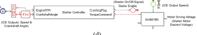
[image:25.595.143.485.107.168.2]

(d)

Figure 10. Model 2’s control logics: (a) Inputs; (b) Engine speed controller; (c) Engine control

unit; (d) Simulink-based starter control unit.

Next, the control logics are created to manage the model operation:

 Input signals: key On/Off event, pedal position, and engine torque command (Figure 10(a));

 Engine speed controller bases on the input signals and current engine speed to define the engine torque request and engine modes. Here, the engine operation is basically classified into four modes: engine start without/with injection, normal idle, and normal power (Figure 10 (b));

 Engine control unit uses the defined mode to control the combustion process with air flow, rail pressure and injection (Figure 10 (c));

 Starter control unit: with the traditional powertrain, there is only the direct connection between the motor and power supply models. An electric switch is used to turn on or off this motor. Conversely in the hybrid structure with ESS, the motor speed is controlled by the proposed controller, built in Simulink, via the inverter model (Figure 10 (d)).

As the last step, for the comparison with the Model 1, the complete Model 2 with its control logics is converted into the Simulink S-function capable of working independently without connecting to AMESim. By using this method, the same working environment and conditions can be applied to both the models 1 and 2.

5.1.2. Modelling results

(a)

[image:26.595.144.475.106.689.2]

(b)

[image:27.595.146.478.441.685.2]

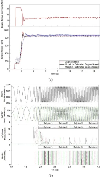
Subsequently, the model characterisation results were compared with the target performance as shown in Figure 11(a) while a model validation was performed as plotted in Figure 12. Herein, the first and second engine start experiments of the test case 3 for 15 seconds (Table 3, denoted as test cases 3-1 and 3-2) were in turn used to train and validate the models in which the input was the engine torque command and the output was the engine speed. The results indicate that both the models could estimate the speed profile. However, the modelling accuracy of Model 2 is low in some regions, especially during the cranking phase – the first three seconds. This is because the Model 2 is the high fidelity physical model based on the AMESim libraries. Therefore, there are a lots of model parameters (for example, parameters of the combustion cylinder, intake and exhaust mechanisms) need to be identified. With a limited number of experiments used for training, it is difficult to get the high modelling accuracy. Meanwhile, the goodness of fit between the Model 1 and the target profile is much higher than that of the Model 2 in both the cases. By using the developed mathematical modelling approach, the number of decisive parameters in the Model 1 is less than that of the Model 2 and, consequently, the better modelling accuracy is obtained by the Model 1 while using the same number of training data sets. The engine dynamics estimated by the trained Model 1 with respect to the test case 3-1 are demonstrated in Figure 11(b).

[image:28.595.149.480.109.350.2]

Figure 13.Comparative simulation results using powertrain models w.r.t. test case 3-3.

Another engine start test (test case 3-3) was carried out to validate the optimized models and, the comparison results were obtained as depicted in Figure 13. The results confirm that the proposed mathematical model always provided higher accuracy than the Model 2 in estimating the powertrain dynamics. Hence, this model is suitable for both engine modelling and start control development purpose.

5.2. Engine start control validation

In this section, numerical simulations on the developed model (Model 1) have been carried out to access the engine transient responses during start-up using the tradition cranking concept with the starter-injector and the proposed concept with only the controlled starter. Here, the desired cranking speed was set to 850rpm. With the suggested engine start method, the PI-based adaptive controller introduced in the previous section was used to manage the starter operation while the injection was fully cut off during this start-up phase.

[image:29.595.146.479.153.372.2]

NVH performance could be well managed and therefore, the driver comfort as well as fuel economy could be improved.

Figure 14.Comparison of simulated engine start performances using the traditional and proposed

cranking methods.

6. Conclusions

In this paper, the simple powertrain model and the advanced control method for starting engine of micro/mild hybrid construction machines have been firstly introduced. The powertrain dynamics could be well represented by the simple mathematical model which required only the small data set for the parameterisation. In addition, the main challenges to design the robust ESS control including fast response and reduction of NVH have been successfully addressed by the PI-based adaptive controller. The simulation results prove evidently both the superior capabilities of the designed model over the AMESim model and the suggested controller.

As a part of our research, a so-called prediction-based stop-start control (PSSC) technique for construction machines has been recently developed and successfully evaluated by means of simulations and hardware-in-the-loop tests using a simplified powertrain model23_{. Hence, one of}

Funding

This research is supported by Innovate UK through the Off-Highway Intelligent Power Management (OHIPM), Project Number: 49951-373148 in collaboration with the WMG Centre High Value Manufacturing (HVM), JCB and Pektron.

References

1. Liu D, Yu H and Zhang J. Multibody dynamics analysis for the coupled vibrations of a power split hybrid electric vehicle during the engine start transition.Proc IMechE Part K:

J Multi-body Dynamics2016; 230(4): 527–540.

2. Gao Y and Ehsani M. A Mild Hybrid Drive Train for 42 V Automotive Power System– Design, Control and Simulation.SAE International2002; 2002-01-1082:1-7.

3. Gupta S, Sharma R, Yuaraj KB, et al. Supervisory Control Strategy for Mild Hybrid System - A Model Based Approach.SAE International2013; 2013-01-0503:1-9.

4. Vallur AR, Khairate Y and Awate C. Prescriptive Modeling, Simulation and Performance Analysis of Mild Hybrid Vehicle and Component Optimization. SAE International2015; 2015-26-0010:1-17.

5. Robinette D and Powell M. Optimizing 12 Volt Start - Stop for Conventional Powertrains. SAE Int. J. Engines2011; 4(1): 850-860.

6. Kum D, Peng H and Bucknor NK. Control of Engine-Starts for Optimal Drivability of Parallel Hybrid Electric Vehicles.J. Dyn. Sys., Meas., Control2013; 135(2):1-10.

7. Park KS, Kim SI and Jeong HJ. Low Idle Control System of Construction Equipment and Automatic Control Method Thereof.US patent2013; US 2013/0289834 A1.

8. Frelich TA. Autoadaptive Engine Idle Speed Control. US patent2014; US 2014/0053801 A1.

9. Ipci D and Karabulut H. Thermodynamic and dynamic modeling of a single cylinder four stroke diesel engine.App. Math. Modelling2016; 40(5-6): 3925–3937.

11. Al-Dwairi AF and Al-Lubani SE. Modeling and dynamic analysis of a planetary mechanism with an elastic belt.Mechanism and Machine Theory2004; 39(4): 343-355. 12. Incerti G. A model for analysing the startup dynamics of a belt transmission driven by a

DC motor.Int. J. Mech., Aero., Ind., Mecha. and Manu. Eng.2014; 8(9): 1528-1533. 13. Rakopoulos CD and Giakoumis EG. Diesel engine transient operation: Principle of

operation and simulation analysis. Springer-Verlag London Limited: Springer, 2009. 14. Wiebe I. Halbempirische formel fuer die Verbrennungsgeschwindigkeit. Moscow: Verlag

der Akademie der Wissenschaften der UdSSR, 1956.

15. Watson N, Pilley AD, Marzouk M. A combustion correlation for diesel engine simulation.

SAE paper No. 8000291980.

16. Assanis DN, Filipi ZS, Fiveland SB, et al. A predictive ignition delay correlation under steady-state and transient operation of a direct injection diesel engine.ASME Trans, J Eng

Gas Turbines Power2003; 125:450–457.

17. Woschni G. A universally applicable equation for the instantaneous heat transfer coefficient in the internal combustion engine.SAE International1967: 670931.

18. Ambühl D.Energy Management Strategies for Hybrid Electric Vehicles. PhD thesis, ETH, Zurich, 2009.

19. Astrom KJ and Hagglund T.PID Controllers: Theory, Design and Tuning. North Carolina: Instrument Society of America, 1995.

20. Truong DQ and Ahn KK. Nonlinear black-box models and force-sensorless damping control for damping systems using magneto-rheological fluid dampers.Sens. Actuators A, Phys.2011; 167(2): 556-573.

21. Nikravesh SKY. Nonlinear Systems Stability Analysis: Lyapunov-Based Approach. Boca Raton: CRC Press - Taylor & Francis Group, 2013.

22. Truong DQ and Ahn KK. Force control for hydraulic load simulator using self-tuning grey predictor – fuzzy PID.J. of IFAC, Mechatronics2009, 19(2), 233-246.

Appendix

Notations

To avoid a large list, the parametric values are denoted by * and ** signs

* d

dt Derivative of * with respect to time

* **



 Partial derivative of * with respect to **

*

 A small increase in *

*

 A change of *

*E Variables related to internal combustion engine

*S Variables related to starter

*A Variables related to alternator

*F Variables related to flywheel

*L Variables related to external load

*B Variables related to belt transmission

*G Variables related to gear transmission

*g Variables related to gas

*BAT Variables related to battery

a,b,c Characteristic parameters of fractions of fuel,kp

ap,ad Combustion efficiency coefficients

1/2/3

fr

a ,bfr1/2/3 Component parameters of friction coefficients determined via practical tests

Apis Piston cross section area

 

g E

A  Instantaneous heat exchange surface inside combustion chamber of cylinder

cB Belt equivalent damping coefficient

cg Characteristic parameter of gas velocity

Ccom Geometric compression ratio

Cvg Heat capacity

DEnergy Rayleigh dissipation function of belt transmission mechanism

Dpis Piston diameter

i k

e Control error ofithoutput at time stepkth

e_ Engine speed tracking error

NN k

E Network’s cost function

Finer Inertia force

hg Convective heat transfer coefficient

IBAT Battery terminate current

IS Current of motor armature circuit

J Moment of inertia

J1 Sum of moment inertia of engine, 1stpulley (J12) and flywheel,J1=JE+J12+JF

kB Belt equivalent stiffness

1/2/3

fr

k Temperature-dependent friction coefficients

kp,kd Factions of fuel which burns in premixed and diffusion phases

kS,k_ Armature gain and torque constant of starter motor

KP/I/D PID control gains

Lrod Piston rod length

LHVf Fuel lower heating value

LS Armature conductance of starter motor

mf Mass of fuel injected per each cycle

0

f

m Average fuel mass injected per each cycle

mp,md Characteristic parameters of the Wiebe functions

Miner Equivalent mass of the parts including the reciprocating motion (piston, rod, connection pin)

nE Engine rotational speed

ng Amount of substance of gas (number of moles)

*

k

O Output from network’s node *that time stepkth

Pamb Ambient pressure

Pcyl In-cylinder pressure

PEnergy Potential energy of belt transmission mechanism

Pr Pressure at a reference condition

Qin Chemical energy of unburned fuel or combustion heat release

Qloss Heat losses transferred to the combustion chamber walls

QBAT0 Nominal battery capacity

R1,R2 Radii of pulleys 1 and 2

Rcrank Crank arm length

RG Transmission ratio of the pinion-ring gear system

Rg Ideal gas constant

RS Resistant load of starter motor

Scyl Cylinder stroke

SoC Battery state of charge

T Engine temperature

TEnergy Kinetic energy of belt transmission mechanism

Tg Gas temperature

Tgr Temperature at a reference condition

Tw Average temperature of heat exchange surface

uk Final output from network at time stepkth

ug Local average gas velocity

pis

u Mean cylinder velocity

U Internal energy of cylinder combustion chamber

VBAT Battery terminate voltage

Vcyl Instantaneous volume of cylinder

Vcyl0 Clearance volume of cylinder

Vr Displacement volume at a reference condition

VS Voltage of motor armature circuit

*i k

*

k

w Weight of network’s output with respect to node *that time stepkth

W Work done by working medium

WEnergy Work done by external factors of belt transmission mechanism

xb Fuel burning rate

xpis Piston displacement along cylinder bore

y* _{System *}th_output

 Coefficient of engine thermodynamics (specific heat ratio)

f m

 Fuel mass correction amount

,

Ep Ed

 

  Durations of premixed and diffusion phases

, OR

SOL C

  Activation functions of starter solenoid and over-running clutch

/

Pi Ii k



Learning rate of hidden weightith_{according to nodePorIat stepk}th

 Angular position

1, 2

  Angular positions of pulleys 1 and 2

0, 0

Ep Ed

  Crank angles at the start of premixed and diffusion phases of combustion

 Torque

1

 Sum of torques on the engine shaft, including external load torque (caused by the HST and HDT) and engine output torque,₁ _E _L

2

 Alternator torque, ₂   _A

C

 Starter compensative torque command

ind

 Engine indicate torque

iner

 Engine reciprocating inertia torque

fr

 Engine friction torque

fr

 Engine static friction torque

ignd

 Ignition delay

ˆ_S

 Estimated starter load torque



Overall fuel-air equivalent ratio

 Angular velocity

1, 2

  Angular velocities of pulleys 1 and 2

cmd E

 Commanded speed of engine

sat S