Efficient use of partially converged simulations in evolutionary optimization

warwick.ac.uk/lib-publications

Original citation:

Branke, Jürgen, Asafuddoula, M., Bhattacharjee, Kalyan Shankar and Ray, Tapabrata. (2016)

Efficient use of partially converged simulations in evolutionary optimization. IEEE

Transactions on Evolutionary Computation.

Permanent WRAP URL:

http://wrap.warwick.ac.uk/79047

Copyright and reuse:

The Warwick Research Archive Portal (WRAP) makes this work by researchers of the

University of Warwick available open access under the following conditions. Copyright ©

and all moral rights to the version of the paper presented here belong to the individual

author(s) and/or other copyright owners. To the extent reasonable and practicable the

material made available in WRAP has been checked for eligibility before being made

available.

Copies of full items can be used for personal research or study, educational, or not-for profit

purposes without prior permission or charge. Provided that the authors, title and full

bibliographic details are credited, a hyperlink and/or URL is given for the original metadata

page and the content is not changed in any way.

Publisher’s statement:

“© 2016 IEEE. Personal use of this material is permitted. Permission from IEEE must be

obtained for all other uses, in any current or future media, including reprinting

/republishing this material for advertising or promotional purposes, creating new collective

works, for resale or redistribution to servers or lists, or reuse of any copyrighted component

of this work in other works.”

A note on versions:

The version presented here may differ from the published version or, version of record, if

you wish to cite this item you are advised to consult the publisher’s version. Please see the

‘permanent WRAP url’ above for details on accessing the published version and note that

access may require a subscription.

Efficient Use of Partially Converged

Simulations in Evolutionary Optimization

Juergen Branke

Member, IEEE,

Md. Asafuddoula

Member, IEEE,

Kalyan Shankar Bhattacharjee

Student

Member, IEEE,

and Tapabrata Ray

Member, IEEE

Abstract—For many real-world optimization problems, eval-uating a solution involves running a computationally expensive simulation model. This makes it challenging to use evolutionary algorithms which usually have to evaluate thousands of solutions before converging. On the other hand, in many cases, even a pre-maturely stopped run of the simulation may serve as a cheaper, albeit less accurate (low fidelity), estimate of the true fitness value. For evolutionary optimization, this opens up the opportunity to decide about the simulation run length for each individual. In this paper, we propose a mechanism that is capable of learning the appropriate simulation run length for each solution. To test our approach, we propose two new benchmark problems, one simple artificial benchmark function and one benchmark based on a computational fluid dynamics simulation scenario to design a toy submarine. As we demonstrate, our proposed algorithm finds good solutions much faster than always using the full computational fluid dynamics simulation and provides much better solution quality than a strategy of progressively increasing the fidelity level over the course of optimization.

Index Terms—Multiple fidelity optimization, simulation op-timization, simulation run length, learning, expensive fitness evaluations, surrogate model

I. INTRODUCTION

F

evaluating a solution involves running a computationally expensive simulation model. For example, running a computa-tional fluid dynamics (CFD) model to evaluate an engineering design can easily take several hours on a powerful parallel computer. On the other hand, it is usually possible to stop a simulation run early, resulting in a fitness estimate with a lower accuracy (lower fidelity) and potential bias, but at much lower computational cost. Using evaluation models of different accuracy is often referred to as multi-fidelity optimization, where the term “fidelity” denotes the extent to which a model is able to mimic the behavior of the actual physical system.

In this paper, we propose a new way to make use of the possibility to prematurely stop a computationally expensive simulation run used to evaluate an individual during evolu-tionary optimization. The key idea thereby is to estimate the benefit a longer simulation run would have on the selection process. More specifically, we predict the probability that

Juergen Branke is with Warwick Business School, University of Warwick, UK (email: [email protected]).

Md. Asafuddoula, Kalyan Shankar Bhattacharjee and Tapabrata Ray are with School of Engineering and Information Technology, The University of New South Wales, Canberra, Australia (email: [email protected], [email protected], [email protected])

Copyright (c) 2016 IEEE. Personal use of this material is permitted. However, permission to use this material for any other purposes must be obtained from the IEEE by sending a request to [email protected].

an individual that would be selected to survive to the next generation based on a given fidelity level, would not survive based on the highest fidelity level. If this probability of reversal is low enough, simulation is stopped. Otherwise, it is continued to the next higher fidelity level. To the best of our knowledge, this constitutes the first paper to develop a classifier-based model management strategy to learn which of multiple (more than 2) fidelity levels should be used to evaluate individuals during evolutionary optimization.

To test our approach, we propose two new benchmark problems, one artificial and one based on real CFD simulation data on the design of a toy submarine. Based on these bench-mark problems, we analyze the workings of our algorithm and demonstrate that it is capable of outperforming alternative approaches over a range of computational budgets.

The paper is structured as follows. Related work is surveyed in Section II. The new approach is described in Section III, followed by a description of the proposed benchmark problems in Section IV and an empirical evaluation in Section V. The paper concludes with a summary and some ideas for future work.

II. RELATED WORK

The challenge of expensive fitness evaluations can be ad-dressed in different ways, most notably by parallelization (e.g., [1]) or by using approximate, faster to compute surrogate fitness functions (e.g., [2]). In this section we only deal with the latter, and discuss evolutionary approaches involv-ing fitness approximations in Subsection II-A, whereas some non-evolutionary approaches using partially converged CFD simulations are discussed in Subsection II-B.

A. Evolutionary Optimization Using Surrogate Models

The use of approximate fitness models within an evolu-tionary algorithm (EA) for computationally expensive fitness functions has been investigated in numerous papers, and comprehensive surveys can be found in [3]–[6].

[14]. Usually, the models require a distance metric between genotypes. A phenotypic similarity measure that allows using surrogate models also in combination with Genetic Program-ming has recently been proposed in [15]. In typical multi-fidelity problems such as partially converged CFD simulations, the surrogate models are given and static, and the fitness values generated from the lower fidelity models may be expected to have some correlation with the highest fidelity model, but are not necessarily a good predictor.

In any case, a key challenge is to decide which individuals are to be evaluated by the surrogate model, and which are to be evaluated by the exact model, an issue often called “meta-model management” [16]. Different categories can be identified. In generation-based approaches, the same model is used for all individuals within a generation, but the model is switched between generations, whereas in individual-based approaches, decisions about which model to use have to be made for each individual [4]. Some papers use surrogate models only for locally improving an individual, in which case model management techniques developed in the engineering community such as the trust-region based approach can be used [17]–[19]. A theoretical investigation of the influence of a lower-fidelity surrogate on a(1+1)-EA can be found in [20]. In the following discussion, we will focus on a subset of papers most relevant to our approach, e.g. because they are adaptive or use more than one surrogate model.

A commonly used individual-based model management scheme is that of pre-selection [8], [21]. With pre-selection, in each generation, a larger set of individuals is evaluated with the surrogate model, and only the best subset is then re-evaluated using the exact fitness function. In [21], a(µ, λ )-ES is considered. In every generation,λpre> λoffspring are

generated out of which λare pre-selected using the surrogate model. The paper proposes adjusting the size λpre over time

depending on how accurate the surrogate model would be in selecting µout of theλindividuals. While the authors report good results with this approach, [16] compares a number of adaptation strategies for λpre and finds that none of them is

able to significantly outperform the approach with a fixedλpre.

Some surrogate models such as Kriging provide an accu-racy estimate along with the fitness estimate. This has been exploited for example in [7], [12] who suggest re-evaluating solutions where the surrogate model is less certain. Emmerich et al. [8] propose the pre-selection idea not based on estimated fitness, but estimated fitness plus standard deviation, i.e., giving higher preference to individuals for which the Kriging model predicts higher uncertainty. In [19], the probability of improvement criterion is used for pre-selection.

Runarsson [22] suggested an adaptive approach where the high fidelity model is only used to evaluate a small subset of theλsolutions which are best according to the low fidelity model, but additional solutions are evaluated if an update of the model with the new information changes its ranking prediction of the λindividuals.

Ziegler and Banzhaf [23] propose learning a classifier based on genotypic information to decide, for the case of tournament selection, which of the two individuals is the better one. If the classifier is “confident enough”, the decision is made.

Otherwise, the two individuals are evaluated with the high fidelity model. A similar idea is used in [24] for Differential Evolution. When deciding whether a child should be evaluated with the high fidelity model, the uncertainty of the model and the fitness difference between the child and its parent are used to identify child individuals that are clearly worse. If the child can not be discarded based on the surrogate model, it is evaluated with the high fidelity model. In [25], an adaptation mechanism for the threshold that is used to discard child individuals is suggested, based on the percentage of children surviving to the next generation.

Only few approaches employ more than two models. In [26], an “evolvability measure” is proposed that estimates the expected fitness improvement if local search is done with a particular surrogate modeling approach. This measure is then used to select the most suitable surrogate model. Tenne [27] proposes a framework in which the algorithm to construct surrogate models as well as the search algorithm is adapted online during the run.

Ray et al. [28] vary the granularity of the mesh from coarse to fine at pre-defined stages over the run of the EA. In, [10], an island-EA is used, where each island runs an EA with a different fidelity level, and occasionally the best found individuals are exchanged (and re-evaluated at the receiving island). A similar idea was proposed also in [29] and [30]. In [31], three different ways to use multi-fidelity models in evolutionary computation have been compared: Progressive, i.e., starting with the lowest fidelity model then moving towards more complex models in later generations; full mixing, where in every generation a certain percentage of the evaluations is done with each fidelity, and gradual mixing, where the proportion of individuals evaluated with different fidelity models is adapted over time, with higher percentages of higher fidelity evaluations in later generations. For testing, they use a modified bump function with two additional parameters to modify the frequency of bumps and to shift the function. Testing many different algorithms with these schemes, they observed relatively small benefits compared to simply always using the highest fidelity model, but concluded that the progressive model works best.

We are aware of only one other paper that explicitly uses partially converged CFD simulations. Lim et al. [32] use a lower fidelity model to locally optimize each solution in the population. The fidelity used is decided based on a user defined threshold η that specifies the minimum correlation required between the model chosen and the highest fidelity model. All fully evaluated solutions are stored in a database. For a particular solutionx, themnearest neighbors are retrieved and the correlation between fidelity modeliand the highest fidelity model for these solutions is computed. Then, the lowest fidelity model with sufficiently high correlation is chosen for local optimization. The locally optimized solutionx0is then re-evaluated using the highest fidelity model and replacesxif it is better. [33] optimize dispatching rules for on-line scheduling and abort the simulation and assign the individual a very poor fitness if the work-in-process exceeds sustainable levels.

classifier-based model management strategy for the use of multi (more than two) fidelity models.

B. Non-evolutionary Optimization Using Partially Converged CFD Simulations

There are also a number of papers related to our work that are not based on evolutionary computation. Forrester et al. [34] examine the use of partially converged CFD simulations in response surface optimization. They suggest three ways how partially converged data can be used. First, search a response surface constructed with partially converged data to find points with maximum expected improvement. These points are then fully evaluated to build the final response surface model used for optimization. Second, the response surface model (RSM) based on partially converged data is used to reduce the search space to an area around the observed optimum. Only the data points in the reduced space are now fully evaluated and used to construct the final RSM on the restricted search space. Third, the RSM search is done based on partially converged data, and only the final solution is fully evaluated. They conclude that the first method offers the best compromise between speed and accuracy.

In [35], a method called “evofusion” is proposed which starts with constructing a low fidelity surrogate model (in this case based on partially converged CFD simulations). It then iteratively samples new data points (e.g. according to largest expected improvement criteria), evaluates them with a fully converged simulation, and from the difference calculates an error model that can be used to correct the output of the low fidelity model. The paper also discusses a way to decide on the size and iteration number for the initial DoE to build the low fidelity model, based on the stability of the model when size and iteration number are increased. A more recent sequential Kriging optimization method based on multi-fidelity information can be found in [36].

Cao et al. [37] attempt to predict the result of a fully con-verged CFD run based on results of a partially concon-verged run using a differential recurrent neural network and mention that this idea could be integrated into an optimization algorithm.

III. MANAGING PARTIALLY CONVERGEDCFD

SIMULATIONS IN EVOLUTIONARY OPTIMIZATION

In the following subsection, we describe our proposed EA for multi-fidelity optimisation (MFEA), followed by a small worked example and a discussion of a particular aspect called “forcing”.

A. Multi-fidelity Evolutionary Algorithm (MFEA)

Evolutionary algorithms need accurate fitness evaluations that allow them to correctly apply Darwin’s principle of survival of the fittest and select the better individuals to survive and reproduce. However, as for example noted in [22], [38], not all fitness values need to be equally accurate, and the required accuracy depends on the distribution of fitness values and the selection mechanism used. For example, most modern EAs today use rank-based selection, which means that not the absolute fitness values are important, but only the ranking.

In our paper, we assume a(µ+λ)-EA. In this case, all that is important in terms of survival is whether a particular solution falls into the topµindividuals (and should survive to the next generation) or not (and should be discarded). If the information from a low fidelity model is sufficient to confidently classify an individual into one or the other category, then a more accurate evaluation will only use up additional computational effort without improving the selection decision.

So, the main idea of this paper is to learn the probability that the classification of an individual based on the evaluation with a given fidelity level is wrong. If this probability is above a pre-defined thresholdδ, the individual is evaluated also with the next higher fidelity level. Otherwise, the classification is assumed to be correct. For this idea to work efficiently, we assume that it is possible to save the state of a simulation run, and continue it at a later time if needed. That way, if a CFD simulation of a particular individual has been performed up to a certain fidelity level i, and later it seems necessary to evaluate the individual at fidelity level j > i, then only the cost difference between fidelity levelj and fidelity level i is incurred at that stage.

We base our estimated probability estimate on a simple pairwise comparison between individuals. Let fi_{(x) denote}

the fitness of individual x in fidelity level i, where i = 1 is the lowest fidelity level andi=M is the highest fidelity level. Then we want to learn the probability that the ranking of two individuals x and y based on a particular fidelity level i is inconsistent with the ranking these two individuals would see when evaluated on the highest fidelity level, i.e.,

P(fM(x)> fM(y))|fi(x)< fi(y)). (1) To estimate this probability of reversal, we use a logistic regression model for each fidelity level i, LRi(∆fi_{), that}

returns a probability depending on the fitness difference on fidelity leveli,∆fi_=|fi_(x)−fi_{(y)|. The logistic regression}

model is based on all the data of fully evaluated individuals over the run so far. We chose logistic regression as predictor because it seems sensible to assume that the probability of reversal increases with increasing fitness difference, and logistic regression naturally incorporates this monotonicity. Furthermore, there exists a fitness difference ∆c such that

LR(∆)< δ for all∆>∆c, i.e., our expected probability of

rank reversal is below the allowable thresholdδif the fitness difference is larger than∆c.

During the selection step, we iterate through the fidelity lev-els from lowest fidelity to highest fidelity and make selection decisions where we are confident, or re-evaluate at a higher fidelity level where we are not.

ranked better than (smaller predicted fitness for minimization problems) the thresholdT, the estimated probability of incor-rect selection (i.e., of not being among the top µ individuals at highest fidelity level) would be LR1(T1_−f1_{(x)). If this} probability is below a pre-defined probability threshold, the individual would be accepted on this fidelity level, otherwise it would be marked as undecided. Similarly, for an individual not ranked among the topµ, we would calculate LR1(f1_(x)−T1₎ and discard the individual if this value is below the probability threshold, and mark it as undecided otherwise. At the end of the iteration, all individuals marked “undecided” are evaluated with the next higher fidelity level (unless these values are already known from previous iterations in which case they are simply copied over). Then, we repeat the process on the next fidelity level but only with the individuals that have an evaluation on this fidelity level.

The complete procedure is summarized in Alg. 1.

B. Worked example

Let us consider a simple example with µ = λ = 3 and

M = 4. Table I shows the information available in the first stage of the algorithm, after all three children (denoted

Algorithm 1 MFEA

Input: µ= Population size, F Emax =Total computational budget,δ = Allowed

probability of rank reversal, F ES = Forced evaluation strategy,M = Number of fidelity levels,Cf=Evaluation cost in each fidelity levelf= 1,2...M

1:F E= 0, Gen= 0

2:Initialize (pop){Population ofµindividuals}

3:Evaluate1:M(pop){Evaluate initial pop for all fidelity levels} 4:pop1:µ,currgen=Gen{last generation individual was evaluated}

5:Update(F E)

6:while(F E < F Emax)do

7: Gen=Gen+ 1

8: Build Logistic Regression Models;

9: childpop= Generateµunique child solutions 10: Evaluate1(childpop){Evaluate all children onf1_}

11: f2:M(childpop1:µ) =N aN{Other fidelity levels not yet evaluated}

12: childpop1:µ,currgen=Gen

13: Replace all±infinpop_1:µ,f2−M byN aN{Initialisation}

14: S=pop+childpop

15: forj = 2:Mdo

16: Sort(S, fj−1){SortSaccording to fidelity levelj−1} 17: Tj−1=fj−1(Sµ){Compute selection thresholdT}

18: fori= 1 : 2µdo

19: if(fj(Si) =N aN)then

20: if(LRj−1(|fj−1(Si)−Tj−1|)< δ)then

21: ifi≤µthen

22: fj:M(Si) =−Inf {Keep for sure}

23: else

24: fj:M(Si) =Inf{Discard for sure}

25: end if

26: else

27: Evaluatej(Si)

28: end if

29: end if

30: Update(F E) 31: if(size(fj_(S

1:2µ) =−Inf) =µ)then

32: Replace allN aNinS_{µ+1:2µ,f j}+1:M byInf

33: break to line 39

34: else if(size(fj(S1:2µ) =Inf) =µ)then

35: Replace allN aNinS_{1:µ,f j}+1:M by−Inf

36: break to line 39

37: end if

38: end for

39: end for

40: Forcing of one individual up to highest fidelity level 41: Sort(S)

42: pop=S1:µ

43: end while

TABLE I

EXAMPLE OF THE INFORMATION AVAILABLE JUST AFTER ALL OFFSPRING HAS BEEN EVALUATED AT FIDELITY LEVEL1.T1_{= 7,AND ASSUME}

∆1 c= 1.9.

Ind. f1 _f2 _f3 _f4

x1 5 4.5

x3 6 4.4 4.2 4.1

x6 7

x4 8

x2 8.5 7 6

x5 10

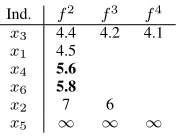
TABLE II

EXAMPLE OF THE INFORMATION AVAILABLE AT STAGE2OF THE ALGORITHM.T2_{= 5.6,AND ASSUME∆}2

c= 1.

Ind. f2 _f3 _f4 x3 4.4 4.2 4.1 x1 4.5

x4 5.6 x6 5.8

x2 7 6

x5 ∞ ∞ ∞

x4, x5, x6) have been evaluated on the lowest fidelity level (fit-nesses are in bold face to indicate they have just been evaluated at this fidelity level). The parent individuals(x1, x2, x3)have been evaluated at higher fidelity levels in previous generations. First, individuals are sorted according to f1_{. Based on f}1_, individuals x1, x3 and x6 would be accepted, the others discarded. The quality threshold isT1_=f1_{(x6) = 7. Now let} us assume that our logistic regression model predicts that with a fitness difference of more than∆1_c = 1.9, the probability for rank reversal is sufficiently low to be confident in the ranking. This means that solutions with f1 < T1−∆1c = 5.1 could

be safely accepted, and solutions with f1> T1+ ∆c = 8.9

could be safely discarded. In our case, this meansx1could be accepted, but since we already have higher fidelity evaluations, the solution is simply kept in the race. Solutionx5on the other hand is permanently discarded at this point, which is recorded as a fitness of∞on all higher fitness levels. Solutionsx6and x4 are re-evaluated on fidelity level 2, as they can be neither safely accepted nor safely discarded.

This then results in the information depicted in Table II. Note that the table is now sorted according to fidelity level 2, and x3 is the new best individual.T2 = 5.6 and assume ∆2

c = 1. In this case, x1 can be safely accepted (receiving fitness −∞ on higher fitness levels), whereas solutions x4 and x6 need to be evaluated on fidelity level 3, resulting in Table III. Finally, on fidelity level 3,T3_{= 5and with∆}3

c=0.4,

solutionsx2andx6can be safely discarded, whereasx4needs another evaluation at fidelity level 4. Then, the algorithm stops and simply picks the best solutions according to fidelity level 4 in the final summary Table IV, i.e., solutionsx1, x4, andx3.

C. Forcing

TABLE III

EXAMPLE OF THE INFORMATION AVAILABLE AT STAGE3OF THE ALGORITHM.T1_{= 5,AND ASSUME∆c= 0.4.}

Ind. f3 f4

x1 −∞ −∞

x3 4.2 4.1

x4 5

x2 6

x6 6.1

x5 ∞ ∞

TABLE IV

EXAMPLE OF THE FINAL INFORMATION AVAILABLE FOR THE SELECTION PROCESS.

Ind. f1 _f2 _f3 _f4

x1 5 4.5 −∞ −∞

x4 8 5.6 5 4.5

x3 6 4.4 4.2 4.1

x6 7 5.8 6.1 ∞

x2 9 7 6 ∞

x5 10 ∞ ∞ ∞

based on their low fidelity evaluation survive forever although they are actually quite poor with respect to the highest fidelity, we employ a method we call “forcing”: In each generation, from theµbest solutions and ignoring the fully evaluated ones, we pick the solution with the smallest estimated probability of reversal based on its highest fidelity level evaluated, and evaluate it to the highest fidelity level. This guarantees a minimal flow of highest fidelity information that can be used to update our probability models.

IV. NEW BENCHMARK PROBLEMS

In this section, we propose two new benchmark problems to test the performance of multi-fidelity optimization approaches. The first problem is a one-dimensional artificial test function designed to reflect some of the characteristics of multi-fidelity problems. The second problem is derived from a real engineer-ing application. To allow other researchers to compare with our results, the MATLAB code of the benchmark problems is publicly available [39].

A. Artificial Test Function

Intuitively, when thinking of multi-fidelity problems, we expect that the lower fidelity models provide a coarse approx-imation of the higher fidelity models, with less detail. Also, we expect that there may be vertical shifts (e.g., values from the low fidelity models are all higher than values from the high fidelity model) or lateral shifts of local optima (i.e., the position of a local optimum on lower fidelity models does not correspond to the position of the corresponding local optimum in the higher fidelity model). All these aspects have been engineered into our artificial test function. Since the function is one-dimensional, evaluation is quick and the function and the algorithm’s performance can be easily visualized, which makes it an ideal testbed during algorithm development.

There are 6 fidelity levels for the function, with fidelity 1 being the least accurate assumed to cost 1 unit of com-putational time, and fidelity 6 corresponding to the most

accurate estimate costing 6 units of computational time. The test function is visualized in Fig. 2. The mean squared error (MSE) and the Kendall Tau correlation coefficient of the various levels of fidelity relative to the highest fidelity level are listed in Table V. These metrics have been computed using 1000 uniformly spaced points. As expected, rank correlation increases with fidelity level, and MSE decreases with fidelity level.

-8 -6 -4 -2 0 2 4 6 8

Variable -20

-10 0 10 20 30 40 50

Function Value

Fidelity-1 Fidelity-2 Fidelity-3 Fidelity-4 Fidelity-5 Fidelity-6

Fig. 2. Test Function

TABLE V

MEAN SQUARED ERROR(MSE)AND THE RANK CORRELATION COEFFICIENT(KENDALLTAU)BETWEEN THE FIDELITIES OF THE

1-DIMENSIONAL ARTIFICIAL TEST FUNCTION.

MSE Kendall Tau

f1 _{35.3972 0.6380} f2 _{20.2299 0.6724} f3 _{9.9857 0.7853} f4 _{3.8126 0.8686} f5 _{0.8242 0.9409} f6 _{0.0000 1.0000}

The function can be extended to multiple dimensions by simply using the same function in each dimension, and adding up the values. For the two-dimensional version, the MSE and Kendall Tau values are reported in Table VI.

TABLE VI

MEAN SQUARED ERROR(MSE)AND THE RANK CORRELATION COEFFICIENT(KENDALLTAU)BETWEEN THE FIDELITIES OF THE

2-DIMENSIONAL ARTIFICIAL TEST FUNCTION.

MSE Kendall Tau

f1 _{78.8834 0.6694} f2 _{45.7713 0.7500} f3 _{22.9244 0.8292} f4 _{8.9905 0.8962} f5 _{1.9883 0.9528} f6 _{0.0000 1.0000}

B. Toysub Benchmark Problem

As a complement to the artificially designed

prob-Fig. 1. Artificial test function with 6 fidelity levelsf1−f6

f1 = min

(x−2)2,(x+ 2)2+ 2 (2)

f2 = min

(x−2)2+ 5 sinπ 2(x+ 1)

,(x+ 2)2+ 5 sinπ 2(x+ 1

+6

5

(3)

f3 = min

(x−2)2+ 5 sinπ 2(x+ 1)

+ 4 sin

π(x+3

2)

,(x+ 2)2+ 5 sinπ 2(x+ 1)

+ 4 sin

π(x+3

2) +2 5 (4)

f4 = min

(x−2)2_{+ 5 sin}π 2(x+ 1)

+ 4 sin

π(x+3

2)

+ 3 sin

2π(x+7 4)

, (5)

(x+ 2)2+ 5 sin π

2(x+ 1)

+ 4 sin

π(x+3 2)

+ 3 sin

2π(x+7

4) −2 5 (6)

f5 = min

(x−2)2+ 5 sin π

2(x+ 1)

+ 4 sin

π(x+3 2)

+ 3 sin

2π(x+7

4)

+ 2 sin

4π(x+15 8 )

, (7)

(x+ 2)2+ 5 sin _π

2(x+ 1)

+ 4 sin

π(x+3 2)

+ 3 sin

2π(x+7

4)

+ 2 sin

4π(x+15 8 ) −6 5 (8)

f6 = min

(x−2)2+ 5 sinπ 2(x+ 1)

+ 4 sin

π(x+3

2)

+ 3 sin

2π(x+7 4)

+ 2 sin

4π(x+15 8 )

+ sin (8π(x+ 2)), (9)

(x+ 2)2+ 5 sinπ 2(x+ 1)

+ 4 sin

π(x+3

2)

+ 3 sin

2π(x+7 4)

+ 2 sin

4π(x+15 8 )

+ sin (8π(x+ 2))−2

(10)

lem is designed to be more similar to a real-world problem. The task is to design a toy submarine (Fig. 3) with the goal to minimize the drag, while still obeying all volume constraints. The problem involves eight variables defining the geometry of the submarine as shown in Fig. 4. The design variables are: the position of the internal components along the Z-axis i.e. the position of the controller (ZC), position of the propeller

unit for pitch (ZV) and yaw (ZL) movements, position of the

battery compartment (ZB), smaller diameter (dt) and length

(lt) of the tail and shape variation coefficient (nn) and length

(ln) of the nose. The bounds of the variables are presented in

Equation 11. The drag is estimated using ANSYS FLUENT 13.0.

The overall problem can be formulated as follows:

Minimize:f(1) =D Variable bounds:

0≤ZC≤300 mm; 0≤ZV ≤300 mm

0≤ZB ≤300 mm; 0≤ZL≤300mm

35≤dt≤50 mm; 80≤lt≤150 mm

1.5≤nn≤3; 45≤ln≤100mm

(11)

However, testing each solution using the CFD solver would make solving the problem too time consuming to be a sensible benchmark. Also, only researchers with access to the ANSYS FLUENT 13.0 software would be able to replicate results or compare their algorithms. Since the body is axisymmetric, a quarter model of the bare hull can be used to reduce the CFD analysis costs, but it would still be too slow to be practical. To solve this predicament, we have generated 284 designs using Latin Hypercube Sampling and estimated their drag using ANSYS FLUENT 13.0. The velocity at the inlet was set to 0.5 m/s while that at the outlet was set to zero. We recorded the drag values for these designs after 5, 10, 25, 50, 75 and 100 iterations resulting in 6 different fidelity levels with computational cost of 5, 10, 25, 50, 75 and 100 units, respectively. This data was then “expanded” to the full range of the search space by learning six Gaussian

Process models based on the 284 design points, one for each fidelity level. These six Gaussian Process models hopefully correspond closely to the landscapes of the real CFD solver, but are much faster to evaluate and thus constitute a suitable benchmark problem.

The mean squared error and the correlation coefficient (Kendall Tau) between the various fidelity levels and the high-est fidelity level based on 1000 uniformly distributed random designs are presented in Table VIII. Again, Kendall Tau is increasing with increasing fidelity level, while mean squared error is generally decreasing (although not monotonically).

Fig. 3. USS Dallas RC toy submarine

TABLE VII

PERFORMANCE CRITERIA OF THEUSS DALLASRCTOY SUBMARINE

Vehicle particulars USS Dallas RC

Nose length 45 mm

Parallel middle body length 210 mm

Tail length 95 mm

Length overall 350 mm

Maximum diameter 60 mm

Length to diameter ratio 5.8 Wetted surface area 0.082385 m2 Displacement volume 0.000437 m3 Mass of the displaced water 437 g Total mass of the vehicle 430 g X-coordinate of CG -0.981462 mm Y-coordinate of CG -0.210313 mm Z-coordinate of CG 167.083 mm

X-coordinate of CB 0

Y-coordinate of CB 0

Z-coordinate of CB 163.375 mm

Nominal speed 0.5 m/s

Drag 0.0671897 N

TABLE VIII

MEAN SQUARED ERROR(MSE)AND THE RANK CORRELATION COEFFICIENT(KENDALLTAU)BETWEEN THE FUNCTIONS

MSE Kendall Tau

y1 _{0.0203 0.7735} y2 0.0011 0.8712

y3 0.0017 0.8936

y4 0.0000 0.9791

y5 0.0000 0.9899

y6 _{0.0000 1.0000}

V. EMPIRICALEVALUATION

A. Parameter Settings

As the underlying optimization algorithm, we uased a real coded evolutionary algorithm with simulated binary crossover and polynomial mutation [40]. The probability of crossover is set to 1 with a mutation probability of 0.1 for the simple test function and 0.125 for the Toysub problem. The distribution indices of crossover (ηc) and mutation(ηm) are set to 20

and30respectively, independent of the optimization problem. Population size is 20 for the simple one-dimensional function, and 48 for the more complicated Toysub problem. The total evaluation budget was limited to2000units for the simple test function and 100,000 units for the Toysub problem.

The initial probability threshold for MFEA is δ = 0.05 unless stated otherwise, and linearly decreased to zero over the course of the run to ensure that no selection errors are made at the late stages of the optimization run.

B. Performance Measure and Benchmarks

To evaluate the performance of our proposed MFEA al-gorithm, we compare it with the following alternative ap-proaches:

1) Fidelity-6:Evolutionary algorithm where every solution is evaluated with the highest fidelity model.

2) Fidelity-1:Evolutionary algorithm where every solution is evaluated with the lowest fidelity model.

3) Average: In principle, one could also compare with the performance using any other fixed fidelity model. However, for a real world problem, it would not be

clear which fidelity level would result in the best solution quality. To reflect this fact, we assume the user might pick a fidelity level at random. Then, the expected performance would just be the average of the expected performances of each fidelity level.

4) Progressive:Some people have suggested starting with a low fidelity model and then moving to a higher fidelity model over the course of the optimization. We have implemented this by dividing up the computational bud-get into equal parts, and using the same computational budget on each fidelity level.

We are interested in the highest fidelity performance of the solution returned by the algorithm. Independent of the algorithm variant, the final generation is evaluated to the highest fidelity to make sure that the best solution in the population is recognized and accounted for.

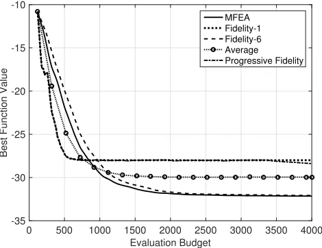
Different algorithms may have advantages at different stages of the run. For example, an algorithm using only the lowest fidelity can be expected to do well if the computational budget is very small, as it can still perform a few generations albeit with a crude fitness approximation. On the other hand, if the computational budget is very large, then we can assume that an algorithm only using the highest fidelity model will yield the best result. Thus it is important to look at the convergence plots of the algorithm. The convergence plots we use show the highest fidelity performance of the solution that would be returned at a particular point in time, where time includes the high fidelity evaluation of the final population.

The generation of the convergence plot is best explained by an example. Let us consider a run on the simple function with fixed fidelity 2. The initial population requires 40 cost units to evaluate at fidelity level 2. If we were to stop here, this population would be fully evaluated, which requires another 80 cost units (four additional fidelity levels for 20 solutions). So, our first entry on the convergence plot would be the best solution according to fidelity level 6, with a cost of 120 units. The algorithm continues from the level 2 evaluation, generates 20 children and selects the next population. On the convergence plot, we then plot the best solution based on fidelity level 6 with a cost of 160 units (40 for evaluating the initial population, 40 for evaluating the children, and 80 to bring all selected individuals to fidelity level 6, etc.).

All results reported are based on the average over 100 inde-pendent runs for the simple test function, and 30 indeinde-pendent runs for the Toysub problem.

C. Results on the Simple Test Function

The observations are reinforced also by looking at Ta-bles IX and X, which show the algorithm performance after a computational budget of 2000 units and as average over the runtime, respectively. While the Fidelity-6 approach yields the best performance at the end of the run, it is only marginally better than our MFEA and the difference is statistically not significant according to a Kolmogorov-Smirnov test with 5% significance level. In terms of average performance over the run, MFEA outperforms all other approaches in the table, although the difference to Fidelity-6 is again statistically not significant.

Similar observations hold for the 2D version of this test function, see Fig. 6.

0 500 1000 1500 2000

Evaluation Budget -17

-16 -15 -14 -13 -12 -11

Best Function Value

MFEA Fidelity-1 Fidelity-6 Average

Progressive Fidelity

Fig. 5. Convergence plot for various approaches on the simple 1D test function

0 500 1000 1500 2000 2500 3000 3500 4000 Evaluation Budget

-35 -30 -25 -20 -15 -10

Best Function Value

MFEA Fidelity-1 Fidelity-6 Average Progressive Fidelity

Fig. 6. Convergence plot for various approaches on the simple 2D test function

Fig. 7 examines the influence of the initial probability of reversal thresholdδ. As can be seen, the performance is quite robust to this parameter.

To gain a better understanding of the workings of the pro-posed algorithm, we investigated various other aspects on the 1D artificial test function. Fig. 8 shows the misclassification percentage over time, i.e., the percentage of solutions that

TABLE IX

PERFORMANCE OBTAINED AT END OF RUN FOR SIMPLE TEST FUNCTION.

Test function Best Mean Median Worst Std Err MFEA -16.475 -16.259 -16.469 -14.462 0.057 Fidelity-1 -14.071 -14.002 -14.000 -13.965 0.002 Fidelity-2 -14.346 -13.997 -14.000 -13.609 0.008 Fidelity-3 -16.398 -14.150 -14.005 -13.577 0.054 Fidelity-4 -16.371 -15.851 -16.001 -13.933 0.060 Fidelity-5 -16.475 -15.786 -16.000 -13.534 0.067 Fidelity-6 -16.475 -16.286 -16.469 -14.375 0.055 Progr. Fidelity -14.475 -14.194 -14.213 -13.679 0.021

TABLE X

AVERAGE PERFORMANCE OVER THE RUN ON THE SIMPLE TEST FUNCTION.

Test function Best Mean Median Worst Std Err MFEA -16.475 -15.592 -15.731 -13.027 0.070 Fidelity-1 -14.149 -13.922 -13.973 -13.434 0.016 Fidelity-2 -14.557 -13.962 -14.024 -12.891 0.029 Fidelity-3 -16.035 -14.254 -14.217 -12.989 0.055 Fidelity-4 -16.348 -15.490 -15.667 -13.549 0.064 Fidelity-5 -16.398 -15.355 -15.522 -13.487 0.073 Fidelity-6 -16.475 -15.402 -15.650 -10.308 0.094 Progr. Fidelity -14.339 -13.971 -14.024 -13.208 0.020

0 500 1000 1500 2000

Evaluation Budget

-17 -16 -15 -14 -13 -12 -11

Best Function Value

MFEA-0.02 MFEA-0.05 MFEA-0.10

Fig. 7. Convergence plot for various probability of reversal thresholdsδon the simple test function

have been unjustly (according to highest fidelity level) carried forward from one generation to the next. If this is zero, then we know survival selection works perfectly as if all individuals would have been evaluated at the highest fidelity level. As can be seen, for this simple test problem there is a small misclassification percentage at the beginning of the run, at least for δ= 0.05 andδ= 0.1. It then quickly goes to zero, and there are no more errors in selection for the remainder of the run.

0 500 1000 1500 2000 Evaluation Budget

0 0.5 1 1.5 2 2.5 3 3.5 4 4.5 5

Misclassification Percentage

MFEA-0.02 MFEA-0.05 MFEA-0.10

Fig. 8. Percentage of misclassified individuals over the run, for different levels of reversal thresholdδ

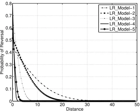
the algorithm zooms into a region around the optimum, and in this local region the correlation between the models is higher than over the entire search space.

0 10 20 30 40 50

0 0.1 0.2 0.3 0.4 0.5 0.6 0.7 0.8

Distance

Probability of Reversal

LR_Model−1 LR_Model−2 LR_Model−3 LR_Model−4 LR_Model−5

Fig. 9. Learned model of probability of reversal just after initial population has been generated, for fidelity levels 1-5.

In our tests so far, we have assumed there are six levels of fidelity. However, a simulation run may be interrupted at many more possible stopping points, and each could be regarded as a fidelity level. There is a fundamental trade-off: More fidelity levels should allow our method to make better choices (albeit with diminishing returns, i.e., the difference between using 2 and 4 fidelity levels may be significant, whereas the difference between using 102 and 104 fidelity levels is probably marginal), but increases the training effort as we need to learn and update the probability of reversal for every fidelity level. To better understand the impact of the number of fidelity levels, Fig. 11 compares the convergence of MFEA that has access to all six fidelity levels with an MFEA that is only allowed to use fidelity levels 1 and 6. As expected, the larger number of fidelity levels leads to a slightly faster convergence.

0 10 20 30 40 50 60

0 0.1 0.2 0.3 0.4 0.5 0.6 0.7 0.8 0.9

Distance

Probability of Reversal

LR_Model−1 LR_Model−2 LR_Model−3 LR_Model−4 LR_Model−5

Fig. 10. Learned model of probability of reversal at the end of an optimization run, for fidelity levels 1-5.

0 500 1000 1500 2000

Evaluation Budget -17

-16 -15 -14 -13 -12 -11

Best Function Value

MFEA (6 Fidelity Levels) MFEA (2 Fidelity Levels)

Fig. 11. Comparison of convergence with different number of fidelity levels in forced condition for simple test function

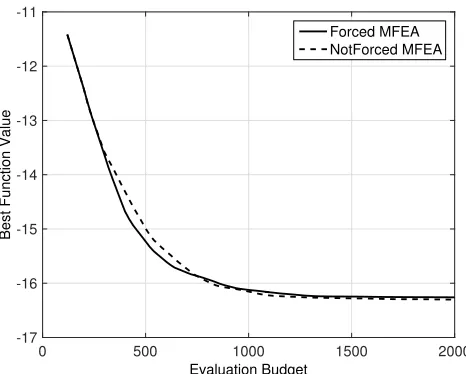
Finally, we wanted to understand the benefit of forcing at least one individual to be evaluated at the highest fidelity level in each generation. As Fig. 12 shows, in this example the effect of forcing on convergence seems marginal, with perhaps a small advantage in the early phases of the run.

D. Results on the Toysub Problem

0 500 1000 1500 2000 Evaluation Budget

-17 -16 -15 -14 -13 -12 -11

Best Function Value

Forced MFEA NotForced MFEA

Fig. 12. Convergence plot for MFEA with and without forcing on the simple test function

allow Fidelity-6 to converge. Our MFEA converges relatively quickly, and finds a very good solution within the given com-putational budget. In particular, MFEA only required about 40,000 computational units to reach the same solution quality that the high fidelity approach (Fidelity-6) has reached after a computational budget of 100,000 units, thus effectively saving 60% of the computational cost.

0 2 4 6 8 10

Evaluation Budget _×104 0.06

0.07 0.08 0.09 0.1 0.11 0.12

Best Function Value

MFEA Fidelity-1 Fidelity-6 Average Progressive Fidelity

Fig. 13. Convergence plot for various probability of reversal thresholds on the Toysub test problem.

Looking at the results in Tables XI and XII, this general impression is confirmed. MFEA significantly outperforms the progressive fidelity approach also Fidelity 1, 2 and 6. Fidelity-4 reaches a slightly better mean performance at the end than MFEA, however the difference is not statistically significant. In terms of average performance over the run, Fidelity-3 is slightly better, but again not statistically significant. Note that in a real world problem, one would not know which fidelity would yield best results with a given computational budget, so comparing the MFEA to the best of the single fidelity models is not a fair comparison.

Again, to gain a deeper understanding of the algorithm, we examine some additional aspects. When looking at the benefit of forcing (Figure 14), this time there is a clearly visible benefit.

0 2 4 6 8 10

Evaluation Budget _×104 0.06

0.07 0.08 0.09 0.1 0.11 0.12

Best Function Value

Forced MFEA NotForced MFEA

Fig. 14. Convergence plot for MFEA with and without forcing on the Toysub test problem

TABLE XI

BEST FUNCTION VALUE: TOYSUB

Toysub Best Mean Median Worst Std Err MFEA 0.047 0.067 0.066 0.093 0.002 Fidelity-1 0.052 0.086 0.087 0.102 0.002 Fidelity-2 0.056 0.077 0.077 0.102 0.002 Fidelity-3 0.056 0.070 0.064 0.099 0.003 Fidelity-4 0.048 0.065 0.063 0.081 0.001 Fidelity-5 0.058 0.070 0.069 0.088 0.002 Fidelity-6 0.062 0.074 0.071 0.093 0.002 Progr. Fidelity 0.052 0.085 0.086 0.102 0.002

TABLE XII

AVERAGE PERFORMANCE OVER THE RUN ON THETOYSUB PROBLEM

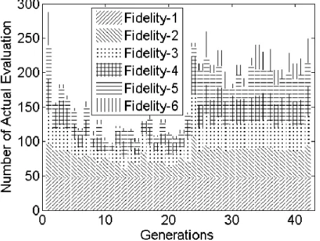
Toysub Best Mean Median Worst Std Err MFEA 0.056 0.078 0.078 0.097 0.002 Fidelity-1 0.055 0.086 0.087 0.103 0.002 Fidelity-2 0.059 0.079 0.079 0.103 0.002 Fidelity-3 0.063 0.076 0.072 0.102 0.002 Fidelity-4 0.068 0.080 0.079 0.091 0.001 Fidelity-5 0.071 0.088 0.088 0.100 0.001 Fidelity-6 0.076 0.092 0.093 0.106 0.002 Progr. Fidelity 0.055 0.086 0.087 0.103 0.002

makes a selection based on lower fidelity levels less reliable, and also because we use a linearly decreasing threshold for the probability of reversal.

Fig. 15. Number of fitness evaluations performed at different fidelity levels, over the course of the run

Finally, we once again compare the convergence of MFEA that uses 6 fidelity levels to one that uses only fidelity levels 1 and 6. As can be seen in Fig. 16, the larger number of fidelity levels is again beneficial, and the difference appears larger than for the artificial test problem in Fig. 11.

0 2 4 6 8 10

Evaluation Budget _×104

0.06 0.07 0.08 0.09 0.1 0.11 0.12

Best Function Value

MFEA (6 Fidelity Levels) MFEA (2 Fidelity Levels)

Fig. 16. Comparison of convergence with different number of fidelity levels in forced condition for Toysub test problem

E. Additional Test Problems

To better understand in what situations our algorithm might work well and whether it is able to adapt to different situations, we designed two additional test problems. In the first one, PF1, all the fidelities are identical and correspond to fidelity level 6 of our simple artificial test function. In such a case, clearly only using fidelity 1 is the best possible strategy, as higher fidelity levels do not provide more accurate information but

only incur a higher computational cost. The opposite scenario is a problem where the different fidelities have nothing in common. We designed such a function PF2 by assigning each fidelity level independently a different function, sometimes shifted to make sure they do not happen to have the same optimum, see Table XIII and Table XIV for the MSE and Kendall Tau correlation. For such a function, the best strategy should be to only use fidelity level 6, as lower fidelity levels do not provide useful information.

TABLE XIII

DIFFERENT FIDELITIES OF FUNCTIONPF2. THE VARIABLE(X)RANGE FOR ALL LEVELS IS SET TO[-8, 8].

Fidelity Function f1(x) Ackley(x-0.8) f2(x) Griewank(x-0.6) f3(x) Sphere(x) f4(x) -1×Rastrigin(x-0.1) f5(x) Zakharov(x-0.4) f6(x) -1×Levy(x-0.2)

The results on these two problems are depicted in Fig. 17 and 18. As expected, for PF1, using fidelity 1 only would perform best. Our MFEA is a bit slower in the beginning as it has to learn first that higher fidelity levels are not helpful, and the forcing mechanism forces the algorithm to fully evaluate at least one individual in every generation. Still, it is much faster than picking a fidelity level at random or using the highest fidelity only. For example, where the algorithm using fidelity 6 requires approx. 1500 function evaluations to converge, MFEA only requires a third, i.e., approx. 500 function evaluations. Using a progressive fidelity level also works very well for this function, basically because it starts with fidelity 1 and has almost converged by the time it switches to the next higher fidelity level.

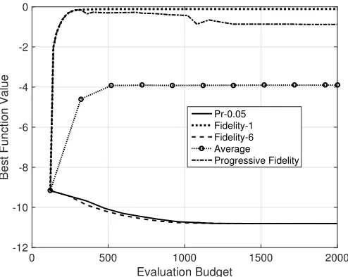
For PF2, clearly fidelity level 6 is required to allow any sensible optimization. Again, MFEA adapts to that scenario and performs almost as well as the algorithm with pre-set fidelity level 6. MFEA learns the correct fidelity level very quickly and, different from PF1, forcing is not causing unnecessary function evaluations. The algorithms with a pre-set lower fidelity level optimize the wrong function, and their performance actually deteriorates compared with the random initial population.

From these experiments, we conclude that MFEA is very effective at learning the right fidelity level and thus should work well in a wide range of problem types.

TABLE XIV

MEAN SQUARED ERROR(MSE)AND THE RANK CORRELATION COEFFICIENT(KENDALLTAU)BETWEEN THE FUNCTIONS INPF2.

MSE Kendall Tau

f1 _{0.2441E+03 -0.7124} f2 _{0.0177E+03 0.1047} f3 _{1.0159E+03 -0.6226} f4 _{0.6857E+03 0.6402} f5 16.2488E+03 -0.7035

0 500 1000 1500 2000 Evaluation Budget

-17 -16 -15 -14 -13 -12 -11

Best Function Value

MFEA Fidelity-1 Fidelity-6 Average Progressive Fidelity

Fig. 17. Convergence plot for various approaches on the PF1 test function.

0 500 1000 1500 2000

Evaluation Budget

-12 -10 -8 -6 -4 -2 0

Best Function Value

Pr-0.05 Fidelity-1 Fidelity-6 Average

Progressive Fidelity

Fig. 18. Convergence plot for various approaches on the PF2 test function.

VI. CONCLUSION

In this paper, a novel learning based approach is introduced for the solution of optimization problems involving expensive simulation models that can be stopped early to obtain a computationally less expensive low fidelity model. Multiple logistic regression models are learned and used to rank and identify individuals in the population that can be confidently included in the next population or discarded based on partially converged simulation results. The behavior of the scheme is illustrated on two new benchmark problems: a simple artificial test function as well as a close-to-real-world higher dimensional mechanical design problem. The performance of the algorithm is compared with different single fidelity optimization strategies and a progressive fidelity strategy, and the results show that our proposed MFEA is able to produce good results independent of the available computational budget and without requiring to specify a fidelity level. It significantly outperforms alternative approaches using progressive fidelity levels or choosing the fidelity level at random.

Several extensions to the current approach seem interesting.

• In the current form, the logistic regression models are

built using all available data, but it would be possible to build local models instead of global models. In such a case, for every point under consideration, a number of neighboring points needs to be identified which would then be used to build the logistic regression models, better reflecting the local characteristics of the search space.

• The approach should be extended to handle also con-straint problems, and even problems where the objectives and constraints may not all have the same number of fidelity levels.

• The approach may be extended to multi-objective

opti-mization problems. An extension along these lines would then pave the way for an easier adoption within the multidisciplinary design optimization (MDO) community.

ACKNOWLEDGMENTS

The last author would like to acknowledge support from the Australian Research Council (ARC) Future Fellowship. Visitors grant from the School of Engineering and Information Technology (SEIT) and UNSW Canberra is also gratefully acknowledged.

REFERENCES

[1] Y.-J. Gong, W.-N. Chen, Z.-H. Zhan, J. Zhang andY. Li, Q. Zhang, and J.-J. Li. Distributed evolutionary algorithms and their models: A survey of the state-of-the-art. Applied Soft Computing, 34:286–300, 2015. [2] M. Bhattacharya. Evolutionary approaches to expensive optimisation.

International Journal of Advanced Research in Artificial Intelligence, 2(3):53–59, 2013.

[3] Y. Jin and J. Branke. Evolutionary optimization in uncertain environments-a survey. Evolutionary Computation, IEEE Transactions on, 9(3):303–317, 2005.

[4] Y. Jin. A comprehensive survey of fitness approximation in evolutionary computation.Soft Computing - A Fusion of Foundations, Methodologies and Applications, 9:3–12, 2005.

[5] Y. Jin. Surrogate-assisted evolutionary computation: Recent advances and future challenges. Swarm and Evolutionary Computation, 1(2):61– 70, 2011.

[6] L. Shi and K. Rasheed. A survey of fitness approximation methods applied in evolutionary algorithms. In Yoel Tenne and Chi-Keong Goh, editors, Computational Intelligence in Expensive Optimization Problems, volume 2 ofAdaptation, Learning, and Optimization, pages 3–28. Springer Berlin Heidelberg, 2010.

[7] M. A. El-Beltagy and A. J. Keane. Evolutionary optimization for compu-tationally expensive problems using gaussian processes. InInternational Conference on Artificial Intelligence, pages 708–714. CSREA Press, 2001.

[8] M. Emmerich, A. Giotis, M. ¨Ozdemir, T. B¨ack, and K. Giannakoglou. Metamodel-assisted evolution strategies. InInternational Conference on Parallel Problem Solving from Nature, LNCS, pages 361–370, London, UK, UK, 2002. Springer-Verlag.

[9] D. Lim, Yaochu Jin, Yew-Soon Ong, and B. Sendhoff. Generalizing surrogate-assisted evolutionary computation.Evolutionary Computation, IEEE Transactions on, 14(3):329–355, june 2010.

[10] D. Eby, R. C. Averill, W. F. Punch III, and E. D. Goodman. Evaluation of injection island GA performance on flywheel design optimization. In I. C. Parmee, editor,Adaptive Computing in Design and Manufacture, pages 121–136. Springer, 1998.

[11] K. Sastry, D. E. Goldberg, and M. Pelikan. Don’t evaluate, inherit. InGenetic and Evolutionary Computation Conference, pages 551–558. Morgan Kaufmann, 2001.

[12] J. Branke and C. Schmidt. Fast convergence by means of fitness estimation. Soft Computing Journal, 9:13–20, 2005.

[14] B. Liu, Q. Zhang, and G. Gielen. A gaussian process surrogate model assisted evolutionary algorithm for medium scale expensive optimization problems.IEEE Transactions on Evolutionary Computation, 18(2):180– 192, 2014.

[15] T. Hildebrandt and J. Branke. On using surrogates with genetic programming.Evolutionary Computation, 23(3):343–367, 2015. [16] L. Gr¨aning, Y. Jin, and B. Sendhoff. Individual-based management of

meta-models for evolutionary optimization with application to three-dimensional blade optimization. In Y.-S. Ong and Y. Jin, editors,

Evolutionary Computation in Dynamic and Uncertain Environments. Springer, 2007.

[17] Y.-S. Ong, P. B. Nair, and A. J. Keane. Evolutionary optimization of computationally expensive problems via surrogate modeling. AIAA Journal, 41(4):687–696, 2003.

[18] Z. Zhou, Y.-S. Ong, M.-H. Lim, and B.-S. Lee. Memetic algorithm using multi-surrogates for computationally expensive optimization problems.

Soft Computing, 11(10):957–971, 2007.

[19] Z. Zhou, Y.-S. Ong, P. B. Nair, A. J. Keane, and K. Y. Lum. Combining global and local surrogate models to accelerate evolutionary optimiza-tion. IEEE Transactions on Systems, Man, and Cybernetics, Part C: Applications and Reviews, 37(1):66–76, 2007.

[20] Y. Chen, W. Xie, and X. Zou. How can surrogates influence the convergence of evolutionary algorithms? Swarm and Evolutionary Computation, 12:18–23, 2013.

[21] H. Ulmer, F. Streichert, and A. Zell. Evolution strategies with controlled model assistance. InCongress on Evolutionary Computation, pages 1569–1576. IEEE, 2004.

[22] T. P. Runarsson. Constrained evolutionary optimization by approximate ranking and surrogate models. InParallel Problem Solving from Nature, number 3242 in LNCS, pages 401–410. Springer, 2004.

[23] J. Ziegler and W. Banzhaf. Decreasing the number of evaluations in evolutionary algorithms by using a meta-model of the fitness function. InEuroGP, volume 2610 ofLNCS, pages 264–275. Springer, 2003. [24] T. Takahama and S. Sakai. Reducing function evaluations in differential

evolution using rough approximation-based comparison. InCongress on Evolutionary Computation, pages 2307–2314. IEEE, 2008.

[25] T. Takahama and S. Sakai. Reducing function evaluations using adaptively controlled differential evolution with rough approximation model. In Y. Tenne and C.-K. Goh, editors,Computational Intelligence in Expensive Optimization Problems, pages 111–129. Springer, 2010. [26] M. N. Le, Y. S. Ong, S. Menzel, Y. Jin, and B. Sendhoff. Evolution by

adapting surrogates. Evolutionary Computation, 21(2):313–340, 2013. [27] Y. Tenne. An optimization algorithm employing multiple metamodels

and optimizers. International Journal of Automation and Computing, 10(3):227–241, June 2013.

[28] T. Ray, H. Tsai, and C. Tan. Effects of solver fidelity on a parallel search algorithm’s performance for airfoil shape optimization problems. InAIAA/ISSMO Symposium on Multidisciplinary Analysis and Optimiza-tion, 2002.

[29] M. Sefrioui and J. Periaux. A hierarchical genetic algorithm using multiple models for optimization. InParallel Problem Solving from Nature, number 1917 in LNCS, pages 879–888. Springer, 2000. [30] I. C. Kampolis and K. C. Giannakoglou. A multilevel approach to

single- and multiobjective aerodynamic optimization.Computer methods in applied mechanics and engineering, 197:2963–2975, 2008. [31] M. A. El-Beltagy and A. J. Keane. A comparison of various

optimiza-tion algorithms on a mulilevel problem. Engineering Applications of Artificial Intelligence, 12:639–654, 1999.

[32] D. Lim, Y. S. Ong, Y. Jin, and B. Sendhoff. Evolutionary optimization with dynamic fidelity computational models. In De-Shuang Huang, Donald C. Wunsch, Daniel S. Levine, and Kang-Hyun Jo, editors, Ad-vanced Intelligent Computing Theories and Applications. With Aspects of Artificial Intelligence, volume 5227 ofLNCS, pages 235–242. Springer Berlin Heidelberg, 2008.

[33] J. Branke, T. Hildebrandt, and B. Scholz-Reiter. Hyper-heuristic evolution of dispatching rules: A comparison of rule representations.

Evolutionary Computation, 23(2):249–277, 2015.

[34] A. I. J. Forrester, N. W. Bressloff, and A. J. Keane. Response surface model evolution. InAIAA Computational Fluid Dynamics Conference, 2003.

[35] A. I. J. Forrester, N. W. Bressloff, and A. J. Keane. Optimization using surrogate models and partially converged computational fluid dynamics simulations.Proceedings of the Royal Society A, 462:2177–2204, 2006. [36] L. Le Gratiet and C. Cannamela. Cokriging-based sequential design strategies using fast cross-validation techniques for multi-fidelity com-puter codes.Technometrics, 57(3):418–427, 2015.

[37] Y. Cao, Y. Jin, M. Kowalczykiewicz, and B. Sendhoff. Prediction of convergence dynamics of design performance using differential recurrent neural networks. InInternational Joint Conference on Neural Networks, pages 529–534. IEEE, 2008.

[38] C. Schmidt, J. Branke, and Steve Chick. Integrating techniques from statistical ranking into evolutionary algorithms. In Applications of Evolutionary Computation, number 3907 in LNCS, pages 753–762. Springer, 2006.

[39] Multi-fidelity benchmark matlab code. http://www.mdolab.net/Ray/Research-Data/MFGAProblems.zip. [40] K. Deb. Multi-objective optimization using evolutionary algorithms.

Wiley, 2001.

Juergen Branke is Professor of Operational Re-search and Systems at Warwick Business School, University of Warwick, UK. He received his PhD from the University of Karlsruhe, Germany, in 2000 and has been an active researcher in the area of natuinspired optimization since 1994. His re-search interests include multiobjective optimization, handling of uncertainty in optimization, dynamically changing optimization problems, and the design of complex systems.

Md Asafuddoula received the B.Sc. degree in Computer Science and Engineering from Chittagong University of Engineering and Technology at Chit-tagong, Bangladesh, in 2008 and the Ph.D. degree in Computer Science in University of New South Wales at Canberra, Australia, in 2014. He is currently a Re-search Associate with the School of Engineering and Information Technology, University of New South Wales at Canberra, Australia. His current research interests include evolutionary optimization, machine learning, constraint handling, many-objective opti-mization, robust design optimization and multi-fidelity based optimization.

Kalyan S. Bhattacharjeereceived the B.Tech and M.Tech degree in Ocean Engineering and Naval Ar-chitecture from Indian Institute of Technology (IIT), Kharagpur, in 2012 and 2013 respectively. He is currently a Postgraduate Researcher with the School of Engineering and Information Technology, Uni-versity of New South Wales at Canberra, Australia. His primary focus of research lies on handling com-putationally expensive optimization which includes surrogate assisted optimization, multi-fidelity based optimization and multi/many-objective optimization