Approximate Bayesian computation for infectious disease modelling

Contents lists available atScienceDirect

Epidemics

journal homepage:www.elsevier.com/locate/epidemics

Approximate Bayesian Computation for infectious disease modelling

Amanda Minter

, Renata Retkute

a_{Centre for the Mathematical Modelling of Infectious Diseases, London School of Hygiene and Tropical Medicine, London, UK} b_{The Zeeman Institute for Systems Biology and Infectious Disease Epidemiology Research, University of Warwick, UK}

A R T I C L E I N F O Keywords:

Approximate Bayesian Computation R

Epidemic model Stochastic model Spatial model

A B S T R A C T

Approximate Bayesian Computation (ABC) techniques are a suite of modelfitting methods which can be im-plemented without a using likelihood function. In order to use ABC in a time-efficient manner users must make several design decisions including how to code the ABC algorithm and the type of ABC algorithm to use. Furthermore, ABC relies on a number of user defined choices which can greatly effect the accuracy of estimation. Having a clear understanding of these factors in reducing computation time and improving accuracy allows users to make more informed decisions when planning analyses. In this paper, we present an introduction to ABC with a focus of application to infectious disease models. We present a tutorial on coding practice for ABC in R and three case studies to illustrate the application of ABC to infectious disease models.

1. Introduction

Mathematical models can be used to predict infectious disease dy-namics at multiple scales. Modelfitting, the process of estimating the parameters of the mathematical model from data, can be performed using a number of different methods. For infectious disease models, researchers are often confronted with missing data due to the nature of partially observed epidemics. Methods are needed tofit these models to data in an accurate and time efficient manner. In the Bayesian frame-work model parameters are assumed to be random variables and therefore have probability distributions, we seek to estimate the pos-terior distribution of these parameters (Gelman et al., 2013).

Approximate Bayesian Computation (ABC) methods can be used to approximate these posterior distributions when a likelihood function is intractable or not known (Beaumont et al., 2002), and can be used when the data available are coarse or complex. The ABC rejection al-gorithmPerez-Lezaun et al. (1999)is the most straight-forward of ABC methods yet ABC methods often yield inefficient sampling of the parameter space (Sadegh and Vrugt, 2014). As such, other algorithms with more efficient sampling schemes have been developed. The ABC-Sequential Monte Carlo (ABC-SMC) algorithm, provides a computa-tionally efficient estimation procedure compared to traditional ABC rejection algorithms (Toni et al., 2009).

ABC is a powerful tool for modelfitting and has a lot offlexibility with its application. However, this also means that the user must be

able to defend, and is responsible for all of these choices. There is an existing body of literature on ABC tutorials. In particular, for an starting introduction to ABC in generalSunnåker et al. (2013), for further ABC examples, including model selection seeToni et al. (2009), for tutorial on ABC for stochastic epidemic modelsKypraios et al. (2017),Hartig et al. (2002),McKinley et al. (2018), for comparison of likelihood-based Markov Chain Monte Carlo and ABC in epidemic modellingMcKinley et al. (2009), for examples for population genetics seeMarjoram et al. (2003),Beaumont et al. (2002).

The purpose of this paper is to provide a tutorial on ABC for in-fectious disease models for readers with very little experience in model

fitting. To that end, we provide a gentle introduction to the concept from the Bayesian inference paradigm followed by a presentation of how the ABC algorithm can be implemented in R. We present the im-plementation of ABC using three case studies to highlight the different approaches that can be taken to perform modelfitting using ABC. Case study 1 is an introductory example which illustrates the application of the ABC-rejection algorithm to a deterministic epidemic model, with a particular focus on the power of ABC based on the model to befitted and the data available.

Case study 2 is a stochastic compartmental model with age-struc-ture, i.e. the model where population is divided into compartments classified by the infection status and age of the host (Anderson and May, 1991). The dynamics of many childhood infections such as measles (Babad et al., 1995), whooping cough (Campbell et al., 2015),

https://doi.org/10.1016/j.epidem.2019.100368

Received 22 February 2019; Received in revised form 20 August 2019; Accepted 30 August 2019

Abbreviations:ABC, Approximate Bayesian Computation; SMC, Sequential Monte Carlo; NN, nearest neighbour ⁎_{Corresponding author.}

E-mail address:[email protected](A. Minter). 1_{These authors contributed equally to this work..}

1755-4365/ © 2019 Published by Elsevier B.V. This is an open access article under the CC BY-NC-ND license (http://creativecommons.org/licenses/BY-NC-ND/4.0/).

chickenpox (Schuette, 1999) and rubella (Kanaan and Farrington, 2005) can be described by age-structured compartmental model. In this case study we will investigate the 2010 measles outbreak in Malawi (Minetti et al., 2013) with the data consisting of weekly cases and percentage of cases in three age groups. Case study 3 uses an individual-based model which accounts for the spatial interaction between in-dividual hosts (Keeling and Rohani, 2007). These models have been used to investigating the spatial dynamics of foot-and-mouth disease (Keeling et al., 2001), avian influenza (Hill et al., 2017) or transmission of visceral leishmaniasis (Chapman et al., 2018). In this case study we will investigate citrus tristeza virus spread in an orchard (Marcus et al., 1984) with data consisting of maps of disease incidence observed at discrete times.

2. Approximate Bayesian Computation

The paradigm of Bayesian inference is based on the idea of updating belief with new evidence (Gelman et al., 2013). If we denoteθour mathematical model parameters andDour data, then we can use Bayes rule to determine the posterior distribution of the parameters given the data,P(θ|D):

=

P θ D P D θ P θ

P D ( | ) ( | ) ( )

( ) (1)

∝P D θ P θ( | ) ( ) (2)

whereP(θ) is the prior distribution (which represents our prior belief) andP(D|θ) is the likelihood function, the probability density function for the data given the parameters. The second equation is written without the marginal likelihood of the data,P(D), as the value ofP(D) does not depend onθ. Hence we can say thatP(θ|D) is proportional to the numerator of Eq. (1).

ABC is a method for approximating the posterior probabilityP(θ|D) without a using likelihood function (Beaumont, 2010). To illustrate this, we willfirst present a basic ABC algorithm, the ABC rejection al-gorithm (Perez-Lezaun et al., 1999; Toni et al., 2009). The algorithm ‘accepts’ proposed parameter values, so called particles, based on whether the distanced() between the dataDand the model simulated dataD*is less than or equal to some thresholdϵ. The steps of the ABC-rejection algorithm are as follows:

1. Sampleθ*from the prior distributionP(θ).

2. Simulate data set from the model, using parametersθ*_{, to getD*.} 3. Ifd(D,D*_{)≤ϵacceptθ* otherwise reject.}

4. Repeat untilNparticles (the parameter values or parameter sets)θ* ={ *;θi i=1, …, }n are accepted.

whered(D,D*_{) is some distance measure between the model output} and the data, andϵis a tolerance value which is chosen by the user. The N accepted samples provide an approximation of the posterior dis-tribution of the model parametersθ,

≈ ≤

P θ D( | ) P θ d D D( | ( , *) ϵ) (3).

The distance measure d(D, D*_{) implies it is possible to directly} compare the model output to the data. For example, if the data are daily cases of an infection and we wish to estimate parameters of a Susceptible-Infected-Recovered model (SIR), the user could compare the sum of the squared differences between the number of infected individuals between the data and that which is predicted by the model over time i.e. d D D( , *)= ∑T_t=1(Dt−Dt*)2 where time is denoted by t= 0,…,T.

When working with infection dynamics, there is often missing data or the data may consist of one measure of an epidemic. For example, say the data consists of thefinal size of the epidemic which we denoteμ. Then we simulate from the underlying model to calculate thefinal size μ*

from our simulated data setD*using a‘summary statistic’S(D*). In

this example the‘summary’is the calculation of the final size of the epidemic but it can take a form of other aggregated measures such as the number of infected individuals in different age groups, or the number of infected individuals in particular geographical locations. Then step 3 in the ABC-rejection algorithm becomes,

1. Ifd(μ,μ*_{)≤ϵ, whereμ* =S(D*), acceptθotherwise reject.} An intersection metric can be used when there is more then one summary statistic (McKinley et al., 2018):

∏

= ≤

P D Dˆ ( | *) (d ( ,D D*) ϵ ),

m

m m

(4) whereis a binary operator andmis a number of summary statistics. The intersection metrics ensures that model run is accepted only if all criteria are satisfied, but requires the specification of multiple tolerance values at each generation.

2.1. Implementing ABC in R

In this section we illustrate how to implement an efficient ABC-re-jection algorithm in R. To implement ABC in R, there are a number of techniques that can be used for fast computation. We direct the readers toVisser et al. (2015), Wilson et al. (2014)for tutorials on efficient coding. For ABC-rejection algorithms, computation time can be de-creased by pre-allocation of memory to store the accepted particles, memorization (do not repeat calculations with the loop) of data cal-culations, not printing unnecessarily, and vectorisation where possible in the function calls.

Fig. 1shows the code for the ABC-rejection algorithm implemented in R. There are two distinct sections to the code: the initial set up which occurs outside of the while loop (the initialisation), and the ABC-re-jection algorithm which occurs in the while loop. The initialisation requires the user to specify inputs related to the ABC-rejection algo-rithm. Specifically, the desired number of particles (N) and the toler-ance value (ϵ). The user then needs to pre-allocate memory to store the results of the ABC-rejection algorithm. For a model with one parameter this would be a vector, if the model had multiple parameters then this would be a matrix. In addition, the user may wish to store the distances which were accepted, which would require an additional column in the matrix.

The ABC-rejection algorithm is performed in a while loop with a counter (i) initiated outside of the loop. Within the while loop, we utilise existing R functions to propose values from the prior distribu-tions (for examplerunif,rnorm). Then we recommend user coded functions to separate the ABC-rejection steps. Data are simulated using the epidemic model and with the proposed parameters (θ*

) using the user coded functionrun_model. The distance between the data and the model output is calculated using the user coded function calc_-distance. If the distance is less than or equal to the tolerance, ep-silon, the current parameter value is stored and the counter is up-dated. Additionally, if a summary statistic is to be used the user can code a function to calculate the statistic using the simulated data set. The loop continues until the desired number of accepted particles (N) have been found. The user could specify a tolerance value that is too small for any proposed value to be accepted which could result in an infinite while loops. To avoid this the user could define a maximum number of iterations to be executed.

so-called embarrassingly parallel. Ultimately, the ABC-rejection algo-rithm is slow due to its inefficient proposal of parameter values. In the next section, we introduce an extension to the ABC-rejection algorithm which uses a more efficient scheme to sample the parameter space. 2.2. Speeding up ABC using alternative algorithms: ABC-SMC

Sequential Monte Carlo (ABC-SMC) is an ABC approach where a sequence of distributions is constructed by gradually decreasing toler-anceϵ. The ABC-SMC algorithm starts by sampling afinite number of parameter sets (particles) from the prior distribution and each inter-mediate distribution (called a generation) is obtained as a weighted sample from the previous distribution that has been perturbed through a kernelK(θ|θ*_).

Pseudocode for an ABC-SMC algorithm are as follows (Toni et al., 2009; McKinley et al., 2018):

1. Set the number of generationsG, and the number of particlesN. 2. Set the tolerance scheduleϵ1<ϵ2<⋯, <ϵG. Set the generation

indicatorg= 1.

3. Set particle indicatori= 1.

4. If g= 1, sample θ** _{from the prior distributionP(θ). If g> 1,} sampleθ*_{from the previous generation {θ}

g−1} with weights{wg−1},

and perturb the particle to obtainθ**∼K(θ|θ*). 5. IfP(θ**_{) = 0, return to step 4.}

6. Generate ndata setsD**_j from the model usingθ**_{and calculate}

= ∑₌ ≤

P D Dˆ ( | **) (1/ )n n_{j 1} ( ( ,d D D**)j ϵ )g.

7. IfP D Dˆ ( | **)=0, return to step 4.

8. Setθ_g( )i =θ**_{and calculated corresponding weight of the accepted} particlei

= ⎧

⎨ ⎪

⎩ ⎪

=

∑₌ − − >

w

P D D P θ g

P D D P θ

w K θ θ g

ˆ ( | **) ( **), if 1. ˆ ( | **) ( **)

( | ), if 1.

gi

j N

gj gi gj ( )

1 ( )1 ( ) ( )1

.

9. Ifi<N, incrementi=i+ 1 and go to step 4. 10. Normalise the weights so that∑_iN₌1wgi=1.

11. Ifg<G, setg=g+ 1, go to step 3.

Hereθ**_{denotes proposed parameter set, andD}**_{is model solution} withθ=θ**_.

Factors determining how efficiently the parameter space is explored are the choice of summary statistics, the sequence of tolerance values, the number of generations, the number of simulations for each para-meter set, and the choice of perturbation kernel. The algorithm takes into account stochasticity of a model by adjusting weights according to a fraction of model runs which produce a distance smaller or equal to the tolerance value. If the model is deterministic, only one dataset needs to be generated, equivalent ton= 1 in step 6.

The behaviour of the algorithm can be assessed by calculating Effective Sample Size (ESS) (Moral et al., 2011):

∑

⎝

⎜ ⎞

⎠ ⎟ =

− w

ESS ( ) .

i N

gi 1

( ) 2 1

(5) The ESS takes values between 1 andN. If ESS value falls below a certain threshold, the algorithm may be deemed to be an inefficient way to sample from the target distribution (Prangle, 2014). In (Moral et al., 2011) this threshold was set asN/2.

As mentioned, the above algorithm requires the assignment of a sequence of tolerances. An alternative would be to infer the tolerance by dropping a proportion of the particles with the highest distance values at each generationg> 1. The algorithm starts with a tolerance

ϵ1=+∞and the next value ofϵtis chosen as theqth quantile of the

distribution of accepted metric values,ϵg−1, at the previous generation (McKinley et al., 2018).

2.3. Choosing perturbation kernel: ABC-SMC MNN

the parameter space. In practice adaptive routines are often used such as calculating covariance matrix from the previous generation of ac-cepted particlesLenormand et al. (2013),Filippi et al. (2013). In the case of the multivariate normal distributionK θ(g( )i|θg( )i−1)=(θg( )i−1, Σ),

whereΣis the covariance matrix. The covariance matrix has been im-plemented in a number of ways: as an empirical covariance matrix of all particles from generation g−1 Filippi et al. (2013), as twice the weighted covariance matrix of the previous generation (Lenormand et al., 2013), or as a covariance matrix calculated using M nearest neighbours (MNN) of the particleθg( )−i1(Filippi et al., 2013).

Pseudocode for an ABC-SMC MNN algorithm is as follows (Toni et al., 2009; McKinley et al., 2018):

1. Set the number of generationsT, the number of particlesNand the number of nearest neighboursM.

2. Set the tolerance scheduleϵ1<ϵ2<⋯, <ϵG. Set the generation

indicatort= 1.

3. Ift> 1,findMnearest neighbours ofθg( )i−1and calculate empirical

covariance matricesΣ(θg( )i−1,M)for all particlesi= 1…N.

4. Set particle indicatori= 1.

5. If g= 1, sample θ** from the prior distributionP(θ). If g> 1, sampleθ*from the previous generation {θg−1} with weights{wg−1},

and perturb the particle to obtainθ**∼( *, Σ( *,θ θ M)). 6. IfP(θ**_{) = 0, return to step 4.}

7. Generate ndata setsD**_j from the model usingθ**_{and calculate}

= ∑₌ ≤

P D Dˆ ( | **) (1/ )n n_j 1 ( ( ,d D D**)_j ϵ )g.

8. IfP D Dˆ ( | **)=0, return to step 4.

9. Setθg( )i =θ**and calculated corresponding weight of the accepted particlei = ⎧ ⎨ ⎪ ⎩ ⎪ =

∑₌ − − >

w

P D D P θ g

P D D P θ

w θ θ θ M g

ˆ ( | **) ( **), if 1. ˆ ( | **) ( **)

( | , Σ( , )), if 1.

gi

j N

gj ti gj gi

( )

1 ( )1 ( ) ( )1 ( )

10. Ifi<N, incrementi=i+ 1 and go to step 4. 11. Normalise the weights so that∑_iN₌1wgi=1. 12. Ifg<G, sett=t+ 1, go to step 5.

For a case M=N, empirical covariance matrice =

− −

θ M θ

Σ( _gi , ) Σ( )

g 1

( )

1. A normalised Euclidean distance can be used

when searching for the nearest neighbours, i.e. differences are divided by the range of the prior of each parameter. This is especially useful if parameter values differ by few orders of magnitude.

3. Case studies

We present the implementation and potential problems that can arise while using ABC for infectious disease models with three case studies. In case study 1 we highlight the parameter identifiable of a deterministic SIR; and in case studies 2 and 3 we investigate the per-formance of ABC in terms of required number of model runs and ef-fective sample size under few different choices for implementation of algorithm. Code to implement these case studies is written in R and is available to download athttps://github.com/amanda-minter/abc_R.

3.1. Case study 1: a simulated epidemic

3.1.1. Data and model

In case study 1, we implement the ABC-rejection algorithm in R. We adapted an existing application of ABC applied to common cold data presented in (Toni et al., 2009). In our application, we simulated an epidemic with known parameters and attempt to re-estimate these parameters using ABC with different resolutions of data. To describe the infection dynamics of the epidemic, we employed a SIR model. In the model, individuals are classed as susceptible (S), infected (and

infectious) (I) or recovered (R).

= −

= −

= dS

dt βSI N

dI

dt βSI N γI

dR

dt γI

/

/

whereN=S+I+R. Daily counts of infected recovered individuals were simulated using the deterministic SIR model with β= 1.5, γ= 0.5, giving R0= 3. The initial conditions used wereS(0) = 99, I (0) = 1and R(0) = 0 and the simulation lasted for 17 days.

We assumed that the data available was (1) collected from thefirst day of the outbreak (daily counts of infected and recovered individuals) or collected on day 17 only where either the (2) the number of re-covered individuals was recorded or (3) the number of infected and recovered individuals was recorded. In all cases, the model simulations were run from day 1 to day 17 based on the length of the daily count data or having the number of infected and/or recovered individuals on day 17.

Note that in this example, if we knew the epidemic had ended, the

final size of the epidemic could be calculated using the closed form expression for an SIR model. Here we illustrate the summary statistics that could be calculated using model simulations, assuming that ap-plications in practice would be far more complex than this introductory example.

3.1.2. ABC setup

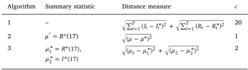
We implemented three ABC-rejection algorithms in R (Table 1). In thefirst, we used the daily counts of infected and recovered individuals from day 1 to day 17 to estimate our model parameters. The distance measure was the square root of the sum of squared differences of the number of infected and recovered individuals over time (Table 1).In the second, we assumed that the data consisted of the number of recovered individuals on day 17. Hence, our data isμ=R(17), and we calculate μ*

=R*(17) from our model simulations using the summary statistic i.e. the number of recovered individuals at the end of the model simulation. The distance measure between μandμ* _{was the square root of the} squared difference. In the third, we again assumed that the data con-sisted of the number of recovered individuals on day 17 but in addition, we also calculated the distance between the number of infected in-dividuals on day 17 and model predicted number.

The number of desired particles in all examples was chosen as N= 1000. We ran a pilot ABC-rejection algorithm with a smallerNand found that it was difficult to distinguish whether the lack of accuracy was from the small number of particles or the choice of summary sta-tistic. The tolerances were chosen to maximise the precision in esti-mation of model parameters. For thefirst example, we ran the ABC-rejection algorithm for a vector of tolerances to choose the tolerance which gave the smallest inter-quartile range of the model parameters (Figure S1). We chooseϵ= 20 as this had the smallest inter-quartile range. In principle, the tolerance could be much lower for thefirst example, but given the inefficient sampling of the model parameters, the run-time of the algorithm would be long. For examples two and Table 1

Description of the ABC-rejection algorithms implemented in R. Model simula-tions are denoted by*_.

Algorithm Summary statistic Distance measure ϵ

1 – _{∑ − + ∑ −}

= (I I*) = (R R*)

t T

t t t

T t t

1 2 1 2

20

2 μ*_=R*(17)

− μ μ

( *)2 1

3 μ₁*=R* (17),

= μ₂* I* (17)

− + −

μ μ μ μ

three, we choose the smallest possible tolerance for the model predic-tion. For example 2, this wasϵ= 1 (comparing the number of recovered individuals on day 17) and example 3, this wasϵ= 2 (comparing the number of recovered individuals and infected individuals on day 17). In all cases, we chose an informative prior for the initial number of sus-ceptibles and uniform priors for the model parameters (Table 2).

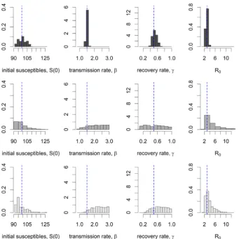
3.2. Results

The posterior estimates of the model parameters varied in accuracy and precision for the three ABC-rejection algorithms. When the data consisted of daily counts of infected and recovered individuals (ABC-rejection 1), the true model parameters were retrieved. When the data consisted of thefinal size if the epidemic (ABC-rejection 2), or of the

final size of the epidemic and number of infecteds at the end of the epidemic (ABC-rejection 3) then the posterior distribution of the transmission rate (β) was close to the Uniform prior distribution despite having very low tolerances. The posterior distribution for the recovery rate (γ) had a narrower distribution in rejection-3. In both ABC-rejection 2 and 3, the posterior of the basic reproduction number R0=β/γwas more accurate than the model parameters.

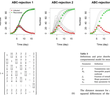
When the acceptance criteria consisted only of matching thefinal size of the epidemic (ABC-rejection 2) the accepted model parameters included epidemics which had not ended within the time frame of the true epidemic (Fig. 3). By adding the second criteria of matching the

final number of infecteds (0) then we see that the accepted model parameters gave epidemics which hadfinished within the time frame (Fig. 3). However, the model parameters could still be accepted where the transmission rate (β) was too high or the recovery rate (γ) was too low.

3.3. Case study 2: The 2004 measles outbreak in Malawi

3.3.1. Data and model

In this case study we have compared the performance of the ABC rejection and ABC-SMC algorithms using the 2010 measles outbreak in Malawi data and stochastic model with age structure. This example illustrates challenges to be expected when inferring parameters from a real-world data and a complex epidemic model.

In age-structured models, it is assumed that individuals within a particular age class exhibit more similar behaviour in comparison to other age classes. In the context of epidemiological modelling, infected individual has a higher probability of infecting susceptibles of the same age cohort. This is achieved by defining a Who Acquires Infection From Whom (WAIFW) matrix (Anderson and May, 1982). In this case study, we use the WAIFW matrix for measles from (Shea et al., 2014): Table 2

Definitions and prior distributions of the SIR model parameters.

Parameter Definition Prior distribution

β Transmission rate (day−1). Uniform (0, 3) γ Recovery rate (day−1). Uniform (0, 1) S0 Initial number of susceptibles. Pois (λ= 100)

= ⎡ ⎣ ⎢ ⎢ ⎢ ⎢ ⎢ ⎢ ⎢ ⎢ ⎢ ⎢ ⎢ ⎢ ⎢ ⎢ ⎢ ⎢ ⎢ … … … … … ⋮ ⋮ ⋮ ⋮ ⋮ ⋱ … ⎤ ⎦ ⎥ ⎥ ⎥ ⎥ ⎥ ⎥ ⎥ ⎥ ⎥ ⎥ ⎥ ⎥ ⎥ ⎥ ⎥ ⎥ ⎥ A 1 11 12 5 6 3 4 2 3 2 3 11 12 1 11 12 5 6 3 4 2 3 5 6 11 12 1 11 12 5 6 2 3 3 4 5 6 11 12 1 11 12 2 3 2 3 3 4 5 6 11 12 1 2 3 11 12 2 3 2 3 2 3 2 3 2

3 1 (6)

This is a symmetric matrix with it's values decreasing away from the main diagonal. We use a stochastic Susceptible-Exposed-Infected-Recovered (SEIR) model. The force of infection on an individual in age classiat timetis then given by:

∑

λ ti( ) β A I,

j i j j,

(7) whereβis transmission rate,Ijis the number of infectious individuals in

age classjandAi,jis the (i,j) element in the WAIFW matrix.

In this case study we will investigate the 2010 measles outbreak in Malawi (Minetti et al., 2013). The data consist of weekly cases and percentage of cases in three age groups (0.5–5 years, 5–15 and 15+ years). The cumulative number of cases during the outbreak was 134,000. We stratified the population into 22 age classes: 6–12 months, 1–2 years, 2–3 years,…, 19–20 years, and 20+ years; and assume that the age distribution of susceptible individuals in the population follows the Gamma(ash,art) distribution (Shea et al., 2014). We assume that all individuals 0–6 months old have maternal immunity (Caceres et al., 2000). The model is simulated using the tau-leaping algorithm with time intervals of one day (Gillespie, 2001).

The stochastic compartmental model with age-structure for measles has seven parameters. Duration of latent and infectious periods is seven days (Anderson and May, 1985). Therefore the number of parameters to be estimated isfive.

3.3.2. ABC setup

We chose uniform priors forfive model parameters (Table 3). As there are two different types of data describing the outbreak (i.e. temporal change in a number of cases and percentage of cases in three age groups), we use an intersection metrics in the ABC-SMC algorithm (McKinley et al., 2018). The distance measure for temporal data is the square root of the sum of squared differences of the number of weekly cases:

∑

= −

dT( ,D D*) (I I*) .

w

w w2

(8)

The distance measure for age data is the square root of the sum of squared differences of the percentage of infected individuals in the three age groups (0.5–5 years, 5–15 and 15+ years):

∑

∑

∑

dA( ,D D*) I/ I I*/ I* .

a a k k a k k 1 3 1 3 1 3 2 (9) We set the pair of thresholds {θT_,θA_{} for ABC rejection algorithm in}

the following way. If we desire the simulated number of cases to be within ± 20% of the observed number of cases during the outbreak

duration (i.e. 54 weeks), we get dT

= ∑ ₌ × =

D D I

( , *) _w 1(0.4 w*) 11, 900

54 ₂

. In a similar way, if we require the differences in each age group to be ± 1%, this gives

= × =

dA( ,D D*) 3 22 2.82_{. Therefore we setϵ}T

= 10, 000 andϵA= 3 for the ABC-rejection algorithm.

Next, we will investigate the performance of ABC-SMC algorithm. We will explore two strategies: (i) calculating covariance matrix using all sampled particles from the previous generation (ABC-SMC); and (ii) calculating covariance matrix usingMnearest neighbours of the par-ticleθg( )i−1(ABC-SMC MNN) (Filippi et al., 2013).

We set the same schedule of tolerances to run both the ABC-SMC and ABC-SMC MNN algorithms. For thefirst generation, we set the pair

of thresholds in the following way: as

= ∑ ₌ × =

dT( ,D D*) (2 I*) 59, 500

w 1 w

54 ₂

(i.e. we allow the discrepancy to be twice as large as weekly number of cases) and

= × =

dA( ,D D*) 3 102 17.32 _{(i.e. we allow the discrepancy to be as} large as ten percent for each age group), we set ϵT1 =50, 000 and

= ϵA 15

1 . Then we gradually decreased the threshold levels until they

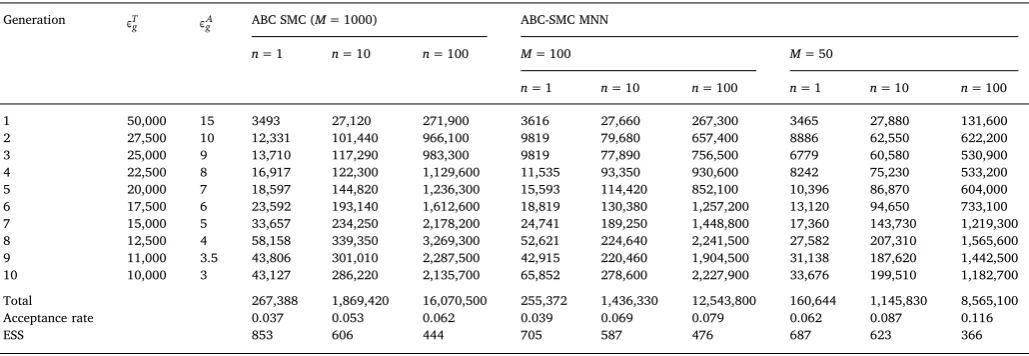
reached the samefixed level as was used for the ABC rejection method. The number of desired particles was set to N= 1000 and the number of generation to G= 10. The tolerance values for the last generation was set to be the same as for the ABC rejection algorithm. We have investigated how ABC-SMC and ABC-SMC MNN algorithms performed when a number of model runs for each parameter set was n= 1, n= 10 andn= 100. For ABC-SMC MNN method we set the number of neighbours toM= 50 andM= 100.

Finally, we tested the performance of ABC-SMC and ABC-SMC MNN by setting the new tolerances ϵgas a median (i.e. 50th quantile) of

Fig. 3.The true number of infected (red circle) and recovered individuals (green triangle) and SIR model simu-lations (shades of grey) using 10 ran-domly selected parameter sets from the posterior distributions inFig. 2. (For interpretation of the references to color in thisfigure legend, the reader is re-ferred to the web version of this ar-ticle.)

Table 3

Definitions and prior distributions of estimated parameters for stochastic compartmental model for measles.

Parameter Definition Prior distribution

β Transmission rate (day−1) Uniform (0, 5 × 10−6) N0 Susceptible population size before

outbreak

< ₋ dm( ,D D*) ϵ

g m

1 (McKinley et al., 2018). Again, thefinal generation

tolerance level was set to be equal or less then values used for the ABC rejection method.

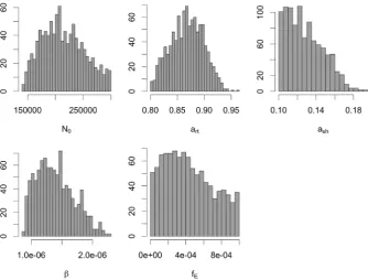
3.3.3. Results

First, we have employed the ABC rejection algorithm with toler-ancesϵT= 10, 000 andϵA= 3. The number of model runs required to obtain 1000 accepted particles was 29, 224, 520. This gives that the acceptance rate for the ABC rejection approach is 0.00003. The pos-terior estimates for the model parameters are shown inFig. 4(A)–(E). We have estimated mean value for the transmission rate equal to 1.39 × 10−6_{per day and range as (8.7 × 10}−7_{, 2.26 × 10}−6_).

Model simulations using 10 randomly selected parameter sets from the posterior distribution are shown inFig. 5. Demographic distribution of cases was calculated using these 10 simulations. There is a good agreement between the observed data and simulated data for both temporal dynamics of the outbreak and fraction of cases in three age groups.

Applying the ABC-SMC algorithm forG= 10 generations required one hundred times fewer model runs then the ABC-rejection algorithm: the total number of model runs required to obtain 1000 accepted

particles for the ABC-SMC was 267, 388. We have repeated parameter inference by re-running model 10 and 100 times for each proposed parameter set. The total number model runs to obtain 1000 accepted values for each generation is given inTable 4. For thefirst generation, where parameters are sampled from the prior distribution, the accep-tance rate was higher for multiple runs of the model (33.8% forn= 10 and 39.5% forn= 100) in comparison to a single model run (28.6%). The acceptance rates for generations 2–10 were as follows:n= 1 from 1.7% to 8.1% (ABC-SMC) and from 2.9% to 14.7% (ABC-SMC MNN); forn= 10 from 2.9% to 9.8% (ABC-SMC) and from 4.8% to 16.5% (ABC-SMC MNN); for n= 100 from 3.0% to 10.3% (ABC-SMC) and from 6.3% to 18.8% (ABC-SMC MNN). This result suggests that in-creasing a number of runs for each proposed parameter set increased parameter acceptance rate.

Using the multivariate normal kernel with 50 nearest neighbours increased the performance of the ABC-SMC algorithm. For example, the scheme required 160, 644 model runs in total in order to accept 1000 particles over 10 generations forn= 1, which gives around 40% re-duction in a number of simulations. When a number of nearest neigh-bours was set to 100, the ABC-SMC MNN algorithm showed improve-ment with respect to total number of runs in comparison to ABC-SMC, Fig. 4.The posterior distributions of parameters obtained using the ABC rejection algorithm.

but the performance was much lower whenM= 50.

We have investigated how ESS for the last generation compares for different configurations of the ABC algorithm. We found that the ESS values decreased when (i) number of nearest neighbours decreased; and (ii) number of model runs for each proposed parameter set increased. For the runs withn= 100, the ESS was below 500. In contrast, ac-ceptance rate calculated over all generations has increased when in-creasing number of model runs. Therefore, there is a trade-offbetween number of model runs, acceptance rate and variance of the weights of accepted particles when choosing a number of runs per proposed parameter set and number of nearest neighbours for covariance matrix of the perturbation kernel. Our analysis based on both the ABC-SMC and ABC-SMC NN indicates that havingn> 1 increases computation burden and decreases the ESS, which cannot be out-weighted by im-provement in the overall acceptance rate. This result is in agreement with McKinley et al. (McKinley et al., 2009), who found that for a given tolerance level, increasing the number of repeats did not produce markedly more precise posteriors.

Finally, we have explored the performance of the ABC-SMC and ABC-SMC MNN for the case when the tolerance is calculated as the median from the previous generation. Total number of model runs needed to accept N= 1000 particles in each generation is given in Table 5. All approaches required G= 7 generations to reach

<

ϵTg 10, 000 andϵgA<3.0. Using 50 nearest neighbours when

calcu-lating covariance matrix for perturbation kernel required 40% less model runs. Again, the increase in acceptance rate came at a cost of decreasing ESS.

3.4. Case study 3: Citrus tristeza virus spread in an orchard

3.4.1. Data and model

In this case study we will investigate the data based on small scale

field observations of citrus tristeza virus (CTV) spread in an orchard (Marcus et al., 1984). The trees were arranged in a rectangular frame, with an inter-row distance of 5.5 m and a between-column distance of 4 m. There were 131 infected trees in 1981 and 45 infected trees in 1982. Maps of susceptible and infected trees in 1981 and 1982 are shown inFig. 6. The virus affects citrus trees and is transmitted by the brown citrus aphid (Keeling and Rohani, 2007).

We model the spread of CTV using a spatio-temporal individual-based stochastic model. Each tree is classified as susceptible or infected. The force of infection on a susceptible tree i at time tis given by (Marcus et al., 1984; Keeling et al., 2004):

∑

∈

λ t( ) β K d

365 ( ),

i

j

i j infected

,

(10) whereβis yearly transmission rate,dijis the distance between treesi

and j, and K(d) =d−2α is a distance kernel. We have simulated a number of new cases every day for a year starting with the trees in-fected in 1981.

3.4.2. ABC setup

We implemented ABC algorithm with the distance measure which compares observed and simulated distribution of a minimal distance between trees infected in 1981 and 1982:

Table 4

Number of model runs needed to acceptN= 1000 particles in each generation, acceptance rate and ESS for ABC algorithms run with afixed set of tolerances. Generation _ϵ

g

T _ϵ

gA ABC SMC (M= 1000) ABC-SMC MNN

n= 1 n= 10 n= 100 M= 100 M= 50

n= 1 n= 10 n= 100 n= 1 n= 10 n= 100

1 50,000 15 3493 27,120 271,900 3616 27,660 267,300 3465 27,880 131,600

2 27,500 10 12,331 101,440 966,100 9819 79,680 657,400 8886 62,550 622,200

3 25,000 9 13,710 117,290 983,300 9819 77,890 756,500 6779 60,580 530,900

4 22,500 8 16,917 122,300 1,129,600 11,535 93,350 930,600 8242 75,230 533,200

5 20,000 7 18,597 144,820 1,236,300 15,593 114,420 852,100 10,396 86,870 604,000 6 17,500 6 23,592 193,140 1,612,600 18,819 130,380 1,257,200 13,120 94,650 733,100 7 15,000 5 33,657 234,250 2,178,200 24,741 189,250 1,448,800 17,360 143,730 1,219,300 8 12,500 4 58,158 339,350 3,269,300 52,621 224,640 2,241,500 27,582 207,310 1,565,600 9 11,000 3.5 43,806 301,010 2,287,500 42,915 220,460 1,904,500 31,138 187,620 1,442,500 10 10,000 3 43,127 286,220 2,135,700 65,852 278,600 2,227,900 33,676 199,510 1,182,700

Total 267,388 1,869,420 16,070,500 255,372 1,436,330 12,543,800 160,644 1,145,830 8,565,100

Acceptance rate 0.037 0.053 0.062 0.039 0.069 0.079 0.062 0.087 0.116

ESS 853 606 444 705 587 476 687 623 366

Table 5

Number of model runs needed to acceptN= 1000 particles in each generation, acceptance rate and ESS for ABC algorithms run with tolerances calculated from previous generation (n= 1).

Generation ABC-SMC ABC-SMC MNN

ϵgT ϵgA M= 100 M= 50

ϵTg ϵgA ϵgT ϵgA

2 67,160 8.21 4,404 62,885 8.45 4705 67,160 8.21 4450

3 29,749 5.39 11,301 29,749 5.38 7696 30,705 5.34 6405

4 27,490 4.20 29,494 26,422 4.11 18,456 26,612 4.07 16,843

5 17,837 3.59 40,658 17,585 3.34 25,863 16,965 3.40 20,476

6 12,550 3.14 74,170 12,514 2.90 52,082 12,199 2.93 35,891

7 9687 2.84 84,400 9591 2.68 71,236 9782 2.67 61,315

Total 245,427 181,038 146,380

Acceptance rate 0.028 0.038 0.047

∑

= −

∈

d D DS( , *) (n ( )δ n ( )) ,δ

δ Δ

obs sim 2

(11) whereΔis a set of all distances between trees. There are 992 unique distances between all trees. A number of observed and simulated minimal distances is calculated as:

∑

= − =

n δ( ) (min ||a b|| δ), ₍₁₂₎

wherea are the coordinates of trees infected in 1981 (i.e. observed incidences of disease); and bare the coordinates of trees infected in 1982 (i.e. observed or simulates incidences of disease).

The number of desired particles wasN= 1000. If we assume that there were no new cases in 1982, we get thatdS_(D,D*_{) = 20. Therefore} we choseϵ1= 20. There were 45 infected trees in 1982, therefor we required that the threshold for the last generation would be less then

=

45/2 4.74. The schedule of tolerances was then set toϵ= 20, 15, 10, 7.5, 6, 5, 4.5.

We have investigated how ABC SMC MNN algorithm performed when covariance matrix of the perturbation kernel was calculated using M= 1000, M= 500, M= 100 and M= 50 of nearest neighbours. Parameter priors are given inTable 6.

3.4.3. Results

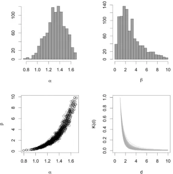
First, we implemented ABC-SMC MNN withM= 50.Fig. 7shows the posterior distributions of the model parameters andfitted distance kernel. We estimated the mean of power law decay parameter to be 1.32. The value previously identified by MCMC analysis is α= 1.3 (Gibson, 1997) and using conservation of pattern method α= 1.35 (Keeling et al., 2004).

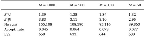
Model simulations using 100 randomly selected parameter sets from the posterior distribution are shown inFig. 8. It can be seen that the mean number of simulated infections within a year (41.5 cases) is close to the observed number of new infections (45 cases). The distributions of simulated number of minimal distances lie close to the observed number of minimal distances, as expected. Figure on the bottom shows a proportion of simulations which had a tree being infected at the start of 1982 with darker shades illustrating a higher number of simulations. Performance of ABC SMC MNN algorithm implemented using M= 1000,M= 500,M= 100 andM= 50 is given in Table 7. The mean of power law decay parameter decreased from 1.39 to 1.35 when M decreased. We have found that decreasing number of neighbour particles decreases number of model runs required to accept 1000 particles and increases parameter acceptance rate. However, the ESS

values for the last generation were at the similar level (630–650). For a comparison, we have employed the ABC rejection algorithm with toleranceϵ= 4.5. The mean of power law decay parameter was 1.39, i.e. similar to the result withM= 1000. The number of model runs required to obtain 1000 accepted particles was 3, 820, 136. This gives that the acceptance rate for the ABC rejection approach is 0.00026.

4. Discussion

The purpose of this paper was to provide an introductory tutorial in using ABC for infectious disease modelling. We have introduced the user choices required to implement the ABC-rejection algorithm and the ABC-SMC algorithm. These user defined choices can be model or data based. In addition, with larger data sets and more complex models, there are also computational trade-offs to be made, such as with a more sophisticated ABC algorithm. Here, we have presented three case stu-dies to illustrate how to implement ABC-rejection and ABC-SMC in R. However, there are numerous applications and examples which we have not covered but have been by other authors. We have applied the ABC-SMC algorithm to stochastic models, but the technique has been used for a system of ordinary differential equations as well (Toni et al., 2009; Filippi et al., 2013).

In case study 1 we illustrated the information lost and the changes that need to be made to the algorithm based on different resolutions of data. Daily counts of infected and recovered individuals provides en-ough information to re-estimate model parameters. However, when the number of recovered or infected individuals was known, only the basic reproduction number can be re-estimated and with less precision. This is due to the lack of temporal information in the data and the correla-tion between the transmission rate and recovery rate. If the user was able to specify an informative prior for either the transmission rate or recovery rate, then the other parameter could be estimated.

The ABC-rejection algorithm has inefficient sampling in comparison to the ABC-SMC algorithm. By re-sampling from a smaller generation and slowly decreasing tolerance, we saw that in case study 2, ABC-SMC required hundred times fewer model runs then the ABC-rejection al-gorithm: the number of model runs required to obtain 1000 accepted particles for ABC rejection algorithm was 29, 224, 520, while for ABC-SMC it was 267, 388. Furthermore, if only 50 nearest neighbours of particles were used to parametrise the perturbation kernel, the number of model runs was reduced to 160, 644. Running the model for each proposed parameter set more times resulted in a higher acceptance rate. However, the trade-offbetween running model multiple times and in-creasing acceptance rate will depend on a cost of each model run and decreased effective sample size. For case study 3, decreasing number of neighbour particles decreased number of model runs and increased parameter acceptance rate, but had no effect on values of effective sample size.

The number of desired particles in all case studies was set to Fig. 6.Locations of trees: susceptible trees (green circles) and trees infected by CTV (red circles) (Marcus et al., 1984). (For interpretation of the references to color in thisfigure legend, the reader is referred to the web version of this article.)

Table 6

Definitions and prior distributions of estimated parameters.

Parameter Definition Prior distribution

α Power law decay. Uniform (0, 5)

Fig. 7.The posterior distributions of the model parameters andfitted distance kernel.

N= 1000 as in (Toni et al., 2009). The choice of number of particles will affect the speed of the ABC algorithm and the accuracy of thefinal posterior distribution. Additionally, the magnitude of the tolerance will also affect the speed of the algorithm and accuracy of the algorithm. The choice of tolerance in the ABC-rejection algorithm can be informed by trial and error. In the ABC-SMC algorithm, instead of proposing a vector of tolerances, the tolerance at each population can be calculated as theαquantile of the distances of the accepted particles (Prangle, 2017). The user then has to choose some quantile (q) and the number of populations (G). This quantile method means that the user does not need to supply a vector of tolerances, however must choose the number of populations (G). Convergence can be assessed by the difference using the inter-quartile ranges of the values of accepted particles as a measure of goodness offit between successive intermediate distributions (Toni et al., 2009).

Exploration of the data is also essential to inform the choice of summary statistics. In all cases we have used a distance measure as the squared difference between observed and simulated data. Other options are available as the absolute difference (Sunnåker et al., 2013). If the model output is a two peak epidemic then an appropriate summary statistic may be to match the time of the two peaks, or the ratio of the size of one peak to another. Distance can include summary statistics which is a function of model outputs only, for example, simulated in-fection pressures (Prangle et al., 2018). Proposed solutions to choosing optimal summary statistics for ABC include a sequential scheme to as-sess the information content of a list of summary statistics (Joyce and Marjoram, 2008), minimisation of the estimated entropy of the pos-terior approximation (Nunes and Balding, 2010), finding statistical summaries of the data that minimise the loss of information (Barnes et al., 2012), constructing summary statistics as estimates of the pos-terior mean of the parameters (Fearnhead and Prangle, 2012), or em-ploying a machine learning tool named random forests where a re-ference table generated from a prior distribution is used to train regression trees (Pudlo et al., 2015; Raynal et al., 2018). We re-commend looking at the literature for inspiration the user defined choices including the summary statistics. The type of data available and problems which arise from infectious disease modelling reoccur in the literature. For a review of applications of ABC seeBeaumont (2010)and the papers highlighted in the discussion. Also for applications of ABC-SMC in infectious disease modelling seeConlan et al. (2012),Hladish et al. (2018).

In this paper, we have assumed that the user is writing their ABC algorithm in computer code. There are R packages which implement ABC algorithms: abc(ABC-rejection method) (Csilléry et al., 2012), abctools (ABC-rejection method) (Nunes and Prangle, 2015), abcrf (ABC parameter inference via random forests) (Raynal et al., 2018), and easyABC(ABC-rejection and ABC-SMC methods) (Jabot et al., 2013). While learning the steps of ABC, the authors believe that the user is more likely to understand each step of the algorithm with code, in comparison to a package. In addition, by writing the full ABC algorithm in code, the user has theflexibility to alter steps according to their type of model and their data. However, there are some simple applications of ABC where a package would be appropriate if that is the user's pre-ference. We hope that the case studies we presented here can give practically useful insight when making various ABC algorithm tuning choices.

ABC is a powerful tool but an ABC algorithm must be tailored to the model and data at hand. The performance of any modelfitting algo-rithm is restricted by the available data which the user is trying tofit their model to. The user must specify a model appropriate for their data source, i.e. parameters must all be identifiable from the data at hand. If the model is stochastic, investigating the variability in the model output for the same set of parameter values will inform how the choice ofn, the number of times to run the model and also what summary statistics to choose. By simulating data from the model, and attempting to re-esti-mate the known parameters the user can identify changes that are needed for their question specific ABC algorithm.

Conflicts of interest

The authors have no conflicts of interest to declare. Acknowledgements

We would like to thank Will Probert for his comments on the manuscript and the reproducibility of the code. The authors thank the UK National Institute for Health Research Health Protection Research Unit (NIHR HPRU) in Modelling Methodology at Imperial College London in partnership with Public Health England (PHE) for funding (grant HPRU-2012–10080).

Appendix A. Supplementary data

Supplementary data associated with this article can be found, in the online version, athttps://doi.org/10.1016/j.epidem.2019.100368. References

Anderson, R., May, R., 1982. Control of communicable disease by age-specific im-munisation schedules. Lancet 319 (8264), 160.

Anderson, R.M., May, R.M., 1985. Age-related changes in the rate of disease transmission: implications for the design of vaccination programmes. J. Hyg. 94 (03), 365–436. Anderson, R.M., May, R.M., 1991. Infectious Diseases of Humans, 1st ed. Oxford

University Press.

Babad, H.R., Nokes, D.J., Gay, N.J., Miller, E., Morgan-Capner, P., Anderson, R.M., 1995. Predicting the impact of measles vaccination in England and Wales: model validation and analysis of policy options. Epidemiol. Infect. 114 (02), 319.

Baragatti, M., Pudlo, P., 2014. An overview on approximate Bayesian computation. ESAIM: PROCEEDINGS 44, 291–299.

Barnes, C.P., Filippi, S., Stumpf, M.P.H., Thorne, T., 2012. Considerate approaches to constructing summary statistics for ABC model selection. Stat. Comput. 22 (6), 1181–1197.

Beaumont, M.A., 2010. Approximate Bayesian computation in evolution and ecology. Annu. Rev. Ecol. Evolut. Syst. 41 (1), 379–406.

Beaumont, M.A., Zhang, W., Balding, D.J., 2002. Approximate Bayesian computation in population genetics. Genetics 162 (4), 2025–2035.

Caceres, V.M., Strebel, P.M., Sutter, R.W., 2000. Factors determining prevalence of ma-ternal antibody to measles virus throughout infancy: a review. Clin. Infect. Dis. 31 (1), 110–119.

Campbell, P.T., McCaw, J.M., McVernon, J., 2015. Pertussis models to inform vaccine policy. Hum. Vaccines Immunother. 11 (3), 669–678.

Chapman, L.A.C., Jewell, C.P., Spencer, S.E.F., Pellis, L., Datta, S., Chowdhury, R., Bern, C., Medley, G.F., Hollingsworth, T.D., 2018. The role of case proximity in transmis-sion of visceral leishmaniasis in a highly endemic village in Bangladesh. PLOS Negl. Trop. Dis. 12 (10), e0006453.

Conlan, A.J.K., McKinley, T.J., Karolemeas, K., Pollock, E.B., Goodchild, A.V., Mitchell, A.P., Birch, C.P.D., Clifton-Hadley, R.S., Wood, J.L.N., 2012. Estimating the hidden burden of bovine tuberculosis in Great Britain. PLOS Comput. Biol. 8 (10), 1–14. Csilléry, K., François, O., Blum, M.G.B., 2012. abc: an r package for approximate Bayesian

computation (ABC). Methods Ecol. Evolut. 3 (3), 475–479.

Fearnhead, P., Prangle, D., 2012. Constructing summary statistics for approximate Bayesian computation: semi-automatic approximate Bayesian computation. J. R. Stat. Soc. Ser. B (Stat. Methodol.) 74 (3), 419–474.

Filippi, S., Barnes, C.P., Cornebise, J., Stumpf, M.P., 2013. On optimality of kernels for approximate Bayesian computation using sequential Monte Carlo. Stat. Appl. Genet. Mol. Biol. 12 (1).

Gelman, A., Carlin, J.B., Stern, H.S., Rubin, D.B., 2013. Bayesian Data Analysis, 3rd ed. Chapman and Hall/CRC.

Gibson, G.J., 1997. Markov chain monte carlo methods forfitting spatiotemporal sto-chastic models in plant epidemiology. J. R. Stat. Soc. Ser. C (Appl. Stat.) 46 (2), 215–233.

Gillespie, D.T., 2001. Approximate accelerated stochastic simulation of chemically Table 7

Comparison of ABC SMC MNN algorithms.

M= 1000 M= 500 M= 100 M= 50

E[λ] 1.39 1.35 1.34 1.32

E[β] 3.83 3.11 3.10 2.95

No runs 155,108 108,590 95,116 89,863

Accept. rate 0.045 0.064 0.073 0.077

reacting systems. J. Chem. Phys. 115 (4), 1716–1733.

Hartig, F., Calabrese, J.M., Reineking, B., Wiegand, T., Huth, A., 2002. Statistical in-ference for stochastic simulation models–theory and application. Ecol. Lett. 14 (8), 816–827.

Hill, E.M., House, T., Dhingra, M.S., Kalpravidh, W., Morzaria, S., Osmani, M.G., Yamage, M., Xiao, X., Gilbert, M., Tildesley, M.J., 2017. Modelling h5n1 in bangladesh across spatial scales: model complexity and zoonotic transmission risk. Epidemics 20, 37–55.

Hladish, T.J., Pearson, C.A.B., Patricia Rojas, D., Gomez-Dantes, H., Halloran, M.E., Vazquez-Prokopec, G.M., Longini, I.M., 2018. Forecasting the effectiveness of indoor residual spraying for reducing dengue burden. PLOS Negl. Trop. Dis. 12 (6), 1–16. Jabot, F., Faure, T., Dumoulin, N., 2013. EasyABC: performing efficient approximate

Bayesian computation sampling schemes using r. Methods Ecol. Evolut. 4 (7), 684–687.

Joyce, P., Marjoram, P., 2008. Approximately sufficient statistics and Bayesian compu-tation. Stat. Appl. Genet. Mol. Biol. 7 (1).

Kanaan, M.N., Farrington, C.P., 2005. Matrix models for childhood infections: a Bayesian approach with applications to rubella and mumps. Epidemiol. Infect. 133 (06), 1009. Keeling, M.J., Brooks, S.P., Gilligan, C.A., 2004. Using conservation of pattern to estimate

spatial parameters from a single snapshot. Proc. Natl. Acad. Sci. USA 101 (24), 9155–9160.

Keeling, M.J., Rohani, P., 2007. Modeling Infectious Diseases in Humans and Animals, 1st ed. Princeton University Press, Princeton, N.J.

Keeling, M.J., Woolhouse, M.E.J., Shaw, D.J., Matthews, L., Chase-Topping, M., Haydon, D.T., Cornell, S.J., Kappey, J., Wilesmith, J., Grenfell, B.T., 2001. Dynamics of the 2001 UK foot and mouth epidemic: stochastic dispersal in a heterogeneous landscape. Science 294 (5543), 813–817.

Kypraios, T., Neal, P., Prangle, D., 2017. A tutorial introduction to Bayesian inference for stochastic epidemic models using approximate Bayesian Computation. Math. Biosci. 287, 42–53.

Lenormand, M., Jabot, F., Deffuant, G., 2013. Adaptive approximate Bayesian computa-tion for complex models. Comput. Stat. 28 (6), 2777–2796.

Marcus, R., Fishman, S., Talpaz, H., Salomon, R., Bar-Joseph, M., 1984. On the spatial distribution of citrus tristeza virus disease. Phytoparasitica 12 (1), 45–52. Marjoram, P., Molitor, J., Plagnol, V., Tavaré, S., 2003. Markov chain Monte Carlo

without likelihoods. Proc. Natl. Acad. Sci. USA 100 (26), 15324–15328. McKinley, T., Cook, A.R., Deardon, R., 2009. Inference in epidemic models without

likelihoods. Int. J. Biostat. 5 (1).

McKinley, T.J., Vernon, I., Andrianakis, I., McCreesh, N., Oakley, J.E., Nsubuga, R.N., Goldstein, M., White, R.G., 2018. Approximate Bayesian computation and simula-tion-based inference for complex stochastic epidemic models. Stat. Sci. 33 (1), 4–18.

Minetti, A., Kagoli, M., Katsulukuta, A., Huerga, H., Featherstone, A., Chiotcha, H., Noel, D., Bopp, C., Sury, L., Fricke, R., Iscla, M., Hurtado, N., Ducomble, T., Nicholas, S., Kabuluzi, S., Grais, R.F., Luquero, F.J., 2013. Lessons and challenges for measles control from unexpected large outbreak, Malawi. Emerg. Infect. Dis. 19 (2), 202–209. Moral, P.D., Doucet, A., Jasra, A., 2011. An adaptive sequential monte carlo method for

approximate Bayesian computation. Stat. Comput. 22 (5), 1009–1020. Nunes, M.A., Balding, D.J., 2010. On optimal selection of summary statistics for

ap-proximate Bayesian computation. Stat. Appl. Genet. Mol. Biol. 9 (1).

Nunes, M.A., Prangle, D., 2015. abctools: an R package for tuning approximate Bayesian computation analyses. R Journal 7 (2), 189–205.

Perez-Lezaun, A., Pritchard, J.K., Seielstad, M.T., Feldman, M.W., 1999. Population growth of human Y chromosomes: a study of Y chromosome microsatellites. Mol. Biol. Evolut. 16 (12), 1791–1798.

Prangle, D., 2014. Lazy ABC. Stat. Comput. 26 (1–2), 171–185.

Prangle, D., 2017. Adapting the abc distance function. Bayesian Anal. 12 (1), 289–309. Prangle, D., Everitt, R.G., Kypraios, T., 2018. A rare event approach to high-dimensional

approximate Bayesian computation. Stat. Comput. 28 (4), 819–834. Pudlo, P., Marin, J.-M., Estoup, A., Cornuet, J.-M., Gautier, M., Robert, C.P., 2015.

Reliable ABC model choice via random forests. Bioinformatics 32 (6), 859–866. Raynal, L., Marin, J.-M., Pudlo, P., Ribatet, M., Robert, C.P., Estoup, A., 2018. ABC

random forests for Bayesian parameter inference. Bioinformatics.

Sadegh, M., Vrugt, J.A., 2014. Approximate Bayesian computation using markov chain monte carlo simulation: dream(abc). Water Resour. Res. 50 (8), 6767–6787. Schuette, M., 1999. Modeling the effects of varicella vaccination programs on the

in-cidence of chickenpox and shingles. Bull. Math. Biol. 61 (6), 1031–1064. Shea, K., Tildesley, M.J., Runge, M.C., Fonnesbeck, C.J., Ferrari, M.J., 2014. Adaptive

management and the value of information: learning via intervention in epidemiology. PLOS Biol. 12 (10), e1001970.

Sunnåker, M., Busetto, A.G., Numminen, E., Corander, J., Foll, M., Dessimoz, C., 2013. Approximate Bayesian computation. PLOS Comput. Biol. 9 (1), 1–10.

Toni, T., Welch, D., Strelkowa, N., Ipsen, A., Stumpf, M.P., 2009. Approximate Bayesian computation scheme for parameter inference and model selection in dynamical sys-tems. J. R. Soc. Interface 6 (31), 187–202.

Visser, M.D., McMahon, S.M., Merow, C., Dixon, P.M., Record, S., Jongejans, E., 2015. Speeding up ecological and evolutionary computations in R; essentials of high per-formance computing for biologists. PLOS Comput. Biol. 11 (3), 1–11.