Minmax Regret Combinatorial Optimization
Problems with Ellipsoidal Uncertainty Sets
∗
Andr´
e Chassein
†1and Marc Goerigk
‡21
Fachbereich Mathematik, Technische Universit¨at Kaiserslautern, Germany 2Department of Management Science, Lancaster University, United Kingdom
Abstract
We consider robust counterparts of uncertain combinatorial optimiza-tion problems, where the difference to the best possible soluoptimiza-tion over all scenarios is to be minimized. Such minmax regret problems are typically harder to solve than their nominal, non-robust counterparts. While cur-rent literature almost exclusively focuses on simple uncertainty sets that are either finite or hyperboxes, we consider problems with more flexible and realistic ellipsoidal uncertainty sets. We present complexity results for the unconstrained combinatorial optimization problem, the shortest path problem, and the minimum spanning tree problem. To solve such prob-lems, two types of cuts are introduced, and compared in a computational experiment.
Keywords: robust optimization; minmax regret; ellipsoidal uncertainty; complexity; scenario relaxation
1
Introduction
We consider general combinatorial optimization problems of the form
min{cTx:x∈ X ⊆ {0,1}n}
where the objective vector c is unknown, and coming from a set U of possible realizations. To find a solution x that still performs well under all possible outcomes ofc, several robust optimization approaches have been developed (for an overview, we refer to [GS16, BBC11, CG16]).
In this paper, we focus on the minmax regret approach, which is amongst the best-established methods in robust optimization [IS95, KY97, ABV09]. The
∗Effort sponsored by the Air Force Office of Scientific Research, Air Force Material
Com-mand, USAF, under grant number FA8655-13-1-3066. The U.S Government is authorized to reproduce and distribute reprints for Governmental purpose notwithstanding any copyright notation thereon.
†Email: [email protected]
basic idea is to find a solution that minimizes the largest difference to the opti-mal objective value in each scenario. More foropti-mally, we use a robust objective function of the form
Reg(x,U) = max{cTx−opt(c) :c∈ U }
with opt(c) being the optimal objective value of the original problem with ob-jective vectorc, and aim at solving the minmax regret problem
min{Reg(x,U) :x∈ X }
This problem has been extensively analyzed for finite and hyperbox uncertainty sets. Most minmax regret problems of this kind are NP-hard, see., e.g., [AL05, ABV05, Ave01] and the overview in [ABV09]. Therefore, both approximation algorithms and heuristic algorithms without performance guarantees have been suggested.
[KZ06] showed that solving the midpoint scenario of an interval uncertainty set gives a 2-approximation for minmax regret combinatorial optimization prob-lems. This was further extended in [Con12] to symmetry points of general un-certainty sets. In [CG15], an a-posteriori bound for the midpoint solution was presented, which can be used in a branch-and-bound algorithm.
[MGD04] developed a branch-and-bound algorithm for robust spanning trees. For the same problem, also a scenario relaxation procedure was presented in [PGAMCVT14]. The basic idea of scenario relaxation is to begin with a finite subset of scenarios, instead of the whole interval set. Then, worst-case scenar-ios are iteratively added to the scenario set, until the objective value of this relaxation coincides with the actual objective value of the regret problem with intervals.
Quite surprisingly, little attention has been paid to uncertainty sets that are not finite or hyperboxes. It seems that this is at odds with the development of other approaches to robust optimization, where the use of more sophisticated sets has been of primary importance. We mention ellipsoidal uncertainty sets (see [BTGN09]) and Γ-uncertainty sets (see [BS04]) as the most prominent examples.
There are several reasons to use ellipsoidal uncertainty sets in robust opti-mization. First, they give good tractability results for other robust optimization approaches. So far, this question is open for minmax regret. Second, they are flexible, as the generalized∩-ellipsoidal uncertainty introduced in [BTN98] even incorporates finite (via their convex hull) and interval sets. Third, they are well-motivated from a stochastic setting, where they naturally occur when a normal distribution is cut off at a certain level of probability.
In this paper we consider ellipsoidal uncertainty sets in minmax regret prob-lems. To the best of our knowledge, there is only one previous paper that also considers this type of problem [TTT10]. There, the authors consider uncertain convex quadratic problems and present a relaxation heuristic with probabil-ity guarantees. In this paper, we focus on combinatorial problems, complexprobabil-ity results and exact solution algorithms.
in polynomial time, we find the surprising result that the reverse holds true for axis-parallel ellipsoids: While it is NP-hard to compute the regret objective of one candidate solution, the optimal solution of the problem can be found in polynomial time.
In Section 3, we discuss two different ways to reformulate the minmax regret problem via a scenario relaxation procedure, resulting in exact, general solution approaches. These algorithms are compared in computational experiments in Section 4. Final conclusions are drawn and further research directions are posted in Section 5.
2
Complexity Results
2.1
Problem Definition
We consider combinatorial optimization problems to investigate the computa-tional complexity of the minmax regret problem for different uncertainty sets. We consider the cases of
• interval or hyperbox uncertaintyU =
×
ni=1[ˆci−di,ˆci+di], wheredi≥0,• axis-parallel ellipsoidsU ={c: (c−ˆc)TD(c−cˆ)≤1}, where D0 is a
positive definite diagonal matrix,
• general ellipsoidsU ={cˆ+Cξ:kξk2≤1}, and
• finite uncertainty setsU ={c1, . . . , ck}, wherekis polynomially bounded. Note that each axis-parallel ellipsoid can be expressed as a general ellipsoid. For each uncertainty set we study the complexity of solving the minmax regret problem, i.e., finding the optimal solution of
min
x∈XReg(x,U) = minx∈Xmaxc∈U
cTx−min
y∈Xc
Ty
(Solve)
and evaluating the regret of a given solution, i.e., computing the value of
Reg(x,U) = max
c∈U
cTx−min
y∈Xc
Ty
. (Eval)
The unconstrained combinatorial problem is the simplest non-trivial com-binatorial problem. The feasible set X ={0,1}n is the set of all 0,1-vectors.
We denote this problem as (U P). The shortest path problem is one of the most studied combinatorial problems. Each vectorxin the feasible setX is an incidence vector of ans−tpath in a graphG. This problem is denoted as (SP). Additionally, we briefly sketch how results for (SP) can be transferred to the minimum spanning tree problem (M ST).
Some of the presented reductions use the NP-complete partition problem: Given a list of natural numbersa1, . . . , an. The problem is to decide if a subset
I⊂ {1, . . . , n}of the index set exists such thatP
i∈Iai = P
i /∈Iai.
Lemma 1. (See [BTN99]) For an ellipsoidal uncertainty set U = {Cξ + ˆc :
kξk2≤1}, it holds that
max
c∈U c
Tx= ˆcTx+kCTxk
2. (1)
In case of an axis-parallel ellipsoid, Lemma 1 becomes:
Lemma 2. For an axis-parallel ellipsoidal uncertainty setU ={c: (c−ˆc)TD(c−
ˆ
c)T ≤1}, it holds that
max
c∈U c
Tx= ˆcTx+
v u u t n X i=1
D−ii1x2
i (2)
2.2
The Unconstrained Combinatorial Problem
Robust counterparts of the unconstrained combinatorial problem were first con-sidered in [BBI14], where it was shown that the minmax counterpart
min
x∈{0,1}nmaxc∈U c
Tx
is NP-hard already for an uncertainty set consisting only of two scenarios. To the best of our knowledge, no complexity results have been provided for the minmax regret counterpart. For the sake of completeness, we therefore also consider the complexity for interval and finite sets in this section.
We first consider the evaluation problem of (U P). For interval uncertainty and finite uncertainty, evaluating a solution is simple, as the following two the-orems demonstrate.
Theorem 1. The evaluation problem of (U P) for interval uncertainty sets is
in P.
Proof. The evaluation problem is given by
max
c∈U
cTx−min
y∈Xc
T y
= max
c∈U c
T
x−
n X
i=1
min(0, ci) !
=
n X
i=1
c∗i(xi)xi−
n X
i=1
min(0, c∗i(xi))
(3)
with c∗i(xi) = ˆci+ (2xi−1)di. For fixed x this expression can be computed
in O(n).
Theorem 2. The evaluation problem of(U P)for finite uncertainty sets is inP.
Proof. The evaluation problem is given by
max
c∈U
cTx−min
y∈Xc
Ty
= max
c∈U c
Tx−
n X
i=1
min(0, ci) !
= max
j=1,...,k n X
i=1
cjixi−
n X
i=1
min(0, cji)
!
We now turn to the more involved case of ellipsoidal uncertainty sets. Here, evaluating a solution is already a hard problem, as the following theorem shows.
Theorem 3. The evaluation problem of (U P) for axis-parallel ellipsoidal
un-certainty sets isNP-complete.
Proof. We give a reduction from the partition problem.
The axis-parallel ellipsoidal uncertainty set U is defined by the midpoint vector ˆcand diagonal matrixD. We set ˆci= 2aiandDii =8Aa1
i fori= 1, . . . , n
andA=Pn
i=1ai. Consider the evaluation problem forx= 0:
max
c∈U
cTx−min
y∈Xc
Ty
= max
c∈U
0−min
y∈Xc
Ty
= max
c∈U maxy∈Xc
T(−y)
= max
y∈X maxc∈U c
T(
−y)
Eq. (2) = max y∈X n X i=1
2ai(−yi) + v u u t n X i=1
8Aai(−yi)2
=−min
y∈X
n X
i=1
2aiyi− v u u t n X i=1
8Aaiyi
Define for each solutiony ∈ X the value λy := A1
Pn
i=1aiyi ∈[0,1]. Note
that the objective value of the minimization problem can be expressed usingλy
n X
i=1
2aiyi− v u u t n X i=1
8Aaiyi= 2Aλy− q
8A2λ
y
Consider the functionf : [0,1]→R, f(λ) = 2Aλ−√8A2λ. The minimum
of this function is attained forλ∗= 0.5 due to the first order condition, further
f(λ∗) =−A. This observation proves that the regret for x= 0 is at least Aif and only if the partition instance is a yes-instance.
As a direct consequence of Theorem 3, we also have that the general case is
NP-complete.
Corollary 1. The evaluation problem of (U P) for general ellipsoidal
uncer-tainty sets is NP-complete.
Having established the complexity of the evaluation problem, we now turn to the solution problem. We first consider the complexity for finite uncertainty sets.
Theorem 4. The solution problem of (U P) for finite uncertainty sets is NP -complete.
Proof. Again we use a reduction from partition. The uncertainty set consists
of only two scenarios c1 = (a
1, . . . , an) and c2 = (−a1, . . . ,−an). Denote by
A=Pn
i=1ai. We claim that a solution with regret at most
A
if the partition instance is a yes-instance. LetIbe the solution of the partition instance. We define solutionx∗i = 1 ∀i∈I andx∗i = 0∀i /∈I. The regret ofx∗
is given by
max(X
i∈I
ai,−
X
i∈I
ai+A) = max( X
i∈I
ai,
X
i /∈I
ai) =
A
2.
Conversely, let a solution xwith regret at most A2 be given. LetS ={i:xi=
1, i= 1, . . . , n}. The regret ofxis given by
max(X
i∈S
ai,−
X
i∈S
ai+A) = max( X
i∈S
ai,
X
i /∈S
ai)≥
A
2.
Since the regret ofxis at most A
2, we know that the regret of xis exactly
A
2.
Therefore, max(P
i∈Sai,Pi /∈Sai) = A2, which proves that S is a solution for
the partition instance.
Instead of considering the case of interval and axis-parallel ellipsoid un-certainty sets separately, we directly consider the more general case of
axis-symmetric uncertainty sets. A set U is axis-symmetric if it exists a midpoint
ˆ
c ∈ U such that for any c ∈ U with c = ˆc+γ for any index i it holds that
ci :=c−2γiei ∈ U where ei is the ith unit vector. Prominent axis-symmetric
uncertainty sets are interval, axis-parallel ellipsoids, or Γ−uncertainty sets.
Theorem 5. The midpoint solution
ˆ
x∈arg min{cˆTx:x∈ X }
is an optimal solution of (U P)for axis-symmetric uncertainty sets.
Proof. We define ˆxi = 1 if and only if ˆci ≤ 0. The goal is to show that ˆx is
optimal for the minmax regret problem. Let x∗ be an optimal solution with
x∗i = 1 and ˆci>0 for somei. In the following we show thatx0 =x∗−ei is also
an optimal solution.
Reg(x0) = max
c∈U maxy∈Xc
T(x0−y)
= max
c∈U c
Tx0−
n X
i=1
min(0, ci) !
=c0Tx0−
n X
i=1
min(0, c0i)
= ˆcTx0+γ0Tx0−
n X
i=1
min(0,ˆci+γi0)
where c0 is the worst case scenario (for the regret objective function) andc0 = ˆ
c+γ0. We define ˜γj =γj0 ∀j6=iand ˜γi=−γi0. We claim that
ˆ
cTx0+γ0Tx0−
n X
i=1
min(0,cˆi+γi0)≤cˆ
Tx∗+ ˜γTx∗−
n X
i=1
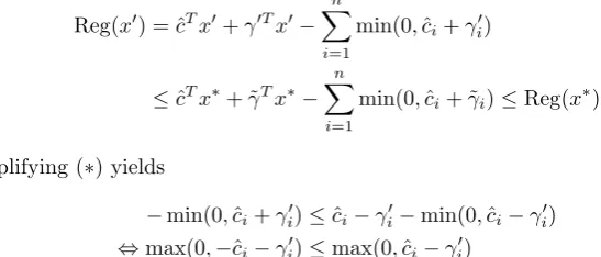
Using (∗) we can show thatx0 is also an optimal solution, since
Reg(x0) = ˆcTx0+γ0Tx0−
n X
i=1
min(0,ˆci+γi0)
≤cˆTx∗+ ˜γTx∗−
n X
i=1
min(0,ˆci+ ˜γi)≤Reg(x∗)
Simplifying (∗) yields
−min(0,cˆi+γ0i)≤cˆi−γi0−min(0,ˆci−γi0)
⇔max(0,−cˆi−γ0i)≤max(0,ˆci−γ0i)
which is true since 0 ≤ cˆi. The other direction is analogous: If ˆci ≤ 0 and x∗i = 0,x0=x∗+ei is also an optimal solution. Both directions together show
that ˆxis an optimal solution of the minmax regret problem.
For axis-parallel ellipsoidal uncertainty sets, we find the surprising result that while it is a difficult task to evaluate the objective value of a solution, finding a solution with the best possible objective value is simple. However, for general ellipsoids, the solution problem is NP-hard, as the following result states.
Theorem 6. The solution problem of (U P) for ellipsoidal uncertainty sets is
NP-hard.
Proof. The idea of this proof is to build a degenerated ellipsoid which
corre-sponds to the line segment between the two scenarios c1 and c2 used in the
proof of Theorem 4. Denote by L the line between c1 and c2. Note that
maxc∈Lmaxy∈XcT(x−y) = maxc∈{c1,c2}maxy∈XcT(x−y).
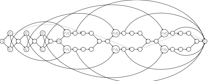
We summarize the complexity results of this section in Table 1.
[image:7.595.143.417.151.268.2]Interval Finite Axis-Parallel Ellipsoid General Ellipsoid Eval P(Thm. 1) P(Thm. 2) NPC(Thm. 3) NPC(Cor. 1) Solve Easy (Thm. 5) NPC(Thm. 4) Easy (Thm. 5) NPH(Thm. 6)
Table 1: Overview of the different complexity results of the minmax regret unconstrained combinatorial problem.
2.3
Shortest Path Problem
We assume in this section that U ⊂R+
n to avoid shortest path problems with
s
t
(28
Aa
1+ 3
a
1,
28
Aa
1−
a
1)
e
2(28
Aa
1,
4
Aa
1−
a
1)
e
3(28
Aa
n+ 3
a
n,
28
Aa
n−
a
n)
e
2n(28
Aa
n,
4
Aa
n−
a
n)
e
2n+1(
M, A
)
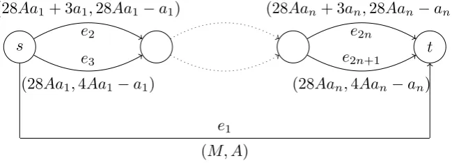
[image:8.595.132.457.256.373.2]e
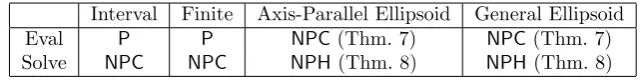
1Figure 1: The graph used in the proof of Theorem 7. The labels below and above each edge indicate the number of the edge and the values (ˆce, de) which
describe the uncertainty set.
finite uncertainty set withkscenarios, and only a single shortest path problem in the case of interval uncertainty.
We begin with the evaluation problem for ellipsoidal uncertainty sets in Theorem 7, before considering the solution problem in Theorem 8.
Theorem 7. The evaluation problem of (SP)for (axis-parallel) ellipsoidal
un-certainty sets isNP-complete.
Proof. We use again a reduction from the partition problem. For a given
in-stancea1, . . . , an we define the graph as shown in Figure 1.
The pairs (ˆce, de) on each edge define the size of the uncertainty set U =
{c: (c−ˆc)TD(c−cˆ)≤1}, where D is implicitly given by D−1
e :=de. M is a
sufficiently large constant depending on A. The set of all edges is denoted by
E0. The set of all edges except of the first edge is denoted by E =E0− {e1}.
Note that ˆce≥de ∀e∈E0 andde≥1∀e∈E0. Hence, U ⊂R+n. Consider the
problem of computing Reg(x) forx= (1,0, . . . ,0), i.e., the path consisting only of the first edgee1. Using Lemma 2 we can conclude that
Reg(x) = max
y∈Xmaxc∈U c
T(x−y)
= max
y∈X
ˆcT(x−y) + s
X
e∈E0
de(xe−ye)2
= ˆcTx−min
y∈X
ˆc
Ty−
s X
e∈E0
de(xe−ye)2
SinceM is a large constant we can exclude the solutiony= (1,0, . . . ,0) without changing the optimal value of the minimization problem. Further, we have that
y2k +y2k+1 = 1 ∀k = 1, . . . , n due to the structure of the graph. Hence, the
problem simplifies to
Reg(x) =M−min
y∈X
X
e∈E
ˆ
ceye−
s X
e∈E
deye+A
=M−min
y∈X
n X
k=1
y2k(28Aak+ 3ak) + (1−y2k)(28Aak)
− v u u t n X k=1
y2k(28Aak−ak) + (1−y2k)(4Aak−ak) +A !
=M−min
y∈X
28A
2+ 3
n X
k=1
y2kak−
v u u
t4A2+ 24A
n X
k=1
y2kak
Hence, the objective value of each solution y can be expressed by the value
λy= A1
Pn
k=1y2kak.
Reg(x) =M −min
y∈X
28A2+ 3Aλy− q
4A2+ 24A2λ
y
Consider the function f : [0,1] → R, f(λ) = 28A2+ 3Aλ− √
4A2+ 24A2λ.
The minimum of this function is attained for λ∗ = 0.5 due to the first order condition, further f(λ∗) = 28A2−2.5A. Hence,Reg(x)≥M−28A2+ 2.5Aif and only if the partition instance is a yes-instance.
Theorem 8. The solution problem of(SP)for (axis-parallel) ellipsoidal
uncer-tainty sets is NP-hard.
Proof. We use a reduction from exact 3-SAT which is known to beNP-complete.
We begin the construction by defining the uncertainty setU ={c: (c−cˆ)TD(c−
ˆ
c)≤1} with diagonal matrix D. We set the average cost of each edge e and the corresponding diagonal entry ofDto be 1, i.e., ˆce=Dee= 1∀e. Note that
U ⊂Rn+. Second, alls−tpaths consist ofLedges. With these restrictions the
minmax regret problem can be simplified as follows
min
x∈Xmaxc∈U
cTx−min
y∈Xc
Ty
= min
x∈Xmaxy∈X maxc∈U c
T(x−y)
= min
x∈Xmaxy∈X cˆ
T(x
−y) +||x−y||2
= min
x∈Xmaxy∈X (L−L+||x−y||2)
= min
x∈Xmaxy∈X
p
s l+
1
l− 1
l+ 2
l− 2
l+ 3
l− 3
C1
C1l+ 1
C1l− 1
C1l+ 2
C1l− 2
C1l+ 3
C1l− 3
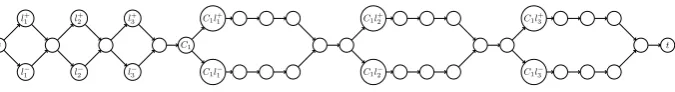
[image:10.595.129.467.123.169.2]t
Figure 2: This part of the graph (G1) is used to represent the literal and clause
assignments.
= min
x∈Xmaxy∈X
p
2L−2xTy
For each path represented by x denote by S(x) = miny∈XxTy the minimum
number of edges this path shares with all other s−t paths. Then, Reg(x) =
p
2L−2S(x). Therefore, minimizing the regret is equivalent to maximizing
S(x). For a given SAT instance, we construct a graph such that maxx∈XS(x)≥
1 if and only if the SAT instance is a yes-instance. This proves the theorem. Assume that we are given an instance of 3-SAT withnliteralsl1, . . . , ln and m clauses C1, . . . , Cm. To describe the graph we construct, we use a simple
example. Assume the 3-SAT instance contains only 3 literalsl1, l2, andl3 and
a single clause C1 = (l1∨l2∨l3). For clarity, we introduce the graph G in
three partsG1,G2, andG3. First we state the part of the graphG1 in Figure 2.
The next claims justify to restrict our attention toG1if we search for a pathx
maximizingS(x).
1. Claim: For all paths xin Git holds that S(x)≤1.
2. Claim: If a path xin Gexists withS(x) = 1, then there exists also a path
x0 contained inG1withS(x0) = 1.
The claims are proved at the end of the graph construction, when the com-plete graph is defined.
Each pathxinG1represents a literal and clause assignment. The first part
of the path from node s to node C1 represents the assignment of the literals.
For example: The assignment l1 = 0, l2 = 1, l3 = 1 is represented by the
path that contains the nodes l−1, l+2,andl+3. The second part of the path from node C1 to node t represents how the literals of clause C1 are chosen. If the
part contains for example the nodesC1l1+, C1l−2, andC1l+3, then we assign the
literals l1 = 1, l2 = 0, and l3 = 1 in clause C1. Note that all paths in this
graph have the same length. Two requirements need to be modeled. First, the assignment of the literals must correspond with the assignments of the literals in each clause and, second, the literal assignment should satisfy all clauses. In the next step we are going to introduce the part G2 and G3 which help to
model these requirements. The underlying idea is the following: If one of these two requirements is not fulfilled by the pathx, there exists another s−t path
y (containing edges of G2 or G3) which has no edge in common with x, i.e.,
S(x) = 0.
Next we introduce the partG2 which makes sure that the assignment of the
literals must be consistent with the assignments of the literals in each clause. We introduce chains of edges that connect the first part of G1 with the
second part ofG1as shown in Figure 3. Note that the length of each chain can
s l+
1
l− 1
l+ 2
l− 2
l+ 3
l− 3
C1
C1l+1
C1l−1
C1l+2
C1l−2
C1l+3
C1l−3
[image:11.595.127.468.149.284.2]t
Figure 3: The additional edges in the graph (G2) that model the relationship
betweenS(x) guarantee the consistency of literal assignment and literal assign-ment in each clause are thick. Each thick edge in the figure corresponds to a chain of edges in the graph.
pathxrepresents an inconsistent assignment forl1, e.g., letxcontain nodel+1
and C1l−1. We claim that in this case a path y exists withx
Ty = 0. Consider
the pathy that contains fromG1 only the nodess, l−1,C1l+1, the successor node
of C1l1+ and t. This path has no arc in common with x, hence, xTy = 0.
This relation holds analogously for the other literals l2 and l3. If only a single
inconsistent assignment is made, there exists a path y with xTy = 0. On the
other hand, if xrepresents a consistent assignment, all paths y in G1 and G2
have at least one edge in common with x.
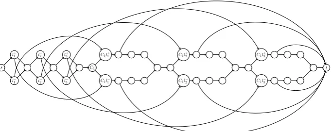
Next we introduce partG3 that models the relationship betweenS(x) and
the correct clause assignment. The additional chains of edges are shown in Figure 4. Again the length of each of these chains can be chosen in such a way that alls−tpaths have the same length.
Assume that clauseC1is not satisfied by the represented literal assignment,
i.e., path xcontainsC1l−1, C1l+2, andC1l−3. It is obvious that the pathy that
contains all three of the dotted chains has no edge in common withxand, hence,
S(x) = 0. Conversely, if only one literal is assigned such thatC1is fulfilled, this
path shares at least one arc withx.
We now show that if pathxrepresents a consistent literal and clause assign-ment, thenS(x)≥1, i.e., for every pathy it holds thatxTy≥1, if and only if
all clauses are fulfilled.
Assume thatxrepresents a literal assignment that fulfills all clauses. For the sake of contradiction assume that a path y exists that has no edge in common withx. It is an easy observation thaty contains either one of the thick or one of the dotted edges as, otherwise, it must contain the edge that leads to vertex
C1which is also contained inx. Ifycontains one dotted arc that leads to some
clause it must also contain the other dotted arcs that belong to this clause as
s l+
1
l− 1
l+ 2
l− 2
l+ 3
l− 3
C1
C1l+1
C1l−1
C1l+2
C1l−2
C1l+3
C1l−3
[image:12.595.125.470.150.285.2]t
Figure 4: The additional edges in the graph (G3) that model the relationship
betweenS(x) and the correct clause assignment are dotted. Each dotted edge in the figure corresponds to a chain of edges in the graph.
argument from above is valid. Ify contains one of the thick arcs this arc must correspond to a conflicting literal assignment (with respect to the assignment of
x), as every thick arc is connected to the contradicting assignment in the clause. The next edge of this path is contained inx, asxrepresents a consistent literal assignment.
On the other hand, ifxrepresents a literal assignment that violates at least one clause, there exists obviously a pathyusing the corresponding dotted edges withxTy= 0.
To conclude the proof, we have to show the two open claims.
Proof of Claim 1
Let xbe an arbitrary path inG. Observe that not both nodesl1+ and l1− can be contained inx. Without loss of generality letl1+ be not contained inx. We construct a path y which shares at most one edge with x. Denote by v the successor node ofC1l−1. Pathystarts with edge (s, l
+
1) next it uses the chain of
edges froml+1 toC1l1−and edge (C1l−1, v). Ifxcontains the chain of edges from
v to t, which are part of G2, we continue pathy by an arbitrary path from v
to tcontained inG1. In the other case, where the chain of edges fromv tot is
not contained inx, we continue pathysimply with this chain. The constructed pathy shares at most the edge (C1l1−, v) withx. This proves Claim 1.
Proof of Claim 2
Letxbe an arbitrary path inGwithS(x) = 1. We claim thatxmust fulfill the following properties: xmust contain nodeC1 and xmust contain at least one
of the nodesCil+k or Cil−k.
For the sake of contradiction assume first thatxdoes not contain C1. Then
there exists a pathy from stoC1 not sharing any edge withx. This path can
path from C1 to C1l+1 to t (using a chain of edges from G2) or the path from
C1 toC1l−1 tot (using a chain of edges fromG2) respectively.
For the sake of contradiction assume without loss of generality that C1l+1
and C1l−1 are not contained in x. Again we construct a pathy that shares no
edge with x. Without loss of generality assume thatl+1 is not contained inx. Path y starts with edge (s, l+1), followed by the chain of edges from G2 going
from l1+ to C1l−1, the edge (C1l−1, v) and the chain of edges fromG2 fromv to
t. Note thaty shares no edge withx.
Note that the first possible node a pathxfulfilling both of these properties can leaveG1 is at the third part of the last clause node. Denote byuthe last
node of xcontained inG1 (except fort). Note that there is only a single path
˜
xfromutotin G1. Consider the following pathx0. The first part fromstou
coincides withx. The second part is equal to ˜x. Note thatx0is contained inG
1
and shares edges with all pathsythat share edges withx. Hence,S(x0)≥S(x). This concludes the proof of Claim 2.
Note that the presented reduction uses a 3-SAT instance which consists of a single clause. The presented ideas generalize straightforward to the case of arbitrary 3-SAT instances. To introduce an additional literal ln, the first
part of the graph G1 is extended by l+n and ln−. The gadget representing an
additional clauseCm has exactly the same structure as the gadget forC1. The
corresponding gadget ofCmis put at the end of the graph.
Note that Theorem 8 even holds for (SP) instances where all edges have the same cost structure, the uncertainty set is a perfect ball and alls−tpaths contain the same number of edges. The same construction can be used to show that the minmax regret shortest path problem isNP-complete even if the costs of all edges belong to [0,1]. This is a refinement of the original complexity proof of Averbakh and Lebedev [AL04], where two types of intervals ([0,1] and [1,1]) are used.
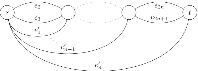
The complexity results of this section are summarized in Table 2
[image:13.595.135.457.503.543.2]Interval Finite Axis-Parallel Ellipsoid General Ellipsoid Eval P P NPC(Thm. 7) NPC(Thm. 7) Solve NPC NPC NPH(Thm. 8) NPH(Thm. 8)
Table 2: Overview of the different complexity results of the minmax regret shortest path problem.
2.4
Spanning Tree Problem
In this section we sketch how to transfer results on the minmax regret shortest path problem to the minmax regret minimum spanning tree problem.
Very similar to the case of the minmax shortest path problem the minmax regret minimum spanning tree problem is well-researched for interval and finite uncertainty sets. For a finite, but constant number of scenarios, the problem is
s
t
. .
.
e
2e
3e
2ne
2n+1e
01e
0n−1 [image:14.595.125.466.131.254.2]e
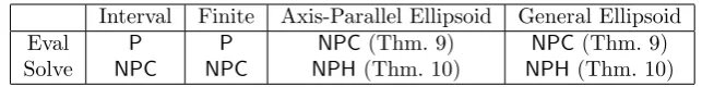
0nFigure 5: The graph used in the proof of Theorem 9.
Theorem 9. The evaluation problem of (M ST) for (axis-parallel) ellipsoidal
uncertainty sets is NP-complete.
Proof. We only give a sketch of the proof, since it is essentially the same as
the proof of Theorem 7. Using the same notation, we define a reduction from the partition problem again. The constructed graph is almost the undirected version of the graph defined in Figure 1. Instead of edge e1 that represented
a path for which we computed the regret, we define a set of edges {e01, . . . , e0n}
that form a spanning tree. The cost structure of the edgese2, . . . , e2n+1 is the
same as given in Figure 1. The costs of the edgese01, . . . , e0n are M,An
. Denote by x the spanning tree that consists of e01, . . . , e0n. The goal is to
evaluate Reg(x). By searching for the spanning tree that defines Reg(x) we can exclude all spanning trees that contain an edgee0i due to the large nominal cost. Note that all remaining spanning trees form s−t paths. Hence, the problem of computingReg(x) is analogous to the problem defined in the proof of Theorem 7.
Theorem 10. The solution problem of (M ST) for (axis-parallel) ellipsoidal
uncertainty sets is NP-hard.
Proof. Note that each spanning tree containsn−1 edges. Hence, by defining the
same cost structure as in the proof of Theorem 8 we derive an equivalent relation. For an arbitrary spanning tree x we obtain that Reg(x) = p2n−2−S(x). Here, S(x) denotes the minimal number of edges each other spanning tree has in common withx. Hence, minimizingReg(x) is equivalent to maximizingS(x). In [AL04] it is shown that maximizingS(x) isNP-complete.
Summarizing these results we obtain the same table as for the shortest path problem (see Table 2).
3
Solution Approaches
Interval Finite Axis-Parallel Ellipsoid General Ellipsoid Eval P P NPC(Thm. 9) NPC(Thm. 9) Solve NPC NPC NPH(Thm. 10) NPH(Thm. 10)
Table 3: Overview of the different complexity results of the minmax regret minimum spanning tree problem.
relaxation procedure for interval uncertainty in Section 3.1, before introducing exact solution approaches for ellipsoidal sets in Section 3.2.
3.1
Scenario Relaxation for Interval Sets
For combinatorial minmax regret problems with interval uncertainty sets, one of the most frequently used solution method is to generate a finite set of scenarios iteratively (see [ABV09]). There are (at least) two ways to do so. We briefly explain them in the following.
A general minmax regret problem of the form
min
x∈Xmaxc∈U c
Tx−opt(c)
can be rewritten as:
minz
s.t. z≥cTx−cTy ∀c∈ U, y∈ X
x∈ X
In case of an interval uncertainty set, these are infinitely many constraints. Even restricting ourselves to extreme points of the uncertainty set, there are still exponentially many. For this reason, we generate them iteratively during the solution process.
Let us consider the constraints
z≥cTx−cTy ∀y∈ X ∀c∈ U
withU =
×
i∈[n][ci, ci]. If we fix somec∈ U, we can read this asz≥max
y∈X c
Tx−cTy
which is equivalent to
z≥cTx−opt(c). (4)
That is, we can iteratively generate scenarios c∈ U and add constraints of the form (4) to solve the robust problem. To find the nextc ∈ U in each iteration (that is, a maximizer of the right-hand side of (4)), one simply usesc∗(x), with
c∗(x)i :=ci+ (ci−ci)xi (see [ABV09] for a proof of this statement). To find opt(c∗(x)), a problem of the nominal type needs to be solved. We refer to constraints of this kind as type 1 cuts.
Analogously, we can consider constraints of the form
That is, for fixedy∈ X, let us consider
z≥max
c∈U c
Tx−cTy
in more detail. This is equivalent to setting
z≥c∗(x)Tx−c∗(x)Ty. (5)
It is then possible to rewritec∗(x) such that this becomes a linear integer pro-gram. We refer to constraints of this kind as type 2 cuts. To find the next such cut, we need to solve a nominal problem withc∗(x), just like for type 1.
Note that type 2 cuts are more ”flexible” in the sense that they only fix a solution y, and use the worst-case scenario depending onx. For type 1 cuts, both scenarioc and solutiony are fixed. For this reason, it can be shown that type 2 cuts are more efficient (tighter) than type 1 cuts [ABV09].
3.2
Solution Approaches for Ellipsoidal Sets
We now consider minmax regret problems with general ellipsoidal uncertainty setsU ={cˆ+Cξ:kξk2≤1}. Also in this case, we have constraints of the form
z≥cTx−cTy ∀c∈ U, y∈ X
that need to be reformulated to solve the problem. We consider two ways to do so. First, let us fixc∈ U. Then, just as for interval uncertainty, the constraints become equivalent to
z≥max
y∈X c
Tx
−cTy
⇐⇒ z≥cTx−opt(c).
However, generating the next such constraint for a givenx∈ X is more complex. We need to solve the problem of finding the largest such cut, that is,
max
c∈U c
Tx−opt(c)
.
This is equivalent to:
maxcTx−cTy
s.t. c= ˆc+Cξ
kξk2≤1
y∈ X
Using Lemma 1, we find that this problem is equivalent to
max ˆcT(x−y) +z
s.t. z2≤ kCT(x−y)k22 (SUB)
y∈ X, z≥0.
To solve problem (SUB), we consider two linearizations of the right-hand side. In our first approach, we use thatxi=x2i for binary variablesxi and find that
kCT(x−y)k2 2=
X
i∈[n]
X
j∈[n]
C
2
ji(xj−2xjyj+yj) + X
k<j
2CjiCki(xj−yj)(xk−yk)
To linearize products of the formyjyk, we introduce new binary variablesαjk
with
yj+yk≤1 +αjk and 2αjk≤yj+yk.
Using this linearization of the right-hand side in (SUB), we arrive at a convex quadratic integer program.
As a second approach, we rewrite the constraint as
kCT(x−y)k2 2=v
TQv= X
i∈[n]
viai(v)
withvi:=xi−yi,Q:=CCT andaj(v) := (Qv)j =Pi∈[n]qjivi. We introduce
new variableshj :=vjaj(v) and linearize them using the following constraints.
For anyj∈[n] withvj ∈ {0,1}(i.e.,xj= 1) we set
hj ≤
X
i∈[n]
qjivi+Mj−(1−vj) and hj ≤Mj+vj.
For anyj∈[n] withvj ∈ {−1,0} (i.e.,xj = 0), we use instead
hj ≤ −
X
i∈[n]
qjivi+Mj+(1 +vj) and hj≤ −Mj−vj.
The constants Mj+ and Mj− are chosen such that Mj+ ≥ maxvPi∈[n]qjivi
and Mij− ≥ −minvPi∈[n]qjivi. To this end, we set Mj+ := P
i∈[n]qjixi and
Mj− :=P
i∈[n]qji(1−xi) as the smallest possible such constants.
Note that the second linearization requires less additional variables (linearly instead of quadratically many), but is numerically less stable due to the ”big-M” constraints.
Solving (SUB) we findy∗, and the correspondingc∗is given by ˆc+Cξ∗ with
ξ∗=CT(x−y∗)/kCT(x−y∗)k
2.
As for interval uncertainty sets, we refer to this procedure as type 1 cuts.
For the second type of cuts, we fix y ∈ X, in which case our constraints become
z≥cTx−cTy ∀c∈ U
which is a ”classic” robust optimization constraint, i.e., using Lemma 1 it can be reformulated to
z≥ˆcT(x−y) +kCT(x−y)k2.
This is again a conic quadratic constraint. To generate new cuts of this form, we maximize the right-hand-side iny, which is the same subproblem as described in (SUB).
To summarize, both approaches need to solve the same subproblem to gener-ate new cuts. Using cuts of type 1 amounts to master problems that are integer linear, while cuts of type 2 amount to master problems that are second order cone integer. In principle, master problems for type 2 are therefore harder to solve. However, they have the advantage that they give a tighter formulation.
Proof. Let some x ∈ X be fixed, and let c and y be generated from the sub-problem (SUB). Then we have
cTx−opt(c) =cTx−cTy
≤max
c0∈U
c0Tx−c0Ty= ˆcT(x−y) +kCT(x−y)k2
We conclude this section by considering an approximation algorithm. As one can easily see,U is symmetric with respect to ˆc. Using Property 3.3 from [Con12], we get the following result.
Theorem 12. The midpoint solution
ˆ
x∈arg min{cˆTx:x∈ X }
is a 2-approximation for the minmax regret problem with ellipsoidal uncertainty set.
4
Computational Experiments
The purpose of these experiments it to compare the performance of type 1 and type 2 cuts for general ellipsoidal uncertainty sets, using one of the two linearizations for problem (SUB). To this end, we use both unconstrained and shortest path problems as a testbed.
4.1
Setup
We generate uncertain unconstrained problems of the form
mincTx:x∈ {0,1}n
by creating random ellipsoidal uncertainty sets U. For all instances, we gener-ate ˆci ∈ {−100, . . . ,100} and Cii ∈ {50, . . . ,150}. Additionally, non-diagonal
entries ofC are generated in three different ways:
• Sets with small deviation, whereCij∈ {1, . . . ,50}
• Sets with medium deviation, whereCij ∈ {1, . . . ,50} with a probability
of 75%, and inCij ∈ {50, . . . ,200} with 25%.
• Sets with large deviation, whereCij ∈ {50, . . . ,200}.
Parameters were always generated uniformly at random from the respective sets of possible outcomes. Each non-diagonal entry is generated with a certain probabilityp∈ {5%,15%,25%}. For each number of itemsninN ={10+20N :
N ∈ {0, . . . ,7}} we therefore generated nine instance sets, which which we
denote as Ip,y
n with n items and y ∈ {s, m, l} for small, medium, and large
deviation, respectively. We abbreviate Is, Im, Il and I5, I15, I25 to denote
all instances of the respective type (i.e.,Im denotes all instances with medium
with 5% probability). For each instance set, we generated 10 instances, which means a total of 720 instances were considered.
Additionally, we generated a second set of test instances for shortest path problems. All parameters are chosen in the same way as for the unconstrained problems. The graphs we consider are layered graphs with 4 nodes per layer, andnlayers withn∈ {2, . . . ,9}. Between two layers, all possible forward edges were generated. We denote these instances asJp,y
n , with the same abbreviations
as for I. For each instance set, 10 instances were generated (720 instances in total).
We use the two scenario relaxation procedures described in Section 3. In the following, we denote the solution approach that uses type 1 cuts of the form
z≥cTx−opt(c)
as C1, and the approach based on type 2 cuts of the form
z≥ˆcT(x−y) +kCT(x−y)k2
as C2. Recall that C1 generates master problems that are likely to be easier to solve, while C2 has tighter bounds and might need less iterations. Depending on how the subproblem (SUB) is linearized, we append either ”-A” (for the first linearization with quadratically many variables) or ”-B” (for the second linearization with linearly many variables) to the name of the method.
We used CPLEX v.12.6 [IBM13] to solve all linear and quadratic integer programs on a computer with a 16-core Intel Xeon E5-2670 processor, running at 2.60 GHz with 20MB cache, and Ubuntu 12.04. Processes were pinned to one core. A time limit of 900 seconds was used per method and instance.
4.2
Experiment 1: Unconstrained Problems
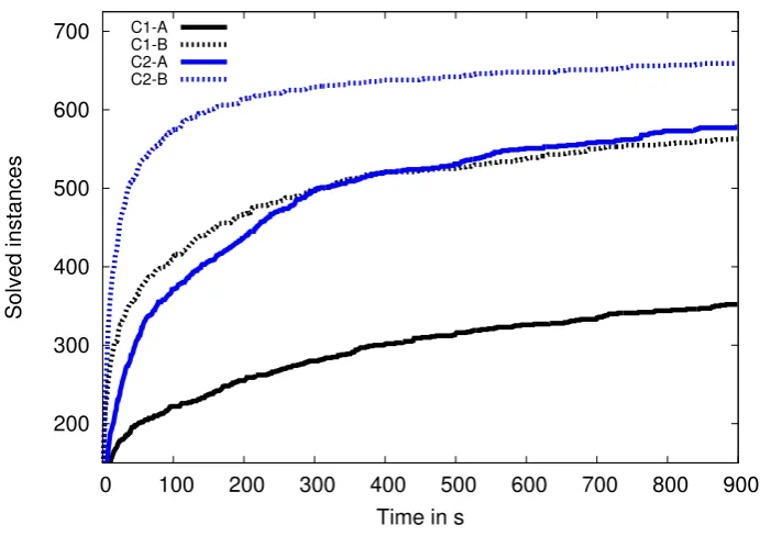
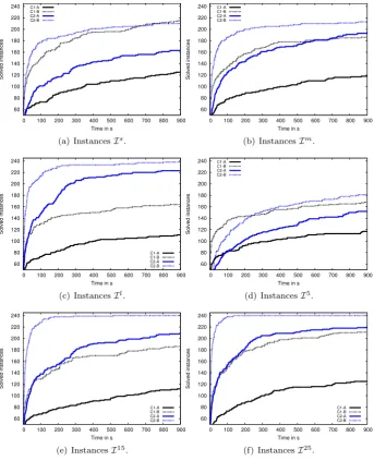
Figure 6 shows the resulting performance profile over all 720 unconstrained instances, i.e., at every time step, we plot how many instances have been solved to optimality. Plotted in black is C1, while C2 is in blue. Method A linearization of sub is a full line, and method B linearization is a dashed line. In Figure 7, the performance is shown over different instance classes.
The results indicate that method B clearly outperforms method A to solve subproblems. As C1 requires more cuts (and therefore the subproblem is solved more often), using the better method gives an even larger performance im-provement than for C2. However, method B is numerically less stable due to the bigM constants, which are particularly large when the matrix C is dense. For five instances, the subproblem could not be solved by Cplex due to numeri-cal instability, which we counted as if the time limit of 900 seconds was reached for the purpose of this evaluation.
200 300 400 500 600 700
0 100 200 300 400 500 600 700 800 900
Solved instances
Time in s C1-A
[image:20.595.123.469.121.365.2]C1-B C2-A C2-B
Figure 6: Performance profile for unconstrained problems, all instances.
Overall, solution approach C2-B shows the best performance to solve the minmax regret problem with ellipsoidal uncertainty on the instances we consid-ered here.
4.3
Experiment 2: Shortest Path Problems
We now consider the performance of our algorithms on shortest path instances. In Figure 8, we present performance profile over all 720 instances, and a more differentiated view on instance classes in Figure 9.
In this case, the strong performance of C2 for high-density matricesC with large values that could be observed for unconstrained instances cannot be ob-served. The reason for this is that it does not suffice to generate the two cuts
y = 0 and y = 1, as these are infeasible in this setting. Hence, performance of C2 actually deteriorates if the density of C or the size of the values in C
increase.
The relative order of the methods, i.e., subproblems B perform better than A and cuts of type 2 perform better than cuts of type 1 is the same as before. Hence, also for these shortest path problems, we find that the best solution approach is given by C2-B. More detailed tables are given in Appendix A.
5
Conclusion
60 80 100 120 140 160 180 200 220 240
0 100 200 300 400 500 600 700 800 900
Solved instances
Time in s C1-A
C1-B C2-A C2-B
(a) InstancesIs.
60 80 100 120 140 160 180 200 220 240
0 100 200 300 400 500 600 700 800 900
Solved instances
Time in s C1-A
C1-B C2-A C2-B
(b) InstancesIm.
60 80 100 120 140 160 180 200 220 240
0 100 200 300 400 500 600 700 800 900
Solved instances
Time in s
C1-A C1-B C2-A C2-B
(c) InstancesIl.
60 80 100 120 140 160 180 200 220 240
0 100 200 300 400 500 600 700 800 900
Solved instances
Time in s C1-A
C1-B C2-A C2-B
(d) InstancesI5.
60 80 100 120 140 160 180 200 220 240
0 100 200 300 400 500 600 700 800 900
Solved instances
Time in s
C1-A C1-B C2-A C2-B
(e) InstancesI15.
60 80 100 120 140 160 180 200 220 240
0 100 200 300 400 500 600 700 800 900
Solved instances
Time in s
C1-A C1-B C2-A C2-B
[image:21.595.126.470.203.627.2](f) InstancesI25.
200 300 400 500 600 700
0 100 200 300 400 500 600 700 800 900
Solved instances
Time in s
[image:22.595.122.468.120.364.2]C1-A C1-B C2-A C2-B
Figure 8: Performance profile for shortest path problems, all instances.
this work, we considered minmax regret problems with ellipsoidal uncertainty sets.
We gave a thorough discussion of arising problem complexities for the un-constrained combinatorial problem, and the shortest path problem. To solve these problems, two types of cuts that can be used in a scenario relaxation pro-cedure were derived, as well as two linearizations to solve the subproblem of generating new cuts. We compared the performance of these methods in two computational experiments, using unconstrained and shortest path problems as a testbed.
We found that the increased complexity of master problems with type 2 cuts are worth the effort, as less iterations are required to solve the minmax regret problem to optimality. The advantage is particularly strong for the un-constrained problem if the values of the deviation matrixCare dense and large. In future research, heuristic solution algorithms should be developed and tested, due to the high computational effort when solving these problems.
References
[ABV05] H. Aissi, C. Bazgan, and D. Vanderpooten. Complexity of the min–max and min–max regret assignment problems.
Opera-tions Research Letters, 33(6):634–640, 2005.
[ABV07] H. Aissi, C. Bazgan, and D. Vanderpooten. Approximation of min–max and min–max regret versions of some combinato-rial optimization problems. European Journal of Operational
60 80 100 120 140 160 180 200 220 240
0 100 200 300 400 500 600 700 800 900
Solved instances
Time in s
C1-A C1-B C2-A C2-B
(a) InstancesJs.
60 80 100 120 140 160 180 200 220 240
0 100 200 300 400 500 600 700 800 900
Solved instances
Time in s
C1-A C1-B C2-A C2-B
(b) InstancesJm.
60 80 100 120 140 160 180 200 220 240
0 100 200 300 400 500 600 700 800 900
Solved instances
Time in s C1-A
C1-B C2-A C2-B
(c) InstancesJl.
60 80 100 120 140 160 180 200 220 240
0 100 200 300 400 500 600 700 800 900
Solved instances
Time in s
C1-A C1-B C2-A C2-B
(d) InstancesJ5.
60 80 100 120 140 160 180 200 220 240
0 100 200 300 400 500 600 700 800 900
Solved instances
Time in s
C1-A C1-B C2-A C2-B
(e) InstancesJ15.
60 80 100 120 140 160 180 200 220 240
0 100 200 300 400 500 600 700 800 900
Solved instances
Time in s C1-A
C1-B C2-A C2-B
[image:23.595.124.470.203.625.2](f) InstancesJ25.
[ABV09] H. Aissi, C. Bazgan, and D. Vanderpooten. Min–max and min–max regret versions of combinatorial optimization prob-lems: A survey. European Journal of Operational Research, 197(2):427–438, 2009.
[AL04] I. Averbakh and V. Lebedev. Interval data minmax regret network optimization problems.Discrete Applied Mathematics, 138(3):289–301, 2004.
[AL05] I. Averbakh and V. Lebedev. On the complexity of minmax regret linear programming. European Journal of Operational
Research, 160(1):227–231, 2005.
[Ave01] I. Averbakh. On the complexity of a class of combinatorial optimization problems with uncertainty. Mathematical
Pro-gramming, 90(2):263–272, 2001.
[BBC11] D. Bertsimas, D. Brown, and C. Caramanis. Theory and appli-cations of robust optimization. SIAM Review, 53(3):464–501, 2011.
[BBI14] F. Baumann, C. Buchheim, and A. Ilyina. A Lagrangean de-composition approach for robust combinatorial optimization. Technical report, Optimization Online, 2014.
[BS04] D. Bertsimas and M. Sim. The price of robustness.Operations
Research, 52(1):35–53, 2004.
[BTGN09] A. Ben-Tal, L. El Ghaoui, and A. Nemirovski. Robust
Opti-mization. Princeton University Press, 2009.
[BTN98] A. Ben-Tal and A. Nemirovski. Robust convex optimization.
Mathematics of Operations Research, 23(4):769–805, 1998.
[BTN99] A. Ben-Tal and A. Nemirovski. Robust solutions of uncer-tain linear programs. Operations Research Letters, 25(1):1–13, 1999.
[CG15] A. Chassein and M. Goerigk. A new bound for the midpoint solution in minmax regret optimization with an application to the robust shortest path problem. European Journal of
Oper-ational Research, 244(3):739–747, 2015.
[CG16] A. Chassein and M. Goerigk. Performance analysis in robust optimization. InRobustness Analysis in Decision Aiding,
Op-timization and Analytics, chapter 7. Springer, 2016.
[Con12] E. Conde. On a constant factor approximation for minmax regret problems using a symmetry point scenario. European
Journal of Operational Research, 219(2):452–457, 2012.
[GS16] M. Goerigk and A. Sch¨obel. Algorithm engineering in robust optimization.Algorithm and Engineering: Selected Results and
[IBM13] IBM. IBM ILOG CPLEX 12.6 User’s Manual, 2013.
[IS95] M. Inuiguchi and M. Sakawa. Minimax regret solution to linear programming problems with an interval objective function.
Eu-ropean Journal of Operational Research, 86(3):526–536, 1995.
[KY97] P. Kouvelis and G. Yu. Robust Discrete Optimization and Its
Applications. Springer Science & Business Media, 1997.
[KZ06] A. Kasperski and P. Zieli´nski. An approximation algorithm for interval data minmax regret combinatorial optimization prob-lems. Information Processing Letters, 97(5):177–180, 2006.
[MGD04] R. Montemanni, L. M. Gambardella, and A. V. Donati. A branch and bound algorithm for the robust shortest path prob-lem with interval data.Operations Research Letters, 32(3):225– 232, 2004.
[PGAMCVT14] F. P´erez-Galarce, E. ´Alvarez-Miranda, A. Candia-V´ejar, and P. Toth. On exact solutions for the minmax regret spanning tree problem.Computers and Operations Research, 47(0):114– 122, 2014.
[TTT10] A. Takeda, S. Taguchi, and T. Tanaka. A relaxation algorithm with a probabilistic guarantee for robust deviation optimiza-tion. Computational Optimization and Applications, 47(1):1– 31, 2010.
[YY98] Gang Yu and Jian Yang. On the robust shortest path problem.
A
Appendix
We present detailed results for the experiments described in Section 4. In Ta-bles 4 and 6, we show the average number of cuts and the number of problems that were solved to optimality for each instance set. We show how much time was spent in the relaxed master problem and in the subproblem in Tables 5 and 7.
C1-A C1-B C2-A C2-B
Inst. Cuts Opt Cuts Opt Cuts Opt Cuts Opt
I5
s 57.0 45 160.1 65 12.7 43 13.6 50
I15
s 18.5 38 48.6 72 3.6 60 3.9 80
I25
s 9.2 41 19.3 77 2.7 59 2.9 79
I5
m 33.2 39 142.9 53 9.0 46 10.2 53
I15
m 20.5 35 75.5 57 3.7 68 3.7 79
I25
m 21.5 43 53.7 75 2.5 79 2.5 80
I5
l 26.6 32 136.3 49 5.0 62 5.5 77
I15
l 25.4 38 92.9 56 2.3 80 2.3 80
I25
[image:26.595.164.431.216.371.2]l 32.7 40 77.4 58 2.0 80 2.0 80
Table 4: Results for unconstrained instances. ”Cuts” is the average number of cuts that were generated during the solution process. ”Opt” is the number of problems that were solved to optimality, out of 80 for each instance type.
C1-A C1-B C2-A C2-B
Inst. Main SUB Main SUB Main SUB Main SUB
I5
s 5.8 94.2 55.8 44.2 73.5 26.5 97.8 2.2
I15
s 2.0 98.0 8.8 91.2 21.6 78.4 65.7 34.3
I25
s 1.3 98.7 5.0 95.0 12.6 87.4 43.6 56.4
I5
m 4.0 96.0 48.5 51.5 60.6 39.4 95.4 4.6
I15
m 2.7 97.3 16.8 83.2 25.2 74.8 73.0 27.0
I25
m 2.5 97.5 17.3 82.7 18.6 81.4 70.4 29.6
I5
l 3.2 96.8 45.9 54.1 37.9 62.1 93.1 6.9
I15
l 2.2 97.8 46.4 53.6 24.5 75.5 86.0 14.0
I25
l 4.6 95.4 64.1 35.9 27.5 72.5 90.8 9.2
[image:26.595.155.439.438.591.2]C1-A C1-B C2-A C2-B
Inst. Cuts Opt Cuts Opt Cuts Opt Cuts Opt
J5
s 11.4 69 13.2 80 2.6 79 2.6 80
J15
s 10.0 59 17.0 80 2.4 65 2.6 80
J25
s 8.9 46 19.7 79 2.1 59 2.7 80
J5
m 15.1 62 21.0 80 2.8 80 2.8 80
J15
m 15.2 45 43.1 78 3.0 60 3.8 80
J25
m 12.4 31 63.2 63 2.6 50 4.0 80
J5
l 24.0 45 57.2 79 3.7 76 3.8 80
J15
l 15.9 29 80.1 54 2.7 44 4.9 74
J25
[image:27.595.165.430.171.328.2]l 14.7 20 79.8 48 2.8 39 5.2 66
Table 6: Results for shortest path instances. ”Cuts” is the average number of cuts that were generated during the solution process. ”Opt” is the number of problems that were solved to optimality, out of 80 for each instance type..
C1-A C1-B C2-A C2-B
Inst. Main SUB Main SUB Main SUB Main SUB
J5
s 0.8 99.2 17.4 82.6 23.6 76.4 83.1 16.9
J15
s 0.8 99.2 2.5 97.5 22.4 77.6 57.7 42.3
J25
s 0.7 99.3 1.9 98.1 17.3 82.7 50.6 49.4
J5
m 0.7 99.3 11.5 88.5 32.1 67.9 85.3 14.7
J15
m 1.1 98.9 4.9 95.1 34.2 65.8 80.9 19.1
J25
m 0.9 99.1 5.4 94.6 27.7 72.3 82.2 17.8
J5
l 1.4 98.6 9.2 90.8 44.0 56.0 86.6 13.4
J15
l 1.3 98.7 9.3 90.7 27.6 72.4 87.4 12.6
I25
l 0.8 99.2 9.6 90.4 19.0 81.0 78.0 22.0
[image:27.595.155.439.474.627.2]