Preferences and social influence

warwick.ac.uk/lib-publications

Freshman, Chaim and Segal, Uzi. (2017) Preferences and social influence. American Economic Journal : Microeconomics.

Permanent WRAP URL:

http://wrap.warwick.ac.uk/91992

Copyright and reuse:

The Warwick Research Archive Portal (WRAP) makes this work by researchers of the University of Warwick available open access under the following conditions. Copyright © and all moral rights to the version of the paper presented here belong to the individual author(s) and/or other copyright owners. To the extent reasonable and practicable the material made available in WRAP has been checked for eligibility before being made available.

Copies of full items can be used for personal research or study, educational, or not-for-profit purposes without prior permission or charge. Provided that the authors, title and full

bibliographic details are credited, a hyperlink and/or URL is given for the original metadata page and the content is not changed in any way.

Publisher’s statement:

Permission to make digital or hard copies of part or all of American Economic Association publications for personal or classroom use is granted without fee provided that copies are not distributed for profit or direct commercial advantage and that copies show this notice on the first page or initial screen of a display along with the full citation, including the name of the author. Copyrights for components of this work owned by others than AEA must be honored. Abstracting with credit is permitted.

The author has the right to republish, post on servers, redistribute to lists and use any component of this work in other works. For others to do so requires prior specific permission and/or a fee. Permissions may be requested from the American Economic Association Administrative Office by going to the Contact Us form and choosing "Copyright/Permissions Request" from the menu.

Copyright © 2017 AEA

A note on versions:

The version presented here may differ from the published version or, version of record, if you wish to cite this item you are advised to consult the publisher’s version. Please see the ‘permanent WRAP URL’ above for details on accessing the published version and note that access may require a subscription.

Preferences and Social Influence

Chaim Fershtman

Uzi Segal

August 21, 2017

Abstract

Interaction between decision makers may affect their preferences. We consider a setup in which each individual is characterized by two sets of preferences: his unchanged core preferences and his behavioral preferences. Each individual has a social influence function that de-termines his behavioral preferences given his core preferences and the behavioral preferences of other individuals in his group. Decisions are made according to behavioral preferences. The paper considers dif-ferent properties of these social influence functions and their effect on equilibrium behavior.

Keywords: Risk aversion, social influence, behavioral preferences.

1

Introduction

Consider a person sitting by himself in an empty restaurant, looking over the menu in order to decide what to order. Now consider a slightly different scenario in which the same person is sitting to a long table together with other people, each of them in the process of ordering their meals. They may

∗_{We would like to thank the editor, Andy Postlewaite, and two anonymous referees for} many valuable comments. We also thank Sushil Bikhchandani, Kim Border, Edi Karni, and Joel Sobel for their comments and help, and Zhu Zhu of Boston College for helpful research assistance.

comment about their preferences, but as they don’t have any information about the dishes they do not make remarks regarding the menu.1 _{Do we}

expect the diner to order the same dish? Standard analysis seems to suggest that the choice should be the same in both situations and that each individual will choose the dish that he likes best. Yet, Ariely and Levav [1] provide a convincing experiment that suggests that this is not the case and that the presence of a group (even of complete strangers) affects the choice of meals. Specifically, they found a larger variance in the dishes ordered by individuals that were part of a group than by individuals that were sitting by themselves. The group effect on preferences and attitudes has been extensively dis-cussed in social psychology. One of the well-documented effects is the phe-nomenon of group polarization, where group interactions make group mem-bers more extreme than their initial inclination. For example, Myers [26] reports the effect of group discussion on women with moderately feminist views, that following a group interaction demonstrate stronger feminist views. Focusing on attitude towards risky choices, Aronson [2, p. 273] claims that group discussions may make people more risk taking than their initial ten-dencies. It is also claimed that established groups exhibit less polarization than new groups of people that do not know each other, where more profound polarization is demonstrated (see Myers and Lamm [27]).

Consider two possible situations for a decision maker who is trying to decide whether to accept or reject a lottery. In the first, he is making his decision in isolation, while in the second scenario he is part of a group of individuals, all of them facing a similar problem. Moreover, assume that the lottery determines only the decision maker’s individual payoffs and does not affect the well-being of anyone else. Assume further that all choices are observable. Will the different environments lead to different decisions? Following the restaurant example we assume they do, and our aim is to investigate the structure and consequences of these influences.

We assume that each individual is characterized by two sets of preferences: his true core preferences and his behavioral preferences, where actual choice is determined by the behavioral preferences. These latter preferences are observable by all other players and each player has a group influence function that determines his behavioral preferences as a function of his core preferences and the observed behavioral preferences of other individuals. Clearly, if he

1

is not influenced by others, then his behavioral preferences are the same as his core preferences. We do not assume a model of preferences evolution, as individuals’ core preferences do not change as a result of social interaction. Rather, individuals change their behavior in different social environments given the behavioral preferences of other individuals in their relevant social group. When a person moves to a different social environment he may change his behavior, which is now the outcome of the same core preferences and a different profile of other people’s behavioral preferences. We emphasize that our interpretation of the social influence function is of interaction, and not of aggregation. That is, an individual is influenced by (and influences) others’ behavior, but he does not try to behave as a social planner by taking an average (or another combination) of his and other people’s preferences. Moreover, even if he is aware of the fact that other decision makers are influenced by his behavior, he does not behave strategically.

We discuss conditions on the social influence functions that guarantee the existence of such an equilibrium of interdependent behavioral preferences. We investigate properties of the social influence function which induce simple adjustments. In particular, we offer conditions under which the core utility of person i is transformed by a function hi that depends on the average

behavioral utilities of everyone else. According to our analysis, the social influence does not necessarily imply regression to the mean. It may, for example, induce all group members to behave as if they are all more (or all less) risk averse than they really are according to their core preferences.

action chosen by an individual affects directly his social status (for example, attending college) or it affects the perceptions about his type which deter-mines his status (e.g., driving a Porsche). As an exception to this approach, see Cole, Mailath, and Postlewaite [11], where incentives to get a higher sta-tus do not enter directly into the utility but affect the probability of getting a good matching. When actions signal individuals’ type and social status is an important concern, Bernheim’s individuals converge to a conformist be-havior. In other cases individuals would like to choose a product that other people do not choose simply because they want to be fashionable or different (see for example Karni and Schmeidler [23]).

Our framework is closely related to Postlewaite [30] (see also Mailath and Postlewaite [25] and Postlewaite [29]), where two types of preferences are con-sidered. “Deep preferences,” which capture the immediate satisfaction, and “reduced form preferences,” which take into account future consequences. Thus the reduced form preferences capture the fact that preferences over goods and services are not exogenous but they are in fact endogenous social constructions that may be affected by the consumption habits of other people in the group. In particular, with this setup it is possible to discuss the effect of social norms on behavior and the observation that there is a substantial differences in behavior among social groups even when their deep preferences are identical. Our setting focuses on social influence in small groups in which individuals observe the behavior of other individuals in the group. Our core preferences may capture any immediate satisfaction as well as future social consequence, and in particular different types of social norms. Moreover the type of social interaction that we consider does not necessarily have any fu-ture social consequences and yet it affects behavior. A possible fusion of the two settings is a framework with three types of preferences: the deep pref-erences, the reduced form preferences that capture all the social norms and social consequences of behavior in a society, and the behavioral preferences that governs daily decision which depend on frequent interaction in different social groups in which the observed daily decisions of individuals interact with one another.

taken by other people. By assuming such interdependent preferences the literature focuses for example on altruism, fairness concerns, reciprocity, or inequality aversion.2 _{We do not wish to put restrictions on the nature of}

individual preferences and they may be purely egoistic or socially benevolent. That is, in our setting individuals may have preferences that are defined only with respect to their own payoffs or they may have social preferences. But what we assume is that when these individuals need to make decisions their preferences may be affected by the preferences of other individuals even when those individuals have no direct economic or strategic interaction with the decision makers. For example, the decision maker’s degree of risk aversion or level of altruism may be influenced by other people’s attitude to risk or altruism.

Our setting focuses on the formation of endogenous behavioral prefer-ences that are subject to social influence. There is an extensive literature on preferences formation and on endogenous preferences. One approach, which is based on evolutionary sociobiology (see Becker [3], Dawkins [13], and Frank [20]), assumes that people are influenced by “successful” individ-uals and that they eventually adopt their preferences. For an overview of this literature, see Samuelson [31]. In this approach, the meaning of “successful” is exogenously given and typically takes the form of higher monetary pay-offs. The second approach for endogenous preferences is the dynamic cultural transmission framework (see Bisin and Verdier [5], Boyd and Richardson [7], and Cavalli-Sforza and Feldman [8]). This setting assumes a two stage so-cialization process. The first is a direct soso-cialization, where parents try to teach their children to adopt their own cultural identity. Whenever direct so-cialization fails, children adopt the cultural identity of a random role model. In our approach we assume that individuals are influenced by all members of their social group regardless of their relative success, a concept which may be meaningless, for example, when choosing a meal. Our approach there-fore captures social influence without introducing any strategic, altruistic, or evolutionary purpose for such an influence.

The paper is organized as follows. In section 2 we set up our model of social influence functions and establish the existence of equilibrium of behavioral preferences. In section 3 we consider different properties of social

2

influence functions and of behavioral preferences. Section 4 presents a simple environment in which preferences are represented by a single parameter (like risk aversion) and shows under what conditions social influence makes players become more or less extreme. Section 5 provides some concluding comments.

2

Preliminaries

We assume n individuals. Each person i has two continuous vNM utility functions on outcomes in [a, b]: The first utility, ui, represents his core

pref-erences. The second, vi, represents his behavioral preferences. Since vNM

functions are unique up to positive affine transformations, we assume wlg that for all i,ui(a) = vi(a) = 0 and ui(b) =vi(b) = 1.

LetB =BL([a, b]) be the set of increasing3 and continuous real functions

from [a, b] onto [0,1] which are Lipschitz with the same constant L.4 _That

is, for all g _∈ B and x, y _∈ [a, b], _|g(x)₋g(y)_| 6 L_|x₋y_| (this property is called equi-Lipschitz). We assume throughout that all the core utility functions ui and all the behavioral utility functions vi are in BL([a, b]) for

some given finite L. We use throughout the supremum metric d(w1, w2) =

supx∈[a,b]|w1(x)−w2(x)|.

The behavioral preferences of individualidepend on his core preferences and on the behavioral preferences of all other individuals. Formally, the

social influence functions are defined as

vi =fi(ui,v−i)

Where v−i = (v1, . . . , vi−1, vi+1, . . . , vn) and fi :B ×Bn−1 →B. We assume

that for every i the functionsfi are continuous with respect to the standard

sup norm. If fi(ui,v−i)≡ui, then there is no social influence and individual

i behaves according to his core preferences, but in general the behavioral function vi will be different from the core utility ui.

Social influence (as represented by the functions fi) changes individual

utilities from different outcomes, but also the sensitivity individuals exhibit

3

This assumption implies that all agents have the same preferences over sure outcomes, which rules out the restaurant example and Ariely and Levav’s [1] analysis (see the intro-duction). Remark 1 in section 3.2 below offers an extension of the present analysis that permits different preferences over sure outcomes.

4

to changes in these outcomes. The first is captured by the values of the functions vi. Since ui(a) =vi(a) = 0 and ui(b) = vi(b) = 1, it is meaningful

to comparevi(x) andui(x). For example, the fact thatvi(x)> ui(x) indicates

that personihas now higher value ofxthan before. Sensitivity to changes, on the other hand, is captured by the derivatives of the utility functions (again, utilizing the fact that they are all zero at a and 1 at b). But we assume that there is a limit on how sensitive an agent can be to changes in x, both in his core and in his behavioral preferences. This limit reflects a physical or a psychological constraint on individuals’ ability to react to changes. We denote this upper limit of sensitivity by L, hence the requirement that all the functions ui and vi are inB.

Our setting assumes a perfect observability of individuals’ behavioral pref-erences. This might be a strong assumption in some circumstances. We think about our setting as a benchmark model of social influence. A possible exten-sion will encompass situations in which individuals observe only some choices made by other individuals. Such partial observations may still imply a so-cial influence, but will presumably imply a whole set of possible behavioral functions vi.

Definition 1 For the profile of core utilities u = (u1, ..., un) and social

in-fluence functions f = (f1, . . . , fn), equilibrium behavioral utilities v∗(u) =

(v∗

1(u), ..., vn∗(u)) are such that for everyi, vi∗(u) = fi(ui,v∗−i(u)).

In other words, a vector of behavioral utilities is an equilibrium if when person i = 1, . . . , n observes the behavioral utilities of everyone else, and given his core preferencesui, he does not want to deviate from this behavioral

utility.

For a given profileu= (u1, ..., un) and social influence functionfi(ui,v−i),

define the following transformation:

f(u,v)_≡(f1(u1,v−1), ..., fn(un,v−n))∈Bn

Claim 1 For every profile of core utilities u there is a profile of behavioral utilities v∗_{(u) such that v}∗_{(u) = f(u,v}∗_(u)).

Proof: First note thatB =BL([a, b]) is a convex compact subset ofC([a, b]),

equicontinuous. Let M = [a, b] and C(M) = B. Equi-Lipschitz implies equicontinuity ofB. The Theorem can be applied toB which is conditionally compact. Since converging sequences of equi-Lipshitz functions converge to a Lipshitz function with the same constant, it can be shown thatB is closed and convex.

Schauder-Tychonoff Theorem [15] states that ifA is a compact subset of a locally convex linear topological space then every continuous mapping from

A into itself has a fixed point. The mapping is continuous since the function

f(u,v) is continuous.

Our setting assumes that both ui and vi are in B. Therefore the social

influence functions that we consider are functions from B to B. Only with such a restriction existence is guranteed, as Claim 1 does not hold without it. For example, it fails for n = 2 when vi = ui +vj, i = 1,2, j 6= i.

Such functions cannot be equi-Lipschitz, since the slope of the sum of two functions with slopes close to L will be larger thanL.

3

The Influence Function

Our aim in this section is to present axioms that will lead to a specific form of the influence functions: A profile of behavioral preferences of everyone but

i leads to a function that depends only on the average utility of that profile, and the behavioral preferences of person i are obtained by the composition of this function with his core utility ui. We assume throughout that for all

i, ui(a) = vi(a) = 0 and ui(b) =vi(b) = 1.

3.1

The Average Profile

Symmetry Letπbe a permutation of_{1, . . . , i₋1, i+1, . . . , n_}and letvπ

−i =

(vπ(1), . . . , vπ(i−1), vπ(i+1), . . . , vπ(n)). Then fi(ui,v−i) =fi(ui,vπ−i).

In other words, person i looks for the profile of other people’s behavior and does not care about who is holding these preferences. In particular, this assumption rules out the existence of gurus, or even the possibility that each person has his own reference group.

Betweenness If fi(ui,v−i) = fi(ui,w−i), then fi(ui,v−i) = fi(ui,1₂v−i +

The meaning of this assumption is the following. Suppose that given his true utility ui, observing the profiles v−i and w−i will lead decision maker i

to update his behavioral preferences in the same way. Then these will also be his updated preferences if he observes 1₂v−i + 1₂w−i which is the profile

where the behavioral utility of person j ₆=i is 1₂vj + 1₂wj. The rationale for

this axiom is this. The vNM utilityvj, representing the observed preferences

of personj, can be defined atxas that probability for which he is indifferent between receiving xwith probability 1 and the lottery (b, vj(x);a,1−vj(x)),

paying b with probability vj(x) and a with the complementary probability.

(To see why, recall that vj(a) = 0 and vj(b) = 1).

Suppose now that person i does not know whether person j is using

vj or wj. In fact, he believes that there is an equal chance he is using

each of them. With probability 1₂ person j is indifferent between the out-come x and the lottery (b, vj(x);a,1−vj(x)) and with probability 1₂ he is

indifferent between x and (b, wj(x);a,1 −wj(x)). In other words, person

i believes that there is an equal chance that the probability that makes person j indifferent between x and the (b, p;a,1₋p) is p = vj(x) or p =

wj(x). Following De Finetti’s [14] assertion that probabilities over

prob-abilities are just the compound probprob-abilities, we obtain that the lotter-ies (b, vj(x);a,1−vj(x)),1₂; (b, wj(x);a, wj(x)),1₂

and b,vj(x)+wj(x)

2 ;a,1−

vj(x)+wj(x)

2

are the same. This means that the above uncertainty regarding the behavior of person j is in a way equivalent to the situation where the behavioral preferences of person j are expected utility with the vNM utility

1 2vj +

1

2wj. A possible interpretation of the betweenness axiom is therefore

that if v−i and w−i lead person i to the same behavioral preferences, then

being uncertain about which of these two profiles is the correct one leads person i to the same behavioral preferences.

For a profile v = (v1, . . . , vn), let v−i be the profile of preferences of all

but i, where the preferences of person k ₆= i are represented by the vNM utility vk = _n−1₁Pj=6 ivj. That is, v−i is the profile of utilities of all but i,

where the utility of each person j ₆=i is the average behavioral utility of all individuals except for i.

Claim 2 Assume the symmetry and betweenness axioms. Ifv−i =w−i, then

fi(ui,v−i) = fi(ui,w−i).

Proof: The set _{k2−m _{: k = 0, . . . ,2}m_{, m = 1, . . .}

fi(ui,w−i), then for all α∈[0,1],fi(ui,v−i) = fi(ui, αv−i+ (1−α)w−i).

Assume for simplicity that i = n and define (v1, . . . , vn−1) ≈ (v′1, . . . ,

v′

n−1) iff fn(un, v1, . . . , vn−1) = fn(un, v1′, . . . , vn′−1). Also, let ˜vj = (vj, . . . ,

vn−1, v1, . . . , vj−1). Then by symmetry ˜v1 ≈ . . .≈ v˜n−1. Let (s1, . . . , sn−1),

s1+. . .+sn−1 = 1 stand for Pjn=1−1sjv˜j, and obtain as before

(1,0, . . . ,0)_≈(0,1,0, . . . ,0)_≈. . ._≈(0, . . . ,0,1)_≈

(1 2,

1

2,0, . . . ,0)≈( 1 3,

1 3,

1

3,0, . . . ,0)≈. . .≈( 1

n−1, . . . , 1

n−1)

It thus follows that

fi(ui,v−i) = fi(ui,v−i) = fi(ui,w−i) =fi(ui,w−i)

Hence the claim.

By this claim, the behavioral prefrencesviof personiare a function of his

core preferences ui and the average behavioral preferences of everyone else.

This is a big simplification as the social influence function fi is a lot easier

to analyze.

3.2

Probability Equivalents

Next we offer assumptions that further restrict the nature of the functionsfi.

Although what follows can be expressed in terms of preferences, it is some-times easier to do it with representation functions. In all cases, X, Y, Z, . . .

denote lotteries and x, y, z, . . . denote outcomes. By u(X) we mean the ex-pected utility of X with respect to the utilityuetc. The preferences that are represented by u and v are u and v. δx is the lottery that yields x with

probability 1.

Consider two utility functions ui and ˜ui, and letx and x′ have the same

“probability equivalences” with respect to these utilities. That is, there exists a probability p such thatui(x) =ui(b, p;a,1−p) and ˜ui(x′) = ˜ui(b, p;a,1−

p). Similarly to the discussion following the betweenness assumption, we interpret this probability as the utility derived fromx. The fact thatui(x) =

ui(b, p;a,1−p) and ˜ui(x′) = ˜ui(b, p;a,1−p) indicates that the intensity of

preferences for x of a person with the utility function u is similar to the intensity of preferences for x′ _{of a person with the utility ˜u. Let both be}

now exposed to the same residual profile v−i of everyone else to obtain the

the same influence applies to the same utility levels, we suggest that the behavioral utilities too will be the same. That is,xandx′ _{still have the same}

probability equivalences (which may be different than before). Formally:

Influence Probability Equivalence Let x and x′ _{be such that u}

i(x) =

ui(b, p;a,1 −p) and ˜ui(x′) = ˜ui(b, p;a,1− p). Then for every v−i,

vi(x) =vi(b, q;a,1−q) iff ˜vi(x′) = ˜vi(b, q;a,1−q), wherevi =fi(ui,v−i)

and ˜vi =fi(˜ui,v−i).

Once again, we assume that thev-value of an outcome (that is, its value under the observed behavior) depends on the core value of this outcome and on the profile of the behavioral preferences of other people, but not on the core value of other outcomes.

Claim 3 The influence probability equivalence assumption holds iff for every

v−i there exists a function hiv

−i : [0,1]→[0,1]such that

fi(ui,v−i) = hiv

−i◦ui

That is, the core utility function ui of person i is transformed by a function

hi _{which depends only on v}

−i, the vector of the behavioral utility functions

of everyone else. Observe that this claim does not require the symmetry or the betweenness assumptions.

Proof: To simplify notation, we omit the index i throughout this proof (except for v−i). Let u∗(x) = x_b−−_aa, and let v∗ = f(u∗,v−i). Define hv

−i : [0,1]_→[0,1] by

hv

−i(y) = v

∗_([b

−a]y+a) (1)

We now show that for every u, the transformed function v = f(u,v−i) is

given by v =hv

−i◦u. That is, we want to show that for all u and x,

v(x) =hv

−i(u(x)) (2)

By definition, this holds for u∗ _{and v}∗_.

Pick x_∈[a, b]. We assumed that u(a) = 0 and u(b) = 1, hence

By the definition of u∗,

δx′ ∼_u∗ (b, u(x);a,1−u(x))⇐⇒

x′_−a

b₋a =u(x)⇐⇒

x′ = (b₋a)u(x) +a (3)

By the Influence Probability Equivalence assumption,

δx ∼v (b, q;a,1−q)⇐⇒δx′ ∼_v∗ (b, q;a,1−q)

That is,v(x) = qiffv∗_(x′_{) = q. By eq. (3),v(x) =qiffv}∗_([b

−a]u(x)+a) = q. By eq. (1) we get that

hv

−i(u(x)) =q ⇐⇒

v∗([b₋a]u(x) +a) = q_⇐⇒

f(u∗([b₋a]u(x) +a),v−i) =q ⇐⇒

f(u(x),v−i) =q ⇐⇒

v(x) =q

Since all functions are strictly increasing this implies eq. (2).

The results of this section are summarized by the following theorem:

Theorem 1 The social influence functions satisfy the symmetry, between-ness, and influence probability equivalence iff the connection between the core and behavioral utility functions is given by vi =hiv

−i◦ui.

Following Theorem 1, all the information regarding the rest of the group is summarized by the average of their observed behavioral utilities. For a given n we can therefore consider the influence function as if there are two persons only, and index the adjustment rule hiv

−i by the size of the group

n₋1.

It is important to note that even though we adopt the betweenness as-sumption, and therefore for every particular individual the transformation of his preferences depends only on the average behavioral preferences of the other individuals, the equilibrium behavioral preferences do depend on the distribution of core preferences (and not just on average preferences). The reason is that every individual sees a different average behavior of a different subset of individuals and therefore the distribution of the averages v−i does

depend on the distribution of preferences and not just on the averages. The different v−i vectors affect other members of the group and indirectly the

behavioral preferences of individual i himself.

Remark 1 The analysis of the previous sections can be extended to multi-variate preferences, provided complete separability of both ui and vi is

as-sumed on Qk

ℓ=1[aℓ, bℓ].

Complete Separability: For every ℓ, (x−ℓ_{, x}ℓ_{) (y}−ℓ_{, x}ℓ_{) iff (x}−ℓ_{, y}ℓ₎

(y−ℓ, yℓ).

It is well known (see Blackorby, Primont, and Russell [6] for a standard reference) that a preference relation is completely separable iff it has an additively separable representation of the form Pk

ℓ=1ψ

ℓ_(xℓ_{). Applying our}

axioms to this setup while holding all variables but one fixed, we get that the behavioral preferences of person i can be represented by vi = Pkℓ=1vℓi,

wherevℓi = (hℓ)ivℓ

−i◦u ℓ

i. These preferences differ from each other even on sure

outcome, where no uncertainty is involved.

4

Does social influence make individuals

mo-re extmo-reme?

preferences). How should he react? The answer depends of course on the reason other people’s behavior affects his behavior. If he wants to serve as a representative of this reference group, then the unanimity assumption of social choice theory seems appropriate. If all preferences are the same, then the social aggregator should agree with this preference relation. But the social interaction modeled here is different. Our story is of a decision maker who is uncertain what preferences he should have. For example, if he believes that he hates risk more than other people, then when he observes that everyone he knows behaves in a way that is similar to his true preferences, his reaction may well be to become more risk averse, in the same way that a person who knows that he enjoys action movies will make sure not to miss a new 007 movie that did well in the box-office on the first weekend. Other reactions are also possible — the decision maker may become less risk averse when everyone else behaves according to his true preferences, or his updated preferences may depend on how risk averse are his true preferences.

To simplify the analysis, we assume in this section that all core and behavioral utility functions belong to a single-parameter set of functions_W =

{wα :α∈[0,1]}. For concreteness we focus on risk averse agents whose risk

aversion is captured by the single parameter α, where a higher α represents a higher level of risk aversion. In order to utilize theorem 1, we assume that for all i, v−i ∈ W. This implies that there are w0 and w1 such that W is

given by wα =αw1 + (1−α)w0.

Claim 4 Let _W =_{wα : 06α 61} such that

1. _∀α, wα(0) = 0, wα(1) = 1, wα is increasing and continuous.

2. _∀x, αn→α implies wαn(x)→wα(x).

3. _∀α, β _∈[0,1] and _∀δ_∈[0,1], δwα+ (1−δ)wβ ∈ W.

4. _∀x, α < β =_⇒wα(x)6wβ(x).

Then _W =_{γw1+ (1−γ)w0 :γ ∈[0,1]}.

Proof: Suppose not. Then _∃w _{∈ W} and _∃x, y _∈ (0,1) such that w(x) =

γw1(x) + (1−γ)w0(x) andw(y) = γ′w1(y) + (1−γ′)w0(y) where γ 6=γ′. By

the third assumption, for all (a, b) in the triangle

there is ˜w_{∈ W} such that ˜w(x) = a and ˜w(y) =b. But then

A_{⊂ {}(wα(x), wα(y))}

a contradiction, as _{(wα(x), wα(y))} is a continuous mapping of [0,1] into

ℜ2_.

In the sequel, we assume thatwα =αw1+(1−α)w0 (and not, for example,

that wα =√αw1+ (1−√α)w0). In particular, if for all j, vj =βjw1+ (1−

βj)w0, then v−i =βj6=iw1+ (1−βj6=i)w0, where βj6=i = n−11

P

j6=iβj.

The above analysis describes an adjustment rule where for each person, his coreαi is transformed by the observed profileβ−iof the other individuals

into a new parameter βi. Formally,βi = ˜gi(αi,β−i) which by claim 2 and the

previous argument equals gi_(α

i,βj6=i). Such a function can be represented as

in Theorem 1, as we can define hβ : [0,1] → [0,1] by hβ(α) = g(α, β). Our

present analysis is therefore consistent with the structure of the previous section.

We suggest two assumptions regarding the adjustment rules. 1. When his true preferences become more risk averse, the decision maker’s behavior will become more risk averse (that is, g1 = _∂α∂g > 0), but the change will

not be greater than the original change (that is, g1 6 1); and 2. When

the average of the observed preferences of the others becomes more risk averse, the decision maker’s behavior will not become less risk averse (hence

g2 = _∂β∂g >0), but here toog2 <1. The assumptions regarding the derivatives

being less than 1 need some clarification. When_W is a general parameterized set, the index α is purely ordinal and no information beyond its sign can be deduced from the derivative with respect to it. But in our structure, where uα =αw1+ (1−α)w0, α has some cardinal properties, and therefore

the magnitude of derivatives with respect to it are also meaningful. The assumption g2 <1 means that when the average of the behavioral functions

of all other players moves ε in the direction of w1 or w0, the behavioral

function of i will move by less than ε in the same direction.

Given the adjustment rulesβi =gi(αi,βj6=i),i= 1, . . . , n, an equilibrium

is a vector (β1, . . . , βn) solving

βi =gi(αi,βj6=i), i= 1, . . . , n (4)

β₁ β₂

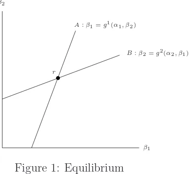
A:β₁=g1(α₁, β₂)

B:β₂=g2₍α₂, β₁)

r

Figure 1: Equilibrium

of person 2, and curve B represents the response of person 2 to β1. The

equilibrium point is r.

Claim 5 The equilibrium point of eq. (4) is unique.

Proof: Suppose that for a given vector αthere are two different equilibrium vectorsβ andβ′. Note that if for somek,β′_j6=k=β_j6=k, thenβk =βk′. There

is therefore k for which _|β′_j6=k−β_{j6=k| 6}= 0.

Next, there is j∗ such that _|βj′∗ −βj∗| > |β

′

j6=j∗ −β_j6=j∗| > 0. To see why, observe that β′_j6=j∗ −βj6=j∗ = _n−1₁

P

j6=j∗[β_j′ − βj]. If β

′

j6=j∗ > βj6=j∗, then there is j∗ _{such that β}′

j∗−βj∗ > β

′

j6=j∗ −βj6=j∗, and if β

′

j6=j∗ < βj6=j∗, then there is j∗ _{such that β}′

j∗ −βj∗ 6 β

′

j6=j∗ −β_j6=j∗. The adjustment rule for person j∗ stands in contradiction to the assumption that g2 < 1, since

β′

j∗−βj∗ =g(α_j∗,β

′

j6=j∗)−g(αj∗,β_j6=j∗).

We now analyze some specific situations in order to get a better insight into the nature of the function g.

4.1

Identical Agents

if αi = αj but βi > βj, then by the assumption that g2 > 0 it follows

that βj = g(α,_n−1₁(βi + P_k6=i,jβk)) > g(α,_n−1₁(βj +P_k6=i,jβk)) = βi, a

contradiction.

DefineG(α) to be the behavioral equilibrium when all agents’ core pref-erences are α, that is, G(α) satisfies

G(α) = g(α, G(α)) (5)

(Recall that when each of the other n ₋1 behavioral index is G(α), then so is the average of these indexes). The properties of g at the point (α, α) determine the location of G(α), above or below α. If g(α, α) = α, then so is

G(α). That is, if for each playeri, the fact that the average behavioral index of all others is identical to his core preferences does not push him to deviate from these core preferences, then in equilibrium all players will use their core preferences. Otherwise,

Claim 6 G(α)≷α iff g(α, α)≷α.

Proof: Suppose that g(α, α) > α but G(α) < α. Since g2 < 1, it follows

that

β < α=_⇒g(α, β)> β (6)

Otherwise, if g(α, β)6β, we get that g(α, α)₋g(α, β)> α₋β. Note that since G(α) is an equilibrium, it follows as in eq. (5) thatG(α) = g(α, G(α)). Since G(α)< α we get by eq. (6) that g(α, G(α))> G(α), a contradiction. Moreover, if G(α) = α, the equation G(α) = g(α, G(α)) contradicts the assumption g(α, α)> α.

Similarly, ifg(α, α)< α,G(α) cannot be aboveα, and it must be strictly

below it.

4.2

Same Influence Functions, Different Core

Prefer-ences

Claim 7 The vectors β and α are comonotonic. That is, for all i, j, (αi−

αj)(βi−βj)>0.

Proof: Suppose, for example, that αi < αj but βj < βi. Then, since

g1, g2 >0,

βi =g(αi,_n−1₁(βj+P_k6=i,jβk))< g(αj,_n−1₁(βi+P_k6=i,jβk)) =βj

A contradiction.

We want to show that it cannot be the case that the less risk averse agents will become even less risk averse while the more risk averse agents will move in the opposite direction. This follows from the stronger claim 8 below.

Definition 2 The social influence makes agents i and j more extreme if

αi < αj and βi < αi whileαj < βj.

We now show that it is never the case that two agents will move away from each other. That is, if αi < αj and αj < βj, then it is impossible that

βi < αi. Formally:

Claim 8 It is never the case that the social influence makes agents i and j

more extreme.

Proof: Consider the two profiles α = (α1, . . . , αn) and α′ = (α′1, . . . , α′n)

together with the corresponding behavioral profiles β = (β1, . . . , βn) and β′ = (β′

1, . . . , βn′), where

1. For k₆=i, j, αk =αk′ and βk =βk′,

2. α′

i =α′j =α∗ and βi′ =βj′ =β∗ := βi+βj

2 ,

3. α∗ _{is chosen such that β}∗ _=g(α∗_, 1

n−1[

P

k6=i,jβk+β∗]).

The existence ofα∗ _{is guaranteed by continuity and monotonicity. The profile}

β′ corresponds to α′ _{because for k 6=i, j, his core preferences are the same}

Suppose first that β∗ > α∗. Then αi 6 α∗. To see why, observe that if

α∗ _{< α}

i, then

βi 6β∗ = g α∗,

1

n₋1

"

X

k6=i,j

βk+β∗

#!

<

g αi,

1

n₋1

"

X

k6=i,j

βk+β∗

#!

6

g αi,

1

n₋1

"

X

k6=i

βk

#!

=βi

A contradiction. Since 0 < g1 61 andg2 >0,

g(αi,_n−1₁P_k6=iβk)>

g(αi,_n−1₁[

P

k6=i,jβk+β∗])>

g(α∗_, 1

n−1[

P

k6=i,jβk+β

∗_])

−[α∗

−αi] =

β∗₋[α∗₋αi]>αi

The proof of the case β∗ _{< α}∗ _{is similar.}

Suppose that α1 6 . . .6 αn. By claim 8, there are three possible types

of equilibria:

1. For all i, αi 6βi

2. For all i, αi >βi

3. For all i6i∗, αi 6βi, for all i > i∗,αi >βi.

We cannot give exact conditions for each of the three types to emerge, but some sufficient conditions follow. First, by claim 6, if for all α, g(α, α)> α

and all agents have the same core preferences α, then they will all have the same behavioral preferences β > α. If for a sufficient small ε, α₋ε 6α1 <

. . . < αn 6 α+ε, then by claim 7 and continuity, αn < β1 < . . . < βn (case

1 above). Case 2 is likewise obtained when for all α,g(α, α)< α.

influence yields a higher variance of the agents’ risk aversion. This is pos-sible for example when αi 6 βi for all i but the increase in risk aversion is

higher at high levels of α.

If, when the average of the observed behavior of everyone else and the decision maker’s core preference coincide the decision maker behaves accord-ing to his core preferences, then the equilibrium (for all distributions of core preferences) is of the third type. This follows by the fact that if g(α, α)_≡α, then when α1 6. . .6αn,β1 >α1 and βn6αn. To see why this is the case,

denote ˆβ = 1

n−1

P

i>1βi. By claim 7, β1 6 βi for all i > 2, hence α1 6 βˆ.

By Claim 2, the behavioral preferences of person 1 are the same if the be-havioral preferences of all other individuals are replaced by ˆβ. But g2 > 0,

α1 =g(α1, α1)6g(α1,βˆ) = β1. The proof for the caseβn 6αn is similar.

4.3

A Possible Application: Committee Deliberation

In this subsection we offer an application of our approach to the analysis of deliberation by committees or juries. Starting from Condorcet [12] there are numerous studies on decision making by committees, but the focus of this literature has been on the importance of pre-voting debates and deliberation on information aggregation. Given that committee members have different goals and preferences, this literature considers the incentives they have to reveal their private information or to acquire information (for a recent survey of this literature see Li and Suen [24]). However, efforts to convince and to persuade others are not done only by providing new information, but also by efforts to change others’ preferences regarding the subject being deliberated. To illustrate the usefulness of our setup, consider a committee that needs to vote on a certain issue, but prior to voting there is a deliberation stage. During this stage committee members explain, argue, and try to convince and influence each other. The effect of deliberation can be captured by our social influence procedure where each individual votes according to his be-havioral preferences which depend on his core preferences and the bebe-havioral preferences of committee members that participate in the deliberation.

or they may even decide not to vote at all. Voting can be done simulta-neously or sequentially (and in a different order). Adopting our setup the different procedures may affect the formation of the behavioral preferences and therefore the outcome of the committee’s voting.

5

Discussion and Concluding Comments

The approach taken in this paper is that humans are social animals that keep interacting with one another. The interaction does not affect only payoffs but also preferences. We depart from the approach that takes humans as given with fixed preferences and adopt a framework in which preference changes depend on social interaction and social influence. Our approach tries to capture the effect of social interaction on preferences and behavior without introducing any strategic or evolutionary purpose for such an influence.

There are two important assumptions in our setup: symmetry and ob-servability. One can extend our setup and consider a model in which each individual is affected only by a subset of individuals. This can be captured by mapping the details of social influence into a directed social network such there is a directed link between player i and j only if player i affects the preferences of player j. We can go further and assume that the weight of each link in the sphere of social influence is different. The social influence equilibrium for this case can be defined in the same way as in Definition 1 while restricting the formation of behavioral preferences to the specific struc-ture of the weighted directed network. The sensitivity of the distribution of behavioral preferences to the structure of the social network is potentially interesting.

Our second assumption of full observability can also be modified. One can assume that individuals have beliefs about the behavioral preferences of other individuals and they update those beliefs whenever they observe behavior. The influence function is then defined as a function of one’s core preferences and his beliefs about the preferences of others.

We focused in our analysis on risk aversion as our leading example. But as we pointed out in the introduction, the literature on social psychology suggests that group interaction affects different types of attitudes and pref-erences; a phenomenon labeled as group polarization. Our approach is there-fore also relevant in the discussion of preferences for competition and equality which have been the focus of recent economic literature (see for example Fehr and Schmidt [17] for inequality aversion and Niederle and Vesterlund [28] for a discussion on preferences for competition)). That is, when agents with given preferences for competition interact with others, they may find themselves at the end of the interaction with different attitudes towards competition from those they had at the beginning. It would be interesting to investigate under what type of social influence group interaction makes people more competitive, or make them more (or less) averse to inequality.

References

[1] Ariely, D. and J. Levav, 2000. “Sequential choice in group setting: Tak-ing the road less traveled and less enjoyed,” Journal of Consumer Re-search, 27:279–290.

[2] Aronson, E., 2010. Social Psychology. Prentice Hall: Upper Saddle River, NJ.

[3] Becker, G.S., 1970. “Altruism, egoism and genetic fitness: Economics and sociobiology,” J. Econ. Lit. 14:817–826.

[4] Bernheim, D.B., 1994. “A Theory of conformity,” Journal of Political Economy, 102:841–877.

[5] Bisin A, and T. Verdier, 2001. “The Economics of Cultural transmission and the dynamics of Preferences,” Jour. of Econ. Theory, 97:298–319.

[6] C. Blackorby, D. Primont, and R.R. Russell, “Duality, Separability, and Functional Structure: Theory and Economic Applications,” North-Holland, New York, 1978.

[8] Cavalli-Sforza, L.L. and M. Feldman, 1973. “Culture versus biological inheritance: phenotypic transmission from parents to children,” Amer. J. Human Genetics, 25:618–637.

[9] Chamley, C., 2004.Rational herds: Economic models of social learning. Cambridge University Press..

[10] Charness, G. and P. Kuhn, 2011. “Lab labor: What can labor economists learn in the lab?,” Handbook of Labor Economics, Volume 4a, 229–330.

[11] Cole, H.L., G.J. Mailath, and A. Postlewaite, 1992. “Social norms, sav-ings behavior, and growth,” Journal of Political Economy, 100:1092– 1125.

[12] Condorcet, M.J.A.N. de Caritat, 1785. “An essay on the application of analysis to the probability of decisions rendered by a plurality of voters,” abridged and translated in I. McLean and A.B. Urken, eds. Classics of

Social Choice, 1995. Ann Arbor: University of Michigan Press.

[13] Dawkins, R., 1976. The Selfish Gene, Oxford University Press, Oxford.

[14] De Finetti, B., 1977. “Probabilities of probabilities: A real problem or a misunderstanding?” in New Developments in the Applications of Bayesian Methods, ed. by A. Aykac and C. Brumat. Amsterdam: North Holland.

[15] Dunford N. and J.T. Schwartz, 1958. Linear Operators, Vol. 1. Wiley-Interscience: New York

[16] Fehr, E. and S. G¨achter, 2000. “Fairness and retaliation: The economics of reciprocity,” Journal of Economic Perspectives 14:159–181.

[17] Fehr, E. and K. M. Schmidt, 1999. “A theory of fairness, competition and Cc-operation,” Quarterly Journal of Economics 114:817–868.

[18] Fershtman, C., K.M. Murphy, and Y. Weiss, 1996. “Social status, edu-cation, and growth,” Journal of Political Economy, 104:108–132.

[20] Frank, R., 1987. “If Homo Economicus could choose its own utility func-tion: would he want one with a conscience?” Amer. Econ. Rev. 77:593– 604.

[21] Gul, F. and W. Pesendorfer. “Interdependent preference models as a theory of intentions,” Journal of Economic Theory, forthcoming.

[22] Hoff, K. and J.E. Stiglitz, 2015. “Striving for Balance in Economics: Towards a Theory of the Social Determination of Behavior,” Journal of Economic Behavior and Organization, forthcoming.

[23] Karni E. and D. Schmeidler, 1990. “Fixed Preferences and Changing Tastes,” American Economic Review: Papers and Proceedings 80:262– 267.

[24] Li, H. and W. Suen, 2009.“Decision making in Committee,” Canadian Journal of Economics 42:359–392.

[25] Mailath G.J. and A. Postlewaite, 2003. “The social context of economics decisions,” J. Eur. Econ. Assoc. 1:354–362.

[26] Myers, D.G., 1975. “Discussion-induced attitude polarization,” Human Relations 28:699–714.

[27] Myers, D.G. and H. Lamm, 1976. “The group polarization phe-nomenon,” Psychological Bulletin 83:602–627.

[28] Nierdele, M. and Vesterlund, 2007. “Do women shy away from compe-tition? Do men compete too much?” Quarterly Journal of Economics

122:1067–1101

[29] Postlewaite, A., 2001. “Social arrangements and social behavior,” Ann. Econ. Stat. 63-64:67–87.

[30] Postlewaite, A., 2011. “Social norms and social assets,” Annu. Rev. Econ. 3:239–59.

[31] Samuelson, L., 2001. “Introduction to the Evolution of Preferences,”

Journal of Economic Theory, 97:225–230.