A practical implementation of Robust Evolving Cloud based Controller with normalized data space for heat exchanger plant

A Practical Implementation of Robust Evolving

Cloud-based Controller with Normalized Data

Space for Heat-Exchanger Plant

Goran Andonovski

Plamen Angelov

School of Coputing and Communications Lancaster University, United Kingdom

[email protected]

Saˇso Blaˇziˇc, Igor ˇSkrjanc

[email protected], [email protected]

Abstract—The RECCo control algorithm, presented in this article, is based on the fuzzy rule-based (FRB) system named ANYA which has non-parametric antecedent part. It starts with zero fuzzy rules (clouds) in the rule base and evolves its structure while performing the control of the plant. For the consequent part of RECCo PID-type controller is used and the parameters are adapted in an online manner. The RECCo does not require any off-line training or any type of model of the controlled process (e.g. differential equations). Moreover, in this article we propose a normalization of the cloud (data) space and an improved adaptation law of the controller. Due to the normalization some of the evolving parameters can be fixed while the new adaptation law improves the performance of the controller in the starting phase of the process control. To assess the performance of the RECCo algorithm, firstly an comparison study with classical PID controller was performed on a model of a plate heat-exchanger (PHE). Tunning the PID parameters was done using three different techniques (Ziegler-Nichols, Cohen-Coon and pole placement). Furthermore, a practical implementation of the RECCo controller for a real PHE plant is presented. The PHE system has nonlinear static characteristic and a time delay. Additionally, the real sensor’s and actuator’s limitations represent a serious problem from the control point of view. Besides this, the RECCo control algorithm autonomously learns and evolves the structure and adapts its parameters in an online unsupervised manner.

I. INTRODUCTION

Nowadays, control of nonlinear and complex processes is still an active research topic. Besides changing circumstances, process dynamics and complexity of the processes the indus-trial markets require high and satisfactory performance of the controller. A local linear approximation of the process com-bined with the classical PID controller provides good results but only in the neighborhood of the linearized operating point while this approach is not suitable for the whole operating range of the nonlinear process.

To solve the problem of nonlinearity the authors in [1] presented a self-tuning method for a class of nonlinear PID control systems based on Lyapunov approach. Another scheme in [2] is presented where the just-in-time learning technique is employed to predict the process dynamics and furthermore, the Lyapunov method for adapting the PID parameters is used. There are many other techniques and methods, for

example, in [3] an online adaptation of PID controller using neural networks is proposed and in [4] the genetic algorithm for finding the optimal PID parameters is applied. Also the particle swarm optimization for tunning the parameters of PID controller in [5] is used. Another type of PID controllers are Fractional Order PID (FO PID) controllers that perform better than a classical PID-s [6] but require setting of two additional parameters. Similar to classical ones, tunning of this parameters can be solved by solving an optimization problem [7], [8], [9].

Fuzzy systems represent control scheme which is developed to deal with the nonlinear processes and due to their powerful adaptability and nonlinear modeling capability they are widely used in many applications [10], [11], [12], [13], [14], [15], [16], [17]. The author of fuzzy sets/systems is Prof. Lotfi A. Zadeh who firstly introduced the theory in [18]. After Prof. Zadeh has introduced the theory of fuzzy sets, Mamdani in [19] published the first fuzzy model based control applica-tion on dynamic plant (a model of steam engine). Another fuzzy control system is Takagi-Sugeno (TS) fuzzy approach proposed in [20] that has attracted lots of attention after the publication. The wide popularity and usage of the fuzzy control systems is presented in [21] where a lot of fuzzy control schemes are discussed. Similar to TS fuzzy models a new Tensor product (TP) models were developed. One of the advantages of the TP models is that the linear matrix inequality (LMI)-based control design can be applied directly to TP models. Recently, several process control solution using TP models were proposed for different applications [22], [23], [24], [25].

TABLE I

A COMPARISON OF DIFFERENT TYPES OF FRB [26]

ANTECEDENT (IF)

CONSEQUENT (THEN)

DEFUZZI-FICATION

Mamdani

[19] Fuzzy sets (scalar,

parame-terized)

Fuzzy sets (scalar,

parame-terized)

Center of Gravity

TS [20]

Functional (often linear)

Fuzzily weighted sum

ANYA [26]

Dataclouds

(non-parametric)

Any of the above

two types

the case of Mamdani systems (see Table I).

Besides the classical fuzzy rule-based (FRB) systems, TS and Mamdani, Angelov and Yager proposed a new simplified type of FRB system named ANYA in [26]. Moreover, they presented a new concept how the antecedent part is defined. As we have already mentioned above in both classical FRB systems the antecedent part is fuzzy and uses predefined and fixed membership functions of triangular, trapezoidal, Gaussian type etc. ANYA FRB system extracts the information from the real data and form the data clouds to define the membership function. The clouds are sets of data that have common properties (they are close to each other in the data space). All data have different degree of memberships to the existing clouds determined by the local density of the data sample to alldata from the particular cloud.

In [26] the authors distinguished between the clouds and the clusters and they pointed out the main differences between them. In general, the clouds do not requirea prioriinformation about the total number of membership functions or even an assumption about its form (do not have boundaries). More-over, data clouds represent allprevious data samples that are associated with the cloud.

Inspired and motivated by the simplicity of the ANYA FRB system several approaches on process control were developed and tested on different simulation models [27], [28] and on a real plant [29]. Firstly, in [27] a new fuzzy controller RECCo (Robust Evolving Cloud-based Controller) was introduced. The main advantage of the RECCo controller is that it does not require any information and knowledge about the controlled process (e.g. in a form of differential equations). Furthermore, it is initialized from the first data sample and learns autonomously while performing the control of the plant. Also the structure of the RECCo is not predefined butevolves

in an online manner during the process control (adding new clouds – fuzzy rules). In [27] and [29] a new cloud is added according to the global density of the data while in [28] and [30] a simpler way using local density threshold is proposed. Finally, controller’s parameters in the consequent part are also tuned andadapted autonomously using stable gradient-based learning method.

In this paper we propose an improvement of the RECCo controller presented in [28]. Our idea is by using the basic knowledge from the controlled process (input and output range, time constant and sampling time) to set/fix the initial parameters required by the algorithm. A new normalized data space is proposed and due to this the evolving parameter

γmax can be fixed (γmax defines ’when’ a new cloud is

added and will be introduced later in more detail). Also the adaptation gain vector ααα could be calculated using the range of the control variable and the default value. Thus the controller tuning is simplified which makes the approach more appealing for the use in practical applications. Different initial real life scenarios were analyzed and new improved adaptation law with absolute values in the starting phase is proposed to improve the performance of the controller [31]. This improvement speed up convergence and reduce large transients when the initial are far away from the unknown parameters.

In order to show the effectiveness of the proposed controller, we provide several experiments on a real plate heat-exchanger (PHE) plant and on a PHE model. Firstly, we compared the performance of the proposed algorithm RECCo with the classical PID controller on PHE model. The parameters of the PID were tunned using Ziegler-Nichols [32], Cohen-Coon [33] and by pole placement method [34]. Nowadays, the PHE is widely used in many different industries and it is suitable to apply for heating, cooling systems, heat-ventilation-air-condition (HVAC) system, in chemistry, pharmacy, food and beverages industry etc. The basic concept of the PHE is transferring the heat between two liquids (separate circuits) flowing on either side of thin metal plates. The dynamical characteristic of the PHE contains strong nonlinear behavior in gain and time constant and has time delay.

The remainder of this paper is organized as follows. In Section II the RECCo algorithm is presented, including the evolving structure and the adaptation law of the controller. The normalized data (cloud) space is explained in Section III and moreover, several experiments are provided to prove the benefit of the proposed approach. In Section IV the performance comparison between RECCo and PID controller is presented. Moreover, the PHE process is explained and the experiment is provided to show the performance and the ability of learning of the RECCo controller in practice. At the end in Section V the conclusions are given.

II. ROBUSTEVOLVINGCLOUD-BASEDCONTROLLER

(RECCO) A. The structure of the RECCo controller

gains are adapted and, if the certain conditions are satisfied, a new data cloud (fuzzy rule) is added.

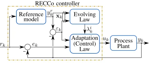
Reference

rk ek

model EvolvingLaw

Adaptation

(Control) Process_Plant yk

uk

yr k

εk λi_k

RECCo controller

xk

Law

Fig. 1. Control scheme of the RECCo algorithm.

The robust evolving cloud-based controller (RECCo) is a type of ANYA fuzzy rule-based system with non-parametric antecedents (IF part). As we mentioned above, this method applies the concept of fuzzy data clouds and normalized relative data density to define the membership of the current data1 _{to the existing clouds. The clouds represent sets of} previous data samples which are close to each other. Incoming data samples are analyzed in an online manner and each sample is associated with one of the clouds and only the parameters of that cloud are updated.

As we already said, the RECCo controller is based on the ANYA FRB system proposed in [26] and has the following form:

Ri_{: IF (x∼X}i_{) THEN (u}i₎

(1)

where the number of rules Ri _{is equal to the number of}

the clouds in the data space i = 1, . . . , c, and moreover, it changes during the control process. The non-parametric antecedent part is defined with the operator∼which could be linguistically expressed as ’is associated with’ and that means that the current datax= [x1, x2, . . . , xn]T is related to theith

cloud Xi_∈

Rn. The consequent part is defined bycdifferent (partial) control actionsuifor each rule. RECCo controller can work with different forms of defuzzification such as weighted average, center-of-gravity, ”winers takes all” and some mixed forms (e.g. parameterized defuzzification).

The degree of association between the data sample x

and corresponding cloud Xi _{is measured by the normalized}

relative density as follows:

λi_k= γ

i k c

P

j=1

γ_kj

i= 1, . . . , c (2)

whereγi

k is the local density of the ith cloud for the current

datax. The local density calculation in the following subsec-tion will be explained in detail, together with the evolving law of the RECCo controller.

B. The procedure of the RECCo control algorithm

1) Reference model: Choosing an appropriate reference model is a very important part of the proposed adaptive

1_{Data will be used to express singular and plural form in this paper}

system design. General suggestions for selecting the reference model dynamics are that the time constants have to be similar (usually slightly shorter) to those of uncontrolled process. The reference model order would be at less or equal to the order of the plant [35]. Furthermore, the initial conditions of the reference model would then need to have the same values as the initial plant (y0r=y0).

The reference model part of the RECCo controller defines the desired trajectoryyr

kand the dynamics that the plant output

ykshould follow. In this case we define simple first order linear

reference-model as:

yr_k+1 =arykr+ (1−ar)rk 0< ar<1 (3)

where the parameter ar is the pole of that model. It can be

approximated by(1−Ts

τ ), whereTsis the sampling period of

the process andτ is the time constant of the reference model which is slightly shorter than the estimated time constant of the controlled plant. In (3) the rk is the reference signal and

they_krrepresents the desired trajectory of the plant outputyk.

The goal of the controller, is to provide efficient performance and to ensure that the tracking error:

εk =yrk−yk (4)

is as small as possible (in the presence of disturbances and modeling errors).

When dealing with adaptive and evolving (online learning) systems we need to construct reference with changing steps in some operating range [rmin, ramx]. In this case the user

(operator) of the process only chooses the limit values rmin

and rmax and the RECCo algorithm constructs the step

changes in this interval.

We have to note here that the RECCo controller is not limited only to this type of reference model (first order linear model), but also other types could be used according to the dynamics of the controlled process.

2) Evolving law: The evolving law in this paper consists only a mechanism for adding new clouds (rules). Beside this, another evolving mechanisms such as merging, splitting and removing clouds can be also implemented. We decide to use just adding mechanism due to simplicity of the implementation and because it is sufficient for control the plant proposed in Section IV. The adding mechanism relies on the local density

γi

k of the current data sample with the existing clouds. The

local density takes into considerationallthe data samples from one particular cloud (therefore local) and is calculated using a suitable kernelK:

γ_ki =K 



Mi

X

j=1

di_kj



 (5)

where Mi _{is the number of data samples in i}th _{cloud and}

di

kj is the distance between the current data sample xk and

the jth _{sample x}i

j from the ith cloud. In all the equations

the superscript in variables (e.g.iinxi

k) refers to the clouds,

we can see in (5) this approach directly takes into account all previous data samples.

In this article we used a Cauchy kernel as was proposed in [26] and the local density of the i-th cloud is defined as follows:

γki =

1

1 +

PM i j=1(dikj)2

Mi

(6)

where PMi

j=1(d

i kj)

2 _{is the sum of the square of Euclidean}

distances (di_kj =kxk −xijk

2_{) between the new datax}

k and

all data points of the i-th cloud. We have to mention that, another type of distance measure could also be used (e.g. Mahalanobis in [30]) and it was shown that both Euclidean and Mahalanobis distance produced satisfying results. For easier practical and computational implementation, local density (6) can be recursively rewritten as follows:

γ_ki = 1

1 +kxk−µikk2+σ i k− kµ

i kk2

(7)

where µi_k is the mean value of the cloud’s data points and

σ_ki is the mean-square length of the data vectors in the

ith _{cloud. Both of them can be recursively calculated using}

following equations for mean value and mean-square length, respectively:

µik=

Mi−1

Mi µ

i k−1+

1

Mixk (8)

σ_ki =M

i₋₁

Mi σ

i k−1+

1

Mikxkk

2 ₍₉₎

Initial condition (Mi_{= 1) for the mean value isµ}i

1=x1and for the mean-square length is σi

1=kx1k2.

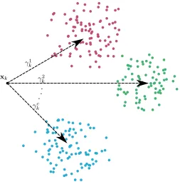
The evolving law in this paper consists the mechanism of adding new clouds and is the same as the one presented in [28]. Moreover, it is much simpler in comparison to the mechanism used in [27], [29]. Once a new data sample arrive we need to calculate c different local densities between the sample and all the existing clouds (see Fig. 2). According to the maximal local density (maxiγki) the data sample is associated

with that cloud and furthermore, the parameters of that cloud are updated using equations (8) and (9). Theoretically, it is possible to happen that the current data sample has the same density to two or more clouds. In that case we associate that data sample with the oldest cloud (the one that was added before the others). But, if the maximal local density (maxiγki)

is lower than the threshold valueγmax(the current data sample

is far away from all existing clouds), a new cloud is added. The cloud’s data space is normalized (it will be explained in the next section) and due to this the default value of the threshold can be fixed γmax = 0.93. Some conservatism is

always welcome when changing the structure of the evolving system. This is why some other criteria need to be fulfilled before adding a new cloud (such as certain time nadd has

passed from the last change). We have to note here that in our previous and current experiments we always use default value of this parameter nadd= 20. Moreover, because of the

normalized data space and fixed value of the parameter γmax

the adding of new clouds is more stable and the parameter

nadd can be even neglected. We can summarize the whole

evolving procedure presented above in the pseudo Algorithm 1 (see lines from 9 to 22).

xk

γ1

k

γ_k2

γc k

Fig. 2. Associating the current data samplexkwith one of the existing clouds according to the local densitiesγi_k, wherei= 1, . . . , c

3) Adaptation law: For the consequent part of the RECCo controller the PID-type control is used [28] and each cloud (fuzzy rule) has its own PID parameters. The vector of the pa-rameters is denoted asθ_ki =P_ki, I_ki, D_ki, Ri_kT and parameters of the first cloud are initialized with zerosθ01 = [0,0,0,0]

T

, while all later added clouds are initialized with mean value of the parameters of all previous clouds as follows:

θ₀c= 1

c−1

c−1 X

j=1

θ_kj (10)

wherecis the index of the newly added cloud.

After the classification of the current data sample to one of the clouds, only the PID parameters of that cloud are adapted while the parameters of other clouds are kept constant:

θik=θik−1+ ∆θki (11)

Algorithm 1 Pseudo code of the RECCo PID control algo-rithm

1: Initialize (Process parameters):τ,Ts,umin,umax,rmin,

rmax.

2: Initialize (Evolving parameters):γmax,c= 0,cmax,nadd. 3: Initialize (Adaptation parameters):αP,αI,αD,αR, σL,

ddead,θ,θ. 4: repeat

5: Measurement: yk. 6: Define and compute:yr

k . Reference model 7: Compute:ek,εk,Σεk,∆εk.

8: Compute:xk= [ εk/∆ε, (yrk−rmin)/∆r] T

.

9: if c= 0 then . Start of the evolving law

10: Increment:c,

11: Store:kadd,

12: Initialize:µ10,σ01,θ10.

13: else

14: Calculate:γi k,λ

i

k, wherei= 1, . . . , c

15: if(maxiγki < γmax andk >(kadd+nadd))then

16: Increment:c,

17: Store:kadd,

18: Initialize: µc

0,σc0,θc0.

19: else

20: Associate samplexk with cloud (maxiγik)

21: Updateµi

k,σki for the cloud (maxiγki) 22: end if

23: end if . End of the evolving law

24: Adaptation of thePID controller gains.

25: Computation of the control law.

26: untilEnd of data stream.

follows:

∆P_ki=αPGsignλik

|ekεk|

1 +r_k2

∆I_ki =αIGsignλik

|ek∆εk|

1 +r2

k

∆D_ki =αDGsignλik

|ek∆εk|

1 +r2

k

∆Ri_k =αRGsignλik

εk

1 +r2

k

(12)

where αP, αI, αD, αR are the adaptation gains of the

con-troller parameters, Gsign = ±1 is the known process gain

sign, λi_k is the normalized local density of the cloud, εk

is the tracking error while the control error is denoted as

ek =rk−yk. The discrete-time derivative is denoted as ∆εk

and will be discussed later. In (12) only the adaptation gains should be set initially. The default value of the parameters is 0.1 and is used when the range of the control variable is (umin = 0/4, umax = 20). When the range is different, the

value of the parameters is scaled as follows:

αnew=

umax−umin

20 ·0.1

For example if the range is from umin = 0 to umax = 100

the new value of the adaptive gains will be αnew= 0.5.

0 10 20 30 40 50 60

20 25 30 35 40 45 50 55

t[min]

[

◦C

]

rk

yr k

yk

0 10 20 30 40 50 60

20 25 30 35 40 45 50 55

t[min]

[

◦C

]

rk

yr k

yk

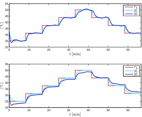
Fig. 3. The reference, the model reference and the controlled signal for heat-exchanger pilot plant in the starting phase with (upper plot) and without (lower plot) calculating the absolute value in adaptation law of the controller gains (y0= 32◦C, r0= 25◦C).

The absolute values in (12) are used only in the starting phase of the control performance (five time constants is enough) and after that they are omitted from the adapta-tion law. The problem appears when the initial value of the controlled variable is higher than the reference value (y0 > r0) which causes negative control error (ek < 0)

and correspondingly negative adaptation of the parameters (∆Pi

k,∆Iki,∆Dik < 0). As we already mentioned, the

pa-rameters of the first data cloud are initialized with zeros and without the absolute values in (12) the negative adaptation will lead to even bigger error. Fig. 3 shows the difference in the control performance with and without using absolute values in the starting phase. On the other hand, this adaptation law does not alter the performance of the controller in the case of the positive initial error, moreover, does not depend on the signGsign of the process gain.

In the section I we noted that the proposed approach can work with both TS and Mamdani (Table I) rule consequent part. For a PID-type controller, the rule consequent has the following form:

ui_k=P_kiεk+IkiΣ ε k+D

i k∆

ε k+R

i

k, i= 1, . . . , c (13)

where P_ki, I_ki, Di_k are controller gains while R_ki is compen-sation of the operating point. While the adaptation of the parameter Ri_k in (12) is driven only by tracking error εk

this parameter tries to correct the offset error of the current operating point.Σε

k and∆ ε

k in (13) are discrete-time integral

and derivative of the tracking error, respectively, and can be calculated as follows:

Σ_kε=

k−1 X

κ=0

εκ=Σkε−1+εk−1 (14)

Finally, for the defuzzification the weighted average is used (but not limited to this form) and furthermore, the control variable becomes:

uk=umin+ c

X

i=1

λi_kui=umin+ c

P

i=1

γi kui

c

P

i=1

γi k

(16)

where ui denotes the i-th (partial) rule consequent and normalized relative density (2) is used. From the practical implementation point of view we adduminin this equation (in

comparison with the one proposed in [27], [28]) and represents the minimal input value of the real actuator which in our case is umin= 4 mA.

C. The instability protection mechanism

This subsection is devoted to the modifications of the adap-tation law (11) that improve the robustness of the closed-loop system. Supervised adaptation of any controller can improve, theoretically and practically, the performance and robustness of the controller. In order to minimize the negative influence of parasitics, disturbances in the system and to eliminate the pure integral action of the adaptive law, we introduce several mechanisms to improve the RECCo control algorithm.

When dealing with adaptive controllers and parameter adaptation we need to be aware of the potential instability problems caused by the parameter drift [36]. Due to this, to make RECCo controller more robust, several techniques were already applied in [27] and [28]. In this paper we will use the following techniques:

1) Dead zone in the adaptation law: To improve the robust-ness under the unknown bounded disturbances and modeling errors, the RECCo controller includes a dead-zone in adapta-tion law. The general idea behind the dead-zone mechanism, in case of bounded disturbances, is to turn off the adaptation algorithm when the absolute value of the tracking error is smaller than a certain threshold [37]:

∆¯θki =

( ∆θi

k |εk| ≥ddead

0 |εk|< ddead

i= 1, . . . , c (17)

The parameter ddead should be chosen slightly larger than

the process noise to improve the effectiveness of the adaptive law. A larger threshold implies a shorter adaptation period and larger tracking error, while smaller value can lead to parameter drift.

2) Parameter projection: Parameter projection mechanism is used to guarantee that the estimation of the parameters will stay within finite known region [38]. In the case of the positive plant gain all the parameters should be bounded by 0 from bellow while upper bound may or may not be provided. The adaptive law in (11) is generalized as follows:

θi_k=   

 

θi

k−1+ ∆θ

i

k θ≤θ

i

k−1+ ∆θ

i k≤θ

θ θi

k−1+ ∆θki < θ

θ θi

k−1+ ∆θ

i k > θ

i= 1, . . . , c

(18)

In our case we choseθ= 0andθ=∞for the controller gains

Pk,Ik, andDk, while for the compensation of the operating

pointRk the lower bound was θ=−∞. If we have some a

priori knowledge where the true parametersθ∗ are located in Rn_{we can define upper and lower bound for the elements ofθ.}

The benefit of such information may speed up the convergence of finding optimal parameters.

3) Leakage in the adaptation law: The use of leakage in the adaptation law is a very known approach for improvement of robustness of adaptive control. Already exist different types of leakage, for example σ-modification [39],e1-modification [40], switchingσ-modification [41] etc.

Including the leakage in the adaptation law results in:

θi_k= (1−σL)θik−1+ ∆θ

i

k i= 1, . . . , c (19)

whereσL defines the extent of the leakage.

4) Interruption of adaptation: In the RECCo algorithm we first calculate the adaptation of the PID parameters (∆θi

k) and

then the control variable uk. In some cases this two steps

can be in conflict, which means that the adaptation causes control signal which is outside the limits[umin, umax]. In such

case the adaptive law should be interrupted in the following manner:

∆¯θik=

( ∆θi

k umin≤uk≤umax

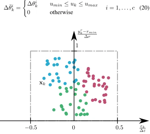
0 otherwise i= 1, . . . , c (20)

y_kr−rmin

∆r

1

0 εk

∆ε

−0.5 0.5

xk

Fig. 4. Normalized cloud space.

III. CLOUD SPACE NORMALIZATION

Until now, we did not discuss the content and the definition of the data sample xk. In the previous work [28] the data

sample was defined in 2D space as xk = [εk, ykr] T

, where the first element (εk) represents the horizontal axis while the

second element (y_kr) represents the vertical axis of the data space. In this case, if we want to change the operating range of the reference signal rk, this will also affect the reference

model outputyr

k, and consequently the data space will change

its size (shrink or expand) in both direction (yr

Our idea is to define a constant data space (see Fig. 4), where majority of the data will appear, regardless of the range of the reference signal. Even if we want to control a different process, the same data normalization can be used with the same constant data space. As a consequence, the evolving parameter γmax can be fixed. We propose a normalized data

space as follows:

x=h εk

∆ε, yr

k−rmin

∆r

iT

(21)

where ∆r = rmax−rmin and ∆ε = ∆₂r. In this case the

operator (user) needs to choose, according to the process re-quirements, only the operating range of the plant[rmin, rmax].

After that, several step changes of the reference signal rk are

constructed to cover the whole range of the process (e.g. see upper plot in Fig. 12).

IV. EXPERIMENTAL RESULTS OF A HEAT-EXCHANGER PILOT PLANT

A. Comparison between RECCo and classical PID controllers

In this subsection, the performance of the RECCo con-troller in comparison with the classical PID concon-troller is studied. Three methods for designing the parameters of the PID controller were used: Ziegler-Nichols [32] (P IDZN),

Cohen-Coon [33] (P IDCC) and pole placement method [34]

(P IDP P). To verify the performance of the proposed control

algorithm a model of plate heat-exchanger (PHE) was used [42]. The control procedure of the RECCo controller for PHE model is described in [43]. The same procedure for acquiring the parameters and the structure of the RECCo controller in this paper was used.

From the open loop response of the PHE model (see Fig. 5), the characteristic parameters such as process gain KP,

time constants τP and dead time Tdead,P were obtained. Due

to the non-linearity of the process model, each operating point has different characteristic parameters (see Table II). An exception is the dead time which is constant. For the gain and the time constant of the process we calculate average value. Therefore, the average process gain is KP = 2.49 while the

average time constant is τP = 35.25. This parameters were

used to determine the values of the PID controllers (P IDZN,

P IDCC, andP IDP P). The sampling time used isTs= 2 s.

0 50 100 150

t[min]

0 10 20 30 40 50 60

yk[◦C]

uk[mA]

Fig. 5. Simulation. Open-loop response of the plate heat-exchanger model.

TABLE II

SIMULATION. PROCESS CHARACTERISTICS OF THEPHEMODEL: PROCESS GAINKP,TIME CONSTANTτ,AND DEAD TIMEtdead.

uk[mA] 6 8 10 12 14 16 18 20

KP 3.38 4.17 4.93 2.71 1.21 1.73 1.10 0.68

τP[s] 48 50 27 19 18 47 44 29

Tdead,P[s] 4 4 4 4 4 4 4 4

For the performance evaluation, several criteria functions were compared, such as maximum overshoot, rising and settling time. Furthermore, the control effort was evaluated using integral criteria functions: Sum of the Absolute Input differences (fSAdU) and Sum of the Squared Input differences

(fSSdU):

fSAdU =

X

k

|∆uk| (22)

fSSdU =

X

k

∆u2_k (23)

where∆uk=uk−uk−1 is a change of the input action. Besides evaluating the control effort, we also compared integral (cumulative) of the process error (ek=rk−yk) using

the following criteria functions:

fSAE=Ts

X

k

|ek| (24)

fSSE=Ts

X

k

|e2_k| (25)

whereTs is the sampling time and in our case is equal to 2.

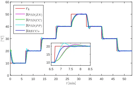
Finally, the comparison results are presented in the next figures and tables. First, in Fig. 6 the controlled variables ob-tained by each of the controllers (P IDZN,P IDCC,P IDP P

andRECCo) are presented.

0 5 10 15 20 25 30 35 40 45 50

t[min] 0

10 20 30 40 50 60

[

◦C

]

rk

yP ID(ZN)

yP ID(CC)

yP ID(P P)

yRECCo

6.5 7 7.5 8 8.5

10 15 20

Fig. 6. Simulation. The comparison of the responses (controlled variables) obtained by different controllers.

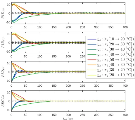
For better comparison, the same controlled variables form Fig. 6 are also shown in Fig. 7 where the different operating points are plotted in the same time frame. The rise time (the time required by the response yk to rise from 10 % to 90 %

is smaller than 0.25◦C) were calculated and the results are presented in Table III. Focusing on the rise time from the table, in some cases the pole placement controller provide better results, but the difference is in range of few time samples. Comparing the maximal overshoot and the settling time the RECCo controller provides better results.

0 50 100 150 200 250 300 350 400

-10 0 10

P

I

D

Z

N

0 50 100 150 200 250 300 350 400

-10 0 10

P

I

D

C

C

0 50 100 150 200 250 300 350 400

-10 0 10

P

I

DP

P

0 50 100 150 200 250 300 350 400

trel[sec]

-10 0 10

R

E

C

C

o

yk:rk(10→20 [◦C]) yk:rk(20→30 [◦_C])

yk:rk(30→40 [◦_C])

yk:rk(40→50 [◦_C])

yk:rk(50→40 [◦C]) yk:rk(40→30 [◦C]) yk:rk(30→20 [◦C]) yk:rk(20→10 [◦C])

Fig. 7. Simulation. Each of the four plots shows the performance of a controller in 8 different transients of the controlled variable (all the transients are appropriately shifted).

TABLE III

SIMULATION. PERFORMANCE COMPARISON BETWEEN THE FOUR CONTROLLERS FOR PLATE HEAT-EXCHANGER.

rk[◦C] 10 20 30 40 50 40 30 20

Rise time[s]

P IDZN 44 36 34 36 122 42 26 42

P IDCC 46 40 38 42 112 42 28 44

P IDP P 46 14 12 12 110 38 14 16

RECCo 42 20 24 28 104 36 22 28

Overshoot[%]

P IDZN 5.8 11.7 4.5 5.0 4.2 20.1 5.9 5.1

P IDCC 3.5 6.6 1.6 2.9 2.2 14.8 2.5 3.0

P IDP P 5.1 19.6 12.7 8.6 2.3 16.0 8.6 7.1

RECCo 1.9 1.4 1.6 1.3 2.0 6.8 1.3 2.0

Settling time[s]

P IDZN 116 98 78 94 382 168 78 100

P IDCC 122 96 54 242 154 114 68 82

P IDP P 150 238 34 48 144 102 38 74

RECCo 60 30 42 42 138 80 42 48

Table IV summarizes the comparison between the four controllers based on four criteria (22), (23), (24) and (25). We can notice that for all criteria functions the RECCo controller indicates better performance in controlling the PHE process.

B. Real system

In our experimental study a real plant of plate heat-exchanger (PHE) is used. The main purpose of this device is

TABLE IV

SIMULATION. COMPARISON BETWEEN THE FOUR CONTROLLERS USING DIFFERENT CRITERIA FUNCTIONS.

fSAdU[A] fSSdU

A2

fSAE[◦C] fSSE

◦_C2

P IDZN 2.93 18.52 1419 25430

P IDCC 2.87 18.64 1121 20277

P IDP P 1.77 9.28 327 6110

RECCo 1.59 6.48 309 5129

to efficiently transfer the heat from one medium to another. In Fig. 8 the process scheme is shown. It consists of two separate water circuits (the primary one is hot flow and the secondary is cold water flow). The primary circuit has a constant inlet temperature Tec(k) controlled by on-off thermostat which

characteristic will be discussed later. Motor driven valve V1 controls the primary circuit flow Fc(k) and represents the

control variableuk. The outlet water of the plate exchanger of

the primary circuit is returned to the reservoir. The secondary circuit has inlet temperature Tep(k) and the constant water

flow of cold water Fp(k) on one side and the controlled

variable is outlet temperature Tsp(k)on the other side of the

circuit.

Fig. 8. Plate heat-exchanger pilot plant process.

The practical implementation of the whole system (RECCo control algorithm, Data Acquisition System and PHE Plant) for process control is shown in Fig. 9. We can notice that RECCo algorithm requires only two connections to the real process,

uk andyk, without additional information of the process. The

control signal uk is in the range 4 mA – 20 mA and is not

additionally converted because both, the RECCo algorithm and the PHE process work in the same range. On the other hand, the temperature sensor provides the signal in the range4 mA –20 mAand additionally, we need to convert this signal to the actual temperature range of the sensor (from 0◦Cto100◦C) for easier interpretation and understanding of the results.

The wide hysteresis of the thermostat (approximately ±2◦_{C) in the primary circuit represents the disturbance and}

PC Matlab (RECCo)

Data Acquisition

System

PHE Pilot plant

Process 𝑢𝑢(𝑘𝑘)

𝑦𝑦(𝑘𝑘)

(4−20 mA)

Fig. 9. Process control and data acquisition system.

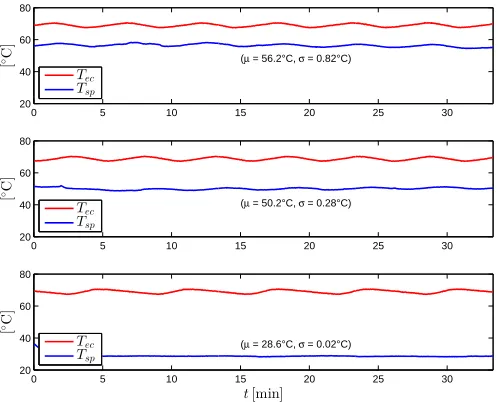
in three operating points. The variances and the mean values of the signalsTsp(k)for each operating point are then calculated.

The changing influence of the thermostat characteristics in different operating points provides an additional complexity to the process and makes the control problem more challenging.

0 5 10 15 20 25 30

20 40 60 80

(µ = 56.2°C, σ = 0.82°C)

[

◦C

]

Tec

Tsp

0 5 10 15 20 25 30

20 40 60 80

(µ = 50.2°C, σ = 0.28°C)

[

◦C

]

Tec

Tsp

0 5 10 15 20 25 30

20 40 60 80

(µ = 28.6°C, σ = 0.02°C)

t[min]

[

◦C

]

Tec

Tsp

Fig. 10. The variation of the inlet temperatureTecdue to the primary circuit thermostat at constant valve opening in three different operating points (top

uk= 20 mA, middleuk= 13.3 mAand bottomuk= 4.6 mA).

The open loop response of the plant is shown in Fig. 11. The step changes of the input signal are chosen to cover the whole range of the process (from 4 mA to 20 mA in steps of 1 mA). It can easily be noticed the nonlinearity of the process: changing time constant depending on the operating point, and also the effect of the thermostat hysteresis to the process. As already said, the effect of the thermostat is larger in the higher operating points. All these characteristics of the PHE process are dealt with RECCo controller and the results of the proposed algorithm are shown in the following.

Advantage of the RECCo controller is that we need only very basic information of the controlled process (estimated value of the dominant time constant τ, the range of the actuator [umin, umax], and the range of the controlled

vari-able [rmin, rmax]). Furthermore, the controller’s structure is

evolved and parameters are adapted during performing the control of the process. The design parameters are divided into three groups (process, evolving and adaptive parameters), the same as in the initialization phase of Algorithm 1.

0 50 100 150 200 250 300

20 40 60 80

t[min]

[

◦C

]

Tsp

Tec

0 50 100 150 200 250 300

5 10 15 20

t[min]

[m

A]

uk

Fig. 11. Open-loop response of the PHE outputTspto the series of step changes on the input valveV1 (ukchanges from4 mAto20 mAin steps of1 mA, bottom plot). Top plot shows the inlet water temperatureTec(red line) and the outlet water temperatureTsp(blue line).

1) The first group contains very technical (process) param-eters which are set according to the system requirements. The process range in this experiment was chosen as

rmin = 25◦C and rmax = 50◦C. We mentioned

above that in the case of a different process range, no additional tuning of adaptive and evolving parameters is required. The time constant and the sampling time of the reference model were chosen as τ = 40 s and

Ts= 2 s, respectively. The time constantτ is chosen in

the range of the time constant of the plant. The process input or the actuator’s range was defined by the hardware (umin= 4 mA,umax= 20 mA).

2) The evolving parameters from the second group define the rules when and why a new cloud is added. Simula-tions were started with zero fuzzy clouds (rules). A new cloud is added when the maximal value of the local densities γ_ki, i = 1, . . . , c is lower than the threshold value γmax = 0.93. The parameter that defines the

minimum number of samples between two new clouds is defined asnadd= 20.

3) The third group contains parameters of the adapta-tion/control law. The dead zone ddead was chosen as

1% of the process range∆r (ddead= 0.25◦C) and the

leakage parameter is set to σL = 10−6. All adaptive

gains αP, αI, αD andαR are set to 0.1.

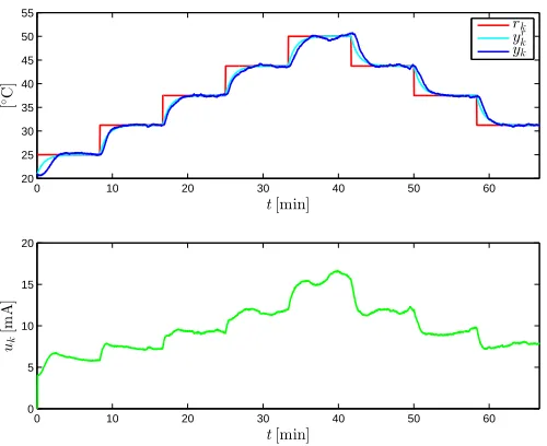
In this section the practical results are presented and the improvements of the RECCo controller (adaptation of the parameters and cloud space normalization) are tested. A closer look to the starting phase of the experiment is shown in Fig. 12 where the referencerk, the model reference outputykr, the

controlled signal yr, and the control signal uk are given. At

the phase after the transient of the adaption is shown. In Fig. 14 all added clouds during the process control are shown. In this case six clouds (fuzzy rules) have been constructed. The tracking errorεk is shown in Fig. 15 where its decreasing with

time can be clearly noticed.

0 10 20 30 40 50 60

20 25 30 35 40 45 50 55

t[min]

[

◦C

]

rk yr k yk

0 10 20 30 40 50 60

0 5 10 15 20

t[min]

uk

[m

A

]

Fig. 12. The reference, the model reference and the controlled signal (top plot) and the control signal (bottom plot) for plate heat exchanger in the starting phase.

1270 1280 1290 1300 1310 1320 1330

20 25 30 35 40 45 50 55

t[min]

[

◦C

]

rk yr k yk

1270 1280 1290 1300 1310 1320 1330

0 5 10 15 20

t[min]

uk

[m

A

]

Fig. 13. The reference, the model reference and the controlled signal (top plot) and the control signal (bottom plot) for plate heat exchanger in the finishing phase.

V. CONCLUSION

In this paper a practical implementation of the RECCo control approach on a real heat-exchanger was proposed. Moreover, a new approach of RECCo with normalized data space and improved adaptation of controller parameters was used. The normalization of the data space results in making the

−0.4 −0.3 −0.2 −0.1 0 0.1 0.2 0.3

−0.2 0 0.2 0.4 0.6 0.8 1 1.2

εk,norm

y

r k,n

o

r

m

Fig. 14. The clouds in the input spacex=

h

εk ∆ε,

yr_k−rmin ∆r

iT .

0 200 400 600 800 1000 1200

t_[min] -4

-3 -2 -1 0 1 2 3

εk

[

◦C

]

Fig. 15. The tracking errorεkfor heat-exchanger pilot plant (y0= 15◦C).

process (only the range of the control and controlled variable are needed and a rough estimate of the dominant time constant of the controlled process). This approach effectively deals with nonlinear processes.

REFERENCES

[1] W.-D. Chang, R.-C. Hwang, and J.-G. Hsieh, “A self-tuning pid control for a class of nonlinear systems based on the lyapunov approach,”

Journal of Process Control, vol. 12, pp. 233–242, 2002.

[2] Y. Kansha, L. Jia, and M.-S. Chiu, “Self-tuning PID controllers based on the Lyapunov approach,”Chemical Engineering Science, vol. 63, no. 10, pp. 2732 – 2740, 2008.

[3] C. Riverol and V. Napolitano, “Use of Neural Networks as a Tuning Method for an Adaptive PID: Application in a Heat Exchanger,” Chem-ical Engineering Research and Design, vol. 78, no. 8, pp. 1115 – 1119, 2000.

[4] A. Altinten, S. Erdogan, F. Alioglu, H. Hapoglu, and M. Alpbaz, “Appli-cation of adaptive PID control with genetic algorithm to a polymerization reactor,”Chemical Engineering Communications, vol. 191, no. 9, pp. 1158–1172, 2004.

[5] A. Moharam, M. A. El-Hosseini, and H. A. Ali, “Design of optimal PID controller using hybrid differential evolution and particle swarm optimization with an aging leader and challengers,”Applied Soft Com-puting, vol. 38, pp. 727 – 737, 2016.

[6] I. Podlubny, “Fractional-order systems and PIλ_Dµ_{−controllers,”IEEE}

Transactions on Automatic Control, vol. 44, no. 1, pp. 208–214, Jan 1999.

[7] J. A. Tenreiro Machado, “Optimal tuning of fractional controllers using genetic algorithms,”Nonlinear Dynamics, vol. 62, no. 1, pp. 447–452, 2010.

[8] J. T. Machado, A. M. Galhano, A. M. Oliveira, and J. K. Tar, “Optimal approximation of fractional derivatives through discrete-time fractions using genetic algorithms,”Communications in Nonlinear Science and Numerical Simulation, vol. 15, no. 3, pp. 482 – 490, 2010.

[9] Y. Mousavi and A. Alfi, “A memetic algorithm applied to trajectory control by tuning of fractional order proportional-integral-derivative controllers,”Applied Soft Computing, vol. 36, pp. 599 – 617, 2015. [10] Y. Bai, H. Zhuang, and Z. S. Roth, “Fuzzy logic control to suppress

noises and coupling effects in a laser tracking system,”IEEE Transac-tions on Control Systems Technology, vol. 13, no. 1, pp. 113–121, Jan 2005.

[11] I. Baturone, F. Moreno-Velo, S. Sanchez-Solano, and A. Ollero, “Auto-matic design of fuzzy controllers for car-like autonomous robots,”IEEE Transactions on Fuzzy Systems, vol. 12, no. 4, pp. 447–465, Aug 2004. [12] P. Bonissone, V. Badami, K. Chiang, P. Khedkar, K. Marcelle, and M. Schutten, “Induial applications of fuzzy logic at general electric,”

Proceedings of the IEEE, vol. 83, no. 3, pp. 450–465, Mar 1995. [13] Z. Bingul, G. Cook, A. Strauss, and K. Rashid, “Application of fuzzy

logic to spatial thermal control in fusion welding,” inIndustry Applica-tions Conference, 1999. Thirty-Fourth IAS Annual Meeting. Conference Record of the 1999 IEEE, vol. 1, 1999, pp. 627–634 vol.1.

[14] R. Boukezzoula, S. Galichet, and L. Foulloy, “Observer-based fuzzy adaptive control for a class of nonlinear systems: real-time imple-mentation for a robot wrist,”IEEE Transactions on Control Systems Technology, vol. 12, no. 3, pp. 340–351, May 2004.

[15] W.-J. Chang and P.-H. Chen,Stabilization for truck-trailer mobile robot system via discrete LPV T-S fuzzy models. Berlin, Heidelberg: Springer-Verlag, 2013, vol. 193, ch. Intelligent Autonomous Systems 12, pp. 209– 217.

[16] L. E. Ramos-Velasco, O. A. Domnguez-Ramrez, and V. Parra-Vega, “Wavenet fuzzy PID controller for nonlinear MIMO systems: Exper-imental validation on a high-end haptic robotic interface,”Applied Soft Computing, vol. 40, pp. 199 – 205, 2016.

[17] S. Fidanova and P. Pop, “An improved hybrid ant-local search algorithm for the partition graph coloring problem,”Journal of Computational and Applied Mathematics, vol. 293, pp. 55 – 61, 2016.

[18] L. A. Zadeh, “Outline of a new approach to the analysis of complex systems and decision processes,”IEEE Transactions on Systems, Man and Cybernetics, vol. SMC-3, no. 1, pp. 28–44, Jan 1973.

[19] E. Mamdani, “Application of fuzzy algorithms for control of simple dynamic plant,”Proceedings of the Institution of Electrical Engineers, vol. 121, no. 12, pp. 1585–1588, December 1974.

[20] T. Takagi and M. Sugeno, “Fuzzy identification of systems and its applications to modeling and control,”IEEE Transactions on Systems, Man and Cybernetics, vol. SMC-15, no. 1, pp. 116–132, Jan 1985. [21] G. Feng, “A survey on analysis and design of model-based fuzzy control

systems,”IEEE Transactions on Fuzzy Systems, vol. 14, no. 5, pp. 676– 697, Oct 2006.

[22] R. E. Precup, L. T. Dioanca, E. M. Petriu, M. B. Rdac, S. Preitl, and C. A. Drago, “Tensor product-based real-time control of the liquid levels in a three tank system,” in2010 IEEE/ASME International Conference on Advanced Intelligent Mechatronics, July 2010, pp. 768–773. [23] P. Baranyi, P. Korondi, and K. Tanaka, “Parallel Distributed

Compensa-tion Based StabilizaCompensa-tion of A 3DOF RC Helicopter: A Tensor Product Transformation Based Approach,”Journal of Advanced Computational Intelligence and Intelligent Informatics, vol. 13, pp. 25–34, 2009. [24] P. Grf, P. Baranyi, and P. Korondi, “Determination of the stability

pa-rameter space of a two dimensional aeroelastic system, a tp model-based approach,” in 2010 IEEE 14th International Conference on Intelligent Engineering Systems, May 2010, pp. 265–270.

[25] R. E. Precup, C. A. Dragos, S. Preitl, M. B. Radac, and E. M. Petriu, “Novel tensor product models for automatic transmission system control,”IEEE Systems Journal, vol. 6, no. 3, pp. 488–498, Sept 2012. [26] P. Angelov and R. Yager, “Simplified fuzzy rule-based systems using non-parametric antecedents and relative data density,” in 2011 IEEE Workshop on Evolving and Adaptive Intelligent Systems (EAIS), April 2011, pp. 62–69.

[27] P. Angelov, I. ˇSkrjanc, and S. Blaˇziˇc, “Robust evolving cloud-based controller for a hydraulic plant,” in2013 IEEE Conference on Evolving and Adaptive Intelligent Systems (EAIS), April 2013, pp. 1–8. [28] I. ˇSkrjanc, S. Blaˇziˇc, and P. Angelov, “Robust evolving cloud-based PID

control adjusted by gradient learning method,” in2014 IEEE Conference on Evolving and Adaptive Intelligent Systems (EAIS), June 2014, pp. 1– 8.

[29] B. Costa, I. ˇSkrjanc, S. Blaˇziˇc, and P. Angelov, “A practical implementa-tion of self-evolving cloud-based control of a pilot plant,” in2013 IEEE International Conference on Cybernetics (CYBCONF), June 2013, pp. 7–12.

[30] S. Blaˇziˇc, D. Dovˇzan, and I. ˇSkrjanc, “Cloud-based identification of an evolving system with supervisory mechanisms,” in 2014 IEEE International Symposium on Intelligent Control (ISIC), Oct 2014, pp. 1906–1911.

[31] G. Andonovski, S. Blaˇziˇc, P. Angelov, and I. ˇSkrjanc, “Analysis of adaptation law of the robust evolving cloud-based controller,” in2015 IEEE International Conference on Evolving and Adaptive Intelligent Systems (EAIS), Dec 2015, pp. 1–7.

[32] N. N. J. Ziegler, “Optimum settings for automatic controllers,” Trans-actions of ASME64, 1942.

[33] G. Cohen and G. Coon, “Theoretical consideration of retarded control,”

Transactions of ASME, vol. 75, pp. 827–834, 1953.

[34] K. J. AAstr¨om and T. H¨agglund,PID Controllers: Theory, Design, and Tuning, 2nd ed. Instrument Society of America, Research Triangle Park, NC, 1995.

[35] H. Kaufman, I. Barkana, and K. Sobel,Direct Adaptive Control Algo-rithms. New York: Springer-Verlag, 1998.

[36] C. Rohrs, L. Valavani, M. Athans, and G. Stein, “Robustness of continuous-time adaptive control algorithms in the presence of unmod-eled dynamics,”IEEE Transactions on Automatic Control, vol. 30, no. 9, pp. 881–889, Sep 1985.

[37] B. Peterson and K. Narendra, “Bounded error adaptive control,”IEEE Transactions on Automatic Control, vol. 27, no. 6, pp. 1161–1168, Dec 1982.

[38] G. Kreisselmeier and K. Narendra, “Stable model reference adaptive control in the presence of bounded disturbances,”IEEE Transactions on Automatic Control, vol. 27, no. 6, pp. 1169–1175, Dec 1982. [39] P. Ioannou and P. Kokotovic, “Instability analysis and improvement of

robustness of adaptive control,” Automatica, vol. 20, no. 5, pp. 583 – 594, 1984.

[40] K. Narendra and A. Annaswamy, “A new adaptive law for robust adap-tation without persistent exciadap-tation,” in American Control Conference, June 1986, pp. 1067–1072.

[42] I. ˇSkrjanc and D. Matko, “Predictive functional control based on fuzzy model for heat-exchanger pilot plant,” IEEE Transactions on Fuzzy Systems, vol. 8, no. 6, pp. 705–712, Dec 2000.