warwick.ac.uk/lib-publications
A Thesis Submitted for the Degree of PhD at the University of Warwick
Permanent WRAP URL:
http://wrap.warwick.ac.uk/132616
Copyright and reuse:
This thesis is made available online and is protected by original copyright.
Please scroll down to view the document itself.
Please refer to the repository record for this item for information to help you to cite it.
Our policy information is available from the repository home page.
Efficient Information Collection in
Stochastic Optimisation
by
Xin Fei
Thesis
Submitted to the University of Warwick
in partial fulfilment of the requirements
for admission to the degree of
Doctor of Philosophy
Warwick Business School
Contents
List of Tables iv
List of Figures v
Acknowledgments vii
Declarations viii
Abstract ix
Chapter 1 Introduction and Background 1
1.1 Review of Efficient Information Collection . . . 2
1.2 Structure of Thesis and Contributions . . . 5
Chapter 2 Efficient Solution Selection for Two-stage Stochastic Pro-grams 7 2.1 Introduction . . . 7
2.2 Sample Average Approximation for Two-stage Linear SPR . . . 10
2.2.1 Two-stage Linear SPR Formulation . . . 10
2.2.2 The Near-optimal Solution and its Performance Estimator . . 11
2.2.3 Solution Selection Under a Fixed Computing Budget . . . 13
2.3 Optimal Computing Budget Allocation . . . 13
2.4 Wasserstein-based Solution Screening . . . 16
2.5 Wasserstein Distance Estimation . . . 22
2.6 The Proposed Two-stage Selection Approach . . . 24
2.7 Numerical Experiments . . . 25
2.7.1 Overview of Test Instances . . . 25
2.8 Conclusions . . . 32
Chapter 3 Efficient Sampling Strategies when Searching for Robust Solutions 33 3.1 Introduction . . . 33
3.2 Archive Sample Approximation . . . 35
3.3 The Wasserstein-based Archive Sample Approximation . . . 37
3.3.1 The Upper Bound Approximation for Estimation Error . . . 38
3.3.2 Probability Redistribution in the Wasserstein Metric . . . 40
3.3.3 The WASA Sampling Problem . . . 42
3.3.4 Equal Fixed Sampling Strategy . . . 45
3.3.5 Population-based Myopic Sampling Strategy . . . 47
3.4 Empirical Results . . . 53
3.4.1 Experimental Setup for Artificial Benchmark Problems . . . 53
3.4.2 Performance of the PMS Strategy with Various Approxima-tion Region Parameters . . . 57
3.4.3 Performance of the PMS Strategy with Various Sampling Bud-get Limits . . . 59
3.4.4 Average Performance Comparison . . . 61
3.4.5 Robust Multi-point Airfoil Shape Optimisation under Uncer-tain Manufacturing Errors . . . 66
3.5 Conclusions . . . 70
Chapter 4 Efficient Rollout Algorithms for Clinical Trial Scheduling and Resource Allocation in Drug Development under Uncertainty 71 4.1 Introduction . . . 71
4.2 Review of Related Literature . . . 74
4.3 Problem Statement . . . 76
4.3.1 Notation and Problem Description . . . 76
4.3.2 Dynamic Programming Formulation . . . 79
4.4 The Rollout Algorithm . . . 80
4.5 The Optimistic Policy . . . 82
4.6 Adaptive Sampling Strategies . . . 86
4.6.1 Variance Reduction using CRN . . . 86
4.6.2 New Sampling Strategy . . . 87
4.6.3 Augmented Sampling Strategy . . . 89
4.7 Numerical Experiments . . . 92
4.7.2 Average Performance Comparison of Base Policies . . . 93 4.7.3 Average Performance Comparison with Benchmark Sampling
Strategies . . . 96 4.8 Conclusions . . . 99
Chapter 5 Summary and Future Work 100
List of Tables
2.1 Complexity of benchmark problems . . . 25
2.2 Statistical description of potential solutions. . . 27
2.3 Experimental settings. . . 29
2.4 Average solution performance of the selected subset (mean±std. err). 31 3.1 The CMA-ES parameter settings. . . 56
3.2 Average effective fitness over 1,600 evaluations. . . 58
3.3 Effective fitness of the solution at 1,600 evaluations. . . 59
3.4 Average effective fitness over 1,600 evaluations. . . 60
3.5 Effective fitness of the solution at 1,600 evaluations. . . 60
3.6 Average effective fitness over 1,600 evaluations. . . 65
3.7 Effective fitness of the solution at 1,600 evaluations. . . 65
3.8 Performance of various sampling approaches in the robust airfoil shape optimisation problem. . . 70
4.1 Description of notation. . . 76
4.2 Description of test problems. . . 93
4.3 Average cumulative rewards obtained by different base policies inte-grated within the rollout algorithm. . . 94
4.4 Bernstein confidence interval for the pairwise performance difference between distinct base policies (significance level α= 0.025). . . 95
4.5 Base policy comparison: average CPU time per decision in seconds . 95 4.6 Average cumulative rewards obtained by different sampling strategies at varying simulation budget. . . 96
List of Figures
2.1 Box plots providing the mean (horizontal line in box), range (verti-cal lines extending from box), and 95% confidence intervals (verti(verti-cal
extent of box) for the performances of candidate solutions. . . 27
2.2 Comparison of average performance losses obtained byRS and WS using various numbers of promising solutions. . . 28
2.3 Convergence comparison with respect to CPU time. . . 30
3.1 Illustration of integrating ASA into an EA. . . 37
3.2 Description of computing VEF S in EFS. . . 46
3.3 Description of calculating optimal probabilities in EFS. . . 47
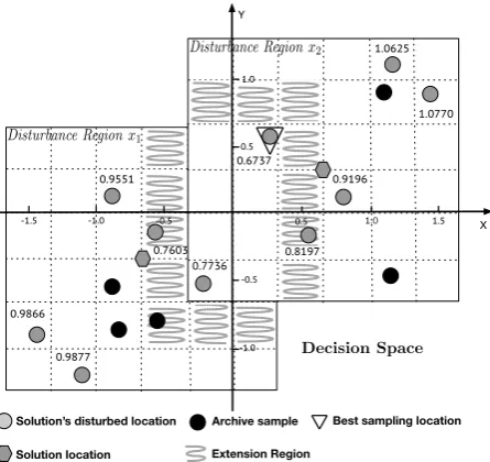
3.4 Using approximation region in WASA. . . 51
3.5 TheVP M S value computation in PMS. . . 52
3.6 1-D visualisation of original and effective fitness of the 5-D test prob-lems. Solid line: original fitness landscape. Dash line: effective fitness landscape. . . 56
3.7 Convergence comparison with respect to evaluations for various ap-proximation region parameters. . . 58
3.8 Convergence comparison with the evaluations for various sampling budget limits. . . 59
3.9 Comparison of approximation error reduction achieved various sam-pling strategies. . . 62
3.10 Convergence comparison of different sampling strategies with respect to evaluations. . . 63
3.11 Average approximation error comparison of different sampling strate-gies with respect to evaluations. . . 64
3.12 The baseline shape of the robust design problem. . . 67
4.1 An illustration of the clinical trials process. . . 77 4.2 An illustration of the decision tree structure. . . 81 4.3 Probability of observing a particular trajectory for the single drug
Acknowledgments
This thesis would not have been possible without the guidance and the help of
many people. First and foremost, I would like to express my deepest appreciation
to my supervisors, Dr. Nalˆan G¨ulpınar and Prof. J¨urgen Branke, for their support
and encouragement. It has been my honour to be one of their Ph.D. students.
They granted me the freedom to choose research directions and support me to
explore the unknown domains. Moreover, they have taught me, both consciously
and unconsciously, how to become a scientific researcher. I appreciate all their
contributions of time, effort and ideas to make my Ph.D. experience productive.
I would like to extend my sincere thanks to Prof. Bo Chen, Prof. Leroy
White, Prof. Steve Alpern and Dr. Arne K Strauss for their valuable advice during
the Ph.D. upgrade, annual review and completion review. I also have to thank the
members of my thesis defence committee, Dr. Xuan Vinh Doan, Professor Kevin
Glazebrook, and Dr. Vladimir Deineko for their helpful comments and suggestions.
My grateful thanks also go to my colleagues and friends: Bingqing Lan,
Folarin Oyebolu, Gongtai Wang, Mustafa Demirbilek, Wen Zhang, Ruini Qu for
their unstinting help, support and companionship.
Last but not the least, I would also like to say a heartfelt thank you to my
Declarations
I declare that any material contained in this thesis has not been submitted for a
degree to any other University. I further declare that one paper titled “Efficient
Solution Selection for Two-stage Stochastic Programs”, drawn from Chapter 2 of
this thesis, was co-authored with Nalˆan G¨ulpınar and J¨urgen Branke. It has been
accepted in European Journal of Operational Research. Furthermore, the paper
titled “New Sampling Strategies when Searching for Robust Solutions”, drawn from
Chapter 3 of this thesis, was co-authored with J¨urgen Branke and Nalˆan G¨ulpınar.
It has been accepted inIEEE Transactions on Evolutionary Computation. Finally,
the paper titled “An Adaptive Rollout Algorithm for Clinical Trial Scheduling and
Resource Allocation in Drug Development Under Uncertainty”, drawn from Chapter
4 of this thesis, was co-authored with Nalˆan G¨ulpınar and J¨urgen Branke.
Xin Fei
Abstract
This thesis focuses on a class of information collection problems in stochastic
op-timisation. Algorithms in this area often need to measure the performances of
several potential solutions, and use the collected information in their search for
high-performance solutions, but only have a limited budget for measuring. A
sim-ple approach that allocates simulation time equally over all potential solutions may
waste time in collecting additional data for the alternatives that can be quickly
identified as non-promising. Instead, algorithms should amend their measurement
strategy to iteratively examine the statistical evidences collected thus far and
fo-cus computational efforts on the most promising alternatives. This thesis develops
new efficient methods of collecting information to be used in stochastic optimisation
problems.
First, we investigate an efficient measurement strategy used for the solution
selection procedure of two-stage linear stochastic programs. In the solution selection
procedure, finite computational resources must be allocated among numerous
po-tential solutions to estimate their performances and identify the best solution. We
propose a two-stage sampling approach that exploits a Wasserstein-based screening
rule and an optimal computing budget allocation technique to improve the efficiency
of obtaining a high-quality solution. Numerical results show our method provides
good trade-offs between computational effort and solution performance.
Then, we address the information collection problems that are encountered
in the search for robust solutions. Specifically, we use an evolutionary strategy to
solve a class of simulation optimisation problems with computationally expensive
reduce the required number of evaluations. The main challenge in the application
of this method is determining the locations of additional samples drawn in each
generation to enrich the information in the archive and minimise the
approxima-tion error. We propose novel sampling strategies by using the Wasserstein metric
to estimate the possible benefit of a potential sample location on the
approxima-tion error. An empirical comparison with several previously proposed archive-based
sample approximation methods demonstrates the superiority of our approaches.
In the final part of this thesis, we propose an adaptive sampling strategy
for the rollout algorithm to solve the clinical trial scheduling and resource
alloca-tion problem under uncertainty. The proposed sampling strategy method exploits
the variance reduction technique of common random numbers and the empirical
Bernstein inequality in a statistical racing procedure, which can balance the
explo-ration and exploitation of the rollout algorithm. Moreover, we present an augmented
approach that utilises a heuristic-based grouping rule to enhance the simulation
ef-ficiency by breaking down the overall action selection problem into a selection
prob-lem involving small groups. The numerical results show that the proposed method
Chapter 1
Introduction and Background
1.1
Review of Efficient Information Collection
The diversity of real-world problems pose numerous challenges in information collec-tion that inspire new thoughts and research direccollec-tions. Many research communities have been formed to advance the state-of-the-art in measurement strategies and resolve practical information collection problems through theoretical and method-ological innovation. Powell and Ryzhov [2012] performed a comprehensive review of efficient information collection approaches and their applications. In the following, we review several studies that are more closely related to the works of this thesis.
expected value-of-information that myopically collects the sampling information to improve the decision-maker’s knowledge state. Chick and Inoue [2001] first proposed a two-stage sampling procedure in the principle of expected value-of-information. Chick et al. [2010] developed two sequential approaches that iteratively assign a small amount of samples to several or one designs per sampling stage. Frazier et al. [2009] later implemented this idea and proposed a so-called knowledge gradient method to handle the the R&S problem with correlated normal beliefs. Scott et al. [2011] extended the idea of knowledge gradient to account for continuous decision variables. For a comprehensive review on R&S methods, readers are referred to Branke et al. [2007].
assigns equal probabilities of obtaining evaluations to all candidate actions at the initial simulation stage and then sequentially increases the evaluation probabilities for promising candidate actions.
1.2
Structure of Thesis and Contributions
This thesis deals with some aspects related to efficient information collection in stochastic optimisation. Our focus is on sampling approaches that estimate the performance of potential solutions and guide algorithms towards the most promising solutions. The thesis structure and contributions are summarised as follows.
Chapter 2 studies the information collection problem that arises from the post-processing procedure of two-stage stochastic programs. The sampling-based stochastic programming model in the complex applications tends to be computa-tionally challenging. Thus, a reasonable sample size needs to be identified, and a group of approximate models can then be constructed using such a number of samples. These approximate models can produce a set of potential solutions. We consider the problem of distributing a finite computational budget among numerous potential solutions for identifying the best solution. We propose a two-stage mea-surement strategy: Firstly, we utilise a Wasserstein-based screening rule to remove a number of inferior solutions from the simulation. The key to the success of this screening rule is the quantitative stability of Wasserstein metric in stochastic pro-grams. We can infer an upper bound performance of potential solutions by using the Wasserstein distances between samples in the approximate models and those in the actual model. Secondly, we apply optimal computing budget allocation to de-termine the number of evaluations to be used for each solution. We conduct several numerical experiments to examine the performance of our approach. The numerical results indicate that the proposed approach outperforms existing approaches under relatively limited run times.
lies in determining the best locations of additional samples to complement existing simulation results and reduce the estimation error of mean performance. We use Wasserstein distance to estimate the possible benefit of a potential sample location on the estimation error, and propose new sampling strategies based on this metric to guide evolutionary algorithms towards the promising region of decision space. An empirical comparison with several previously proposed archive-based sample approximation methods demonstrates the superiority of our approaches.
In Chapter 4, we focus on drug development and propose an adaptive sam-pling strategy to support the rollout search process. Specifically, drug development is a process of testing the safety and efficacy of experimental drugs in a series of clinical trials, entrenched with a high uncertainty that an experimental drug will eventually get market approval. The profitability of drug development relies on effective strategic decision-making that comprises clinical trial scheduling and re-source allocation across multiple drug projects. In this work, the drug development problem is formulated as a discrete-time finite Markov decision process, and an adaptive rollout algorithm is introduced for the curse of dimensionality arisen in the stochastic dynamic program model. The proposed algorithm includes two innova-tions. First, a base policy is used to obtain optimistic estimates of future outcomes after taking a particular action at a state of the system. This policy utilises a rolling horizon optimisation model to identify a specific action to be taken at each state of the system and optimistically estimates the expected profit after a particular action is implemented. We prove that the optimistic policy follows a sequential consis-tency property and the performance of the rollout algorithm is at least as good as the optimistic policy. Second, an adaptive sampling approach is proposed to ef-ficiently identify the best action, which exploits the variance reduction technique of common random numbers and the empirical Bernstein inequality in a statistical racing procedure. Besides, we present an augmented adaptive sampling approach that utilises a heuristic-based grouping rule to enhance the simulation efficiency by breaking down the overall action selection problem into a selection problem involv-ing small groups. The proposed algorithms can provide competitive results within a reasonable computational time.
Chapter 2
Efficient Solution Selection for
Two-stage Stochastic Programs
2.1
Introduction
Real-life optimisation problems often involve uncertainties and require solutions that can handle such uncertainties in the modelling process. Techniques such as the two-stage linear stochastic programming with recourse (SPR) incorporate random data within the model formulation and determine a solution that satisfies the constraints and leads to the best expected objective function value for all possible scenarios. The development of SPR can be traced back to research conducted in the 1950s and 1960s, e.g., Beale [1955], Dantzig [1955] and Wets [1966]. The successful applications of SPR can be found in various sectors such as portfolio management [Dupaˇcov´a, 1999; Miller and Ruszczy´nski, 2011], energy planning [Beraldi et al., 2008; Zhou et al., 2013; Feng and Ryan, 2014], supply chain management [Joensson et al., 1993; Santoso et al., 2005; Dillon et al., 2017], and transportation planning [Cheung and Chen, 1998; Barbarosoˇglu and Arda, 2004; Liu et al., 2009].
con-struct approximate models, which provide potential solutions to the original SPR model. Monte-Carlo sampling as well as several variance reduction techniques such as quasi-Monte-Carlo sampling [Le¨ovey and R¨omisch, 2015; Heitsch et al., 2016], im-portance sampling [Parpas et al., 2015] and Latin hyper-cube sampling [Linderoth et al., 2006] can be utilised to generate such samples. Moreover, some authors sug-gested the generation of samples that should satisfy a specified criterion, such as probability distances [Pflug, 2001; Dupaˇcov´a et al., 2003] or moment discrepancies [Høyland et al., 2003; G¨ulpınar et al., 2004].
Once samples are generated, various optimisation algorithms can be used to solve the resulting SAA model. One approach is to utilise the simplex algorithm, which is conveniently implemented by modern optimisation solvers. Alternatively, some studies exploited the problem structure and proposed decomposition-based optimisation algorithms, for instance, see Dantzig and Wolfe [1960] and Van Slyke and Wets [1969]. Subsequently, numerous authors introduced advanced proce-dures such as the multi-cut approach [Birge and Louveaux, 1988], the trust region method [Linderoth and Wright, 2003], the regularised decomposition [Ruszczy´nski and ´Swietanowski, 1997] and the level bundle method [Wolf et al., 2014; van Ackooij et al., 2017] to improve the efficiency of utilising the decomposition principle. For a comprehensive review on decomposition approaches, the readers are referred to Rahmaniani et al. [2017].
decomposition-based method, is beneficial because the SAA user can implement a large sample size to strengthen the approximation of random data and obtain improved solutions within the same timeframe. Moreover, an effective solution se-lection method is also important because it can promptly determine the best option among a large group of potential solutions. However, only a limited number of studies is concerned with solution selection for the SPR problems.
Defourny et al. [2013] applied a brute-force approach that runs extensive simulations for each potential solution to identify a good policy in multi-stage linear stochastic programming. Instead of individually evaluating solution performance, Kleywegt et al. [2002] used a ranking and selection approach called indifference zone to determine a good solution in two-stage stochastic discrete optimisation. The indifference zone approach, which assigns simulation replications for each potential solution on the basis of performance statistics and guarantees the overall procedure at least a certain probability of selecting the best solution, was proposed by Nelson et al. [2001]. However, this approach is not an anytime algorithm, which means that a specified simulation rule (i.e. simulation replications for each potential solution) is followed to finish all requested simulations so that a probability guarantee is achieved. Also, this method is highly conservative and usually takes many more samples than necessary [Branke et al., 2007].
In the present study, we propose a solution selection method for the large-scale two-stage linear SPR problems that can deal with numerous potential solutions and return fairly efficient solutions within a finite computational budget. The con-tributions of this study are threefold.
• First, a Wasserstein-based screening (WS) approach is proposed to identify potentially promising solutions. We demonstrate that the worst-case perfor-mances of SAA solutions in the respective Wasserstein distance regions can be ranked by using the Wasserstein distance between the sampling measure used in the SAA model and the original probability measure. Solutions with small distance values have good worst-case performances and thus be classified as the most promising evaluated in the simulation.
withWS to improve the simulation efficiency.
• Third, we conduct several numerical experiments to analyse performance of
WS and theWS-OCBAapproaches. Results show thatWS achieves a satis-factory trade-off between the number of potential solutions in the promising group and the performance loss. The findings also indicate that WS-OCBA outperforms the existing approaches under relatively limited run times.
The remainder of this chapter is structured as follows. In Section 2.2 we provide a brief overview of two-stage stochastic programming and introduce the solution performance estimation procedure. Section 2.3 introduces the underlying principle of WS-OCBA. In Section 2.4, we explain the underlying principle of using Wasserstein distance in the solution screening. Section 2.5 discusses the estimation process of Wasserstein distance. Section 2.6 describes the proposed solution selection algorithm. In Section 2.7, we study the efficacy of our proposed strategies. Section 2.8 concludes this chapter by summarising our findings.
2.2
Sample Average Approximation for Two-stage
Lin-ear SPR
2.2.1 Two-stage Linear SPR Formulation
Let ξ ∈ Rµ be a random vector with finite second moments. Specifically, random
vector ξ is defined on the probability space (Ξ,B(Ξ),P), where Ξ is the sample
space, B(Ξ) is the Borel sigma algebra with respect to Ξ, and P :B(Ξ) → [0,1] is
the probability measure. Without loss of generality, a two-stage linear SPR problem with fixed recourse can be formulated as
min
x∈X f(x) = minx∈X c 0x+Z
Ξ
g(x, ξ)P(dξ) (2.1)
where c ∈ Rκ is a vector of constant parameters and X ⊂ Rκ represents a
non-empty convex feasible set. In addition, let g(x, ξ) denote the optimal value of the second-stage decision problem, formulated as follows:
g(x, ξ) = min
y∈Rι{
q0y|W y=H(ξ)−T(ξ)x, y≥0} (2.2)
where q ∈ Rι and W ∈ Rµ×ι are a fixed vector and a fixed matrix, respectively.
Moreover,T(ξ)∈Rµ×κ and H(ξ) ∈Rµ affinely depend on random vector ξ in this
We also make the following assumptions throughout this study:
A(1) Relatively complete recourse: For each tuple (ˆx, ξ), the corresponding
second-stage decision problem (2.2) is feasible.
A(2) Dual feasibility: The set {π|π0W ≤q}is not empty.
Assumption A(1) ensures the feasibility of the primal second-stage decision prob-lem. Assumption A(2) implies dual feasibility in the second-stage decision probprob-lem. Assumptions A(1) and A(2) represent necessary conditions for the stability result of the Wasserstein metric (for detailed information, see Dupaˇcov´a et al. [2003]) which will be used in our approach.
For the two-stage linear SPR problems, properties of the probability space majorly influence the computational burden. The problems, in the case of random data with continuous sample space, are rarely solvable because the resulting model formulation consists of an infinite number of second-stage decision variables and constraints. Moreover, the SPR problems might still suffer from computational intractability even when the probability distribution of random data is discrete. For instance, consider random data with 10 components, each of which follows a uniform distribution and can take 200 possible values. If we select one possible value for each component according to its distribution and then combine them as one sample, then the number of distinctive scenarios reaches 20010. Since the computational
complexity increases exponentially with the number of samples taken into account, the optimal solution is difficult to obtain [Shapiro and Homem-de Mello, 1998]. The SAA approach can be applied for identifying near-optimal solutions to the SPR problem.
2.2.2 The Near-optimal Solution and its Performance Estimator
Suppose that a group of samples ˆΞ ={ξˆm: m= 1, . . . , M} with respective
proba-bility values {Q( ˆξm) : m= 1, . . . , M} is generated from the random data, thereby
we can obtain the following approximate model,
min
x, y( ˆξm)
c0x+
M
X
m=1
Q( ˆξm)q0y( ˆξm)
s.t. x∈ X,
W y( ˆξm) =H( ˆξm)−T( ˆξm)x, m= 1, . . . , M,
y( ˆξm)≥0, m= 1, . . . , M.
The resulting solution is typically not the optimal solution for the original SPR model, so it is important to evaluate its performance in the original model.
Let ˆxandf(ˆx) denote a potential solution and its performance in the original model, respectively. Mak et al. [1999] suggested using Monte-Carlo estimation to infer the valuef(ˆx). Assume that we haveK i.i.d batches of samples with sizeNE
and equal probabilities; that is, ˜Ξk = {ξ˜nk : n = 1, . . . , NE}, for k = 1, . . . , K. We
can estimate a true solution performance for each batchkof samples by computing the optimal value ˆfNk
E(ˆx):
ˆ
fNkE(ˆx) = 1 NE
NE X
n=1
min
y( ˜ξk n)
c0xˆ+q0y( ˜ξnk)
s.t. W y( ˜ξnk) =H( ˜ξnk)−T( ˜ξnk)ˆx y( ˜ξnk)≥0.
(2.4)
By averaging over all optimal values ˆfNk
E(ˆx), for k= 1, . . . , K, we obtain an
estima-tor off(ˆx) as
J(ˆx) = 1 K
K
X
k=1
ˆ
fNkE(ˆx). (2.5)
Let σ2( ˆfNE(ˆx)) denote the unknown population variance of the optimal values of
SAA models with the first-stage decision ˆx and sample size NE. Mak et al. [1999]
demonstrated that J(ˆx) is an unbiased estimator and follows the Central Limit Theorem:
√
K
J(ˆx)−f(ˆx)
=√K
1 K K X k=1 ˆ
fNkE(ˆx)−f(ˆx)
→ N
0, σ2( ˆfNE(ˆx))
, (2.6)
when K → ∞. Note that N
0, σ2( ˆf
NE(ˆx))
is a Gaussian distribution with
vari-anceσ2( ˆfNE(ˆx)) and zero mean. Then, the population varianceσ
2( ˆf
NE(ˆx)) can be
estimated by using the following estimator as
V(ˆx) =
K
X
k=1
ˆ
fNkE(ˆx)− J(ˆx)2
K−1 . (2.7)
also beneficial for finding the optimal solution. In the following subsection, we will introduce the solution selection problem.
2.2.3 Solution Selection Under a Fixed Computing Budget
Suppose that a group of potential solutions is given and a simulation is required to select the best one as the final solution under the fixed computational budget. One of the challenges we might encounter is that the “best” solution based on Monte-Carlo estimation may not be really the best solution if insufficient information is available for analysing the solution performance. In this study, we model the solution selection process as a computing time allocation problem. Let {xˆλ : λ= 1, . . . ,Λ} denote a set of potential solutions. The performance of each solution ˆxλ is evaluated by Kλ
batch samples with sizeNE. The CPU time to compute each batch sample in (2.4) is
denoted byt(ˆxλ, NE). Let the batch numberKλ forλ= 1, . . . ,Λ represent unknown
decision variables. Moreover, we define ˆxs as the solution with best sample mean.
Given the total simulation budget Ttotal, the computing time allocation problem can be formulated as follows:
min
K1,K2,...,KΛ f(ˆx
s)
s.t.
Λ
X
λ=1
t(ˆxλ, NE)Kλ ≤Ttotal
ˆ
xs= arg min
1 Kλ
Kλ X
k=1
ˆ
fNkE(ˆx) :λ= 1, . . . ,Λ
Kλ∈N, λ= 1, . . . ,Λ.
(2.8)
It is challenging to solve the solution selection problem in the sense that its objective function represents true performance of potential solutions.
2.3
Optimal Computing Budget Allocation
quantifies the penalty due to wrong selection and is defined as follows:
E(OC) =E
f(ˆxs)−f(ˆxb)
=
Λ
X
λ=1, λ6=s
P rob(ˆxλ = ˆxb)
f(ˆxs)−f(ˆxλ)
, (2.9)
where P rob(ˆxλ = ˆxb) denotes the probability of solution ˆxλ being the true best solution ˆxb.
AsP rob(ˆxλ = ˆxb) is unknown in practice, He et al. [2007] proposed to use an upper bound approximation ofE(OC) that can be estimated during the simulation
procedure.
Theorem 2.1. Letφ(·) and Φ(·) be the probability density function (PDF) and
cu-mulative distribution function of standard normal distribution, respectively. More-over, Ks is the number of evaluated samples for the solution ˆxs and Kλ is the number of evaluated samples for solution ˆxλ. The upper bound approximation of expected opportunity cost (abbreviated as AEOC) is presented as follows:
E(OC)≤AEOC=
Λ
X
λ=1,λ6=s
Vs,λ×φ(zs,λ) +δs,λ×Φ(−zs,λ)
(2.10)
where Vs,λ = V(ˆx
s)
Ks + V
(ˆxλ)
Kλ , δs,λ = J(ˆxs)− J(ˆxλ) and zs,λ =
−δs,λ √
Vs,λ
. Note that
V(ˆxλ) and V(ˆxs) are the estimation variances of solution ˆxλ and ˆxs, which can be computed by Equation (2.7).
Proof. He et al. [2007] provided an upper bound approximation for the probability P rob(ˆxλ = ˆxb) as follows,
P rob(ˆxλ = ˆxb)≤P rob
f(ˆxλ)< f(ˆxs)
. (2.11)
Hence, we can obtain
E(OC)≤
Λ
X
λ=1,λ6=s
P rob
f(ˆxλ)< f(ˆxs)
f(ˆxs)−f(ˆxλ)
=
Λ
X
λ=1,λ6=s
Z +∞
0
t ηs,λ(t) dt= AEOC,
(2.12)
whereηs,λdenotes the PDF of random valueN
f(ˆxs)−f(ˆxλ),Vs,λ
He et al. [2007], we can apply the integration by parts method to compute (2.12) as follows,
Z +∞
0
t ηs,λ(t) dt=Vs,λφ(zs,λ) +δs,λΦ(−zs,λ). (2.13)
Given a finite computing budget, we aim to allocate the simulation budget to se-quentially minimise the upper bound of expected opportunity cost. If we evaluate one additional sample for the solution ˆxλ, then the upper bound of expected oppor-tunity cost will change to
\
AEOCλ=
Λ
X
λ0=1,λ06=s
Z ∞
0
x ηs,λ0,λ dx, λ= 1, . . . ,Λ, (2.14)
whereηs,λ0,λ is the PDF of the normally distributed random variable and defined as
N
f(ˆxs)−f(ˆxλ),KV(ˆsx+1s) +V
(ˆxλ0)
Kλ0
, if ˆxλ= ˆxs
N
f(ˆxs)−f(ˆxλ),VK(ˆxss)+ V
(ˆxλ0)
Kλ0+1
, if ˆxλ= ˆxλ0
N
f(ˆxs)−f(ˆxλ),V(ˆxs) Ks +V
(ˆxλ0)
Kλ0
, if ˆxλ6= ˆxs and ˆxλ 6= ˆxλ0 .
The above integration can be computed by using (2.10). Then, the possible reduc-tion of AEOC can be computed as,
Yλ= AEOC−AEOC\λ≥0. (2.15)
Notice that the valueYλ forλ= 1, . . . ,Λ is always non-negative because theOCBA
procedure aims to greedily reduce E(OC) by sampling the performances of SAA
solutions. In other words, Yλ represents the estimated improvement on E(OC)
when evaluating the performance of SAA solution ˆxλ. If the improvement for a
SAA solution is negative, then we will stop the sampling procedure. Next, the sample would be assigned to the solution that leads to the maximum reduction of AEOC, i.e.,
λ∗ = arg max{Yλ: λ= 1, . . . ,Λ}. (2.16)
potential solutions. For instance, if the limited computing budget runs out during the initial estimation of Algorithm 2, then some solutions will not be evaluated. If the best solution is one of those ignored, then it is not possible to correctly identify the best solution. Moreover, the solution selection method is challenging when the computing budget is insufficient in the sequential decision process because the initial estimation has taken a large proportion of the computing budget. Then insufficient estimation might mislead our choice of the final solution.
Algorithm 2.1: TheOCBA Procedure
input :potential solutions: {xˆλ : λ= 1, . . . ,Λ};
size of sampleNE in the performance estimation;
number of samplesK0 evaluated in the initial estimation.
output:best solution based on the simulation results.
1 whilesimulation budget is available do
2 Step 1: Initial Estimation;
3 forλ= 1, . . . ,Λ do
4 evaluate the performance of solution ˆxλ using K0 samples; 5 compute the performance statistics of solution ˆxλ using (2.6) and
(2.7);
6 select the current best solution ˆxs;
7 Step 2: Sequential Decision Process;
8 forλ= 1, . . . ,Λ do
9 compute the expected opportunity cost reduction Yλ as in (2.10) and (2.14);
10 findλ∗ = argmax{Yλ, λ= 1, . . . ,Λ};
11 simulate one additional sample for solution ˆxλ∗ and update its statistics;
12 select the current best solution ˆxs.
2.4
Wasserstein-based Solution Screening
extensive simulation. A similar paradigm called “ordinal transformation” is used in a simulation optimisation study [Xu et al., 2016], wherein the authors considered the simulation output on a user-defined low-fidelity model as the low-cost measure for each potential solution. The potential solutions were clustered according to low-fidelity simulation results and the extensive simulation was applied to select the best solution cluster.
The Wasserstein distance metric, a kind of statistical metric for quantifying the dissimilarity between two probability measures, is the key component of WS
method. The definition of Wasserstein metric can be found in Appendix A. This metric has been widely applied in stochastic programming. One application is sce-nario reduction wherein the Wasserstein distance is used as the quality indicator of samples in the approximate model. Given a fixed number of samples used in the approximate model, some authors proposed heuristics to select the “best” sam-ples with minimum distance. For example, Dupaˇcov´a et al. [2003] presented two myopic scenario reduction heuristics for two-stage SPR, namely, forward selection and backward reduction. Furthermore, Heitsch and R¨omisch [2009] extended these heuristics for multi-stage SPR. In another application, the Wasserstein distance was used to define an ambiguity set for stochastic programs with distributional uncer-tainty [Mohajerin Esfahani and Kuhn, 2017]. In addition, the Wasserstein distance was applied to reduce the optimality gap estimator bias, and this application bene-fits testing the optimality of a given solution [Stockbridge and Bayraksan, 2013]. In this study, we use the Wasserstein distance metric to roughly rank the performance of potential solutions.
Before stating the main result, we first introduce the stability result of stochastic programming.
Theorem 2.2. Assume that the solution sets of original model and SAA model are
singleton. Letx∗ and ˆxdenote the unique solutions of the original model and SAA model, respectively. Moreover, let P be the original probability measure, and Q
represent the sampling measure of a SAA model. The difference between measures
P and Q is quantified by the Wasserstein distance W(P,Q). Under assumptions
A(1) and A(2), there exit constantsτ >0 andε >0 such that
kx∗−xˆk2 ≤
2τ
Proof. For details, see the proof of Theorem 1 introduced by Dupaˇcov´a et al. [2003].
Theorem 2.2 utilises two constants τ and ε to establish the Lipschitz-like prop-erty of SAA solutions with respect to changes in the probability measure. Next, we will show the relationship between the solution performance and the corresponding Wasserstein distance.
Theorem 2.3. Under assumptions A(1) and A(2), the performance difference
be-tween solutionsx∗ and ˆx satisfies the following inequality:
f(ˆx)≤f(x∗) +h|Lxˆ|,τ Wˆ (P,Q)Ii, (2.17)
whereLˆx=E[πˆx(ξ)T(ξ)] +c withπxˆ(ξ) = argmax{π0[H(ξ)−T(ξ)ˆx] : π0W ≤q},
ˆ
τ = 2ετ is a positive coefficient, andI ∈Rκ is the all one vector.
Proof. Consider the two-stage SPR problem given in (2.1). Under assumptions A(1) and A(2), the Proposition 2.3 introduced by Shapiro et al. [2009] proved that, if functiong(ˆx, ξ) for ˆx∈ X, ξ ∈Ξ is finite, then the objective function f(·) will be sub-differentiable at the point ˆx. LetLxˆ denote one of sub-gradients for solution ˆx.
The following sub-gradient inequality holds,
f(x∗)≥f(ˆx) +hLxˆ, x∗−xˆi. (2.18)
Shapiro et al. [2009] showed that the sub-gradientLxˆ of a two-stage SPR problem
can be calculated as
Lxˆ =E[π0xˆ(ξ)T(ξ)] +c,
whereπxˆ(ξ) represent a vector of dual decisions associated with constraints of the second-stage problem (2.2). It is computed as follows,
πˆx(ξ) = arg max
π {π
0[H(ξ)−T(ξ)ˆx] : π0W ≤q}.
By substituting the sub-gradient and re-arranging both sides of inequality (2.18), we obtain
f(ˆx)−f(x∗)≤ −hE[πx0ˆ(ξ)T(ξ)] +c, x∗−xˆi. (2.19)
minimisa-tion problem. Therefore, we can obtain
|f(ˆx)−f(x∗)| ≤ h|E[πx0ˆ(ξ)T(ξ)] +c|,|x∗−xˆ|i. (2.20)
Using Theorem 2.2, the distance between solutions x∗ and ˆx is upper bounded by the Wasserstein distanceW(P,Q) as follows,
kx∗−xˆk2 =
v u u t
κ
X
κ0=1
(x∗κ0−xˆκ0)2 ≤ 2τ
ε W(P,Q)≤τ Wˆ (P,Q) (2.21)
where ˆτ = 2ετ is a positive coefficient. For each element of solutions x∗ and ˆx, we can write
ˆ
τ W(P,Q)≥ v u u t
κ
X
κ0=1
(x∗κ0−xˆκ0)2≥
q
(x∗κ0−xˆκ0)2 =|x∗
κ0−xˆκ0|, κ0 = 1, . . . , κ. (2.22) Therefore,|x∗−xˆ|can be approximated by using the Wasserstein distance,W(P,Q),
as follows,
|x∗−xˆ| ≤τ Wˆ (P,Q)I. (2.23)
By combining inequality (2.23) with (2.19), we obtain (2.17).
Theorem 2.3 implies that performance of potential solution ˆx is bounded by the sub-gradient Lxˆ and the Wasserstein distance W(P,Q). The potential solution ˆx
becomes the optimal solutionx∗for the actual problem if either probability measures
Qand Pare identical or the sub-gradient at ˆx becomes zero.
As mentioned before, the Wasserstein distance W(P,Q) can be efficiently
estimated using Monte-Carlo estimation; however, the calculation of sub-gradients
Lxˆ for two-stage liner SPRs is computationally expensive. Next, we introduce the
worst-case solution performance in the Wasserstein-bounded region. We will use this performance measure in the solution screening procedure.
Definition 2.1: Worst-case Solution Performance in the Wasserstein Re-gion. Let Γ ˆx(Q) represent a set possessing sub-gradients of all feasible solutions
be determined as follows:
Gw(ˆx) = max L0∈Γ ˆx(
Q)
f(x∗) + L0
,τ Wˆ (P,Q)I . (2.24)
Notice that Gw(ˆx) is defined as a maximisation problem with respect to the
sub-gradient value L0. The next theorem states the applicability of the Wasserstein distance in sequencing the worst-case performance of potential solutions.
Theorem 2.4. Consider a set of potential solutions {xλ : λ = 1, . . . ,Λ} with
respective Wasserstein distances{W(P,Qλ) : λ= 1, . . . ,Λ}. Let [λ] denote theλ-th
potential solution in the increasing sequence of Wasserstein distances as
W(P,Q[1])≤W(P,Q[2])≤ · · · ≤W(P,Q[Λ]). (2.25)
Then, the worst-case solution performances of these solutions satisfy,
Gw(ˆx[1])≤ Gw(ˆx[2])≤ · · · ≤ Gw(ˆx[Λ]). (2.26)
Proof. Assume that the Wasserstein distances satisfy the sequence as in (2.25). Since the inequality (2.23) can be written for all potential solutions ˆxλ, we can construct the same relationship as in sequence of
n
x:|x−x∗| ≤τ Wˆ (P,Q[1])I o
⊆nx:|x−x∗| ≤τ Wˆ (P,Q[2])I o
⊆ · · · ⊆nx:|x−x∗| ≤τ Wˆ (P,Q[Λ])I o
.
(2.27)
Hence, the feasibility set of all sub-gradients at approximate potential solutions holds the sequence of
Γ ˆx[1](Q)⊆Γ ˆx[2](Q)⊆ · · · ⊆Γ ˆx[Λ](Q). (2.28)
Theorem 2.4 indicates that the sequence of Wasserstein distances for SAA solu-tions encapsulates the trend of the worst-case solution performances. We should note that the rank of actual solution performances in general does not follow the sequence of Wasserstein distances. Therefore, when the solution screening is applied according to the sequence of Wasserstein distances, a performance loss that is caused by eliminating the best solution might arise. We describe the performance loss as follows.
Definition 2.2: Performance Loss. Let {xˆλ0
: λ0 = 1, . . . ,ΛP} denote a set of promising solutions obtained from a specific screening procedure. If the com-puting budget is restricted on those promising solutions, then the performance loss (P L) due to screening out the best solution can be computed as
P L= min{f(ˆxλ0) : λ0 = 1, . . . ,ΛP} −min{f(ˆxλ) : λ= 1, . . . ,Λ}. (2.29) IfP L= 0, then the promising group contains the best solution. Otherwise, P L is always greater than zero. The value P L reflects the quality of the promis-ing group; thus, havpromis-ing a screenpromis-ing procedure that has a performance guarantee is desirable. Next, we prove that the proposed screening approach provides an upper bound for the performance loss.
Theorem 2.5. Assume that for a set of potential solutions {xˆλ : λ = 1, . . . ,Λ},
the corresponding set of Wasserstein distances{W(P,Qλ) : λ= 1, . . . ,Λ}possesses
an increasing sequence of distance values. In other words, the following inequalities hold:
W(P,Q[1])≤W(P,Q[2])≤ · · · ≤W(P,Q[Λ]). (2.30)
Then, the Wasserstein-based screening provides the following upper bound for the performance loss:
P L≤ Gw(ˆx[1])−min{f(ˆxλ) : λ= 1, . . . ,Λ}. (2.31)
Proof. From (2.17) and (2.24), we can write the following inequality for each promis-ing solution
Hence, from the definition of performance loss, it follows:
min{f(ˆxλ0) : λ0= 1, . . . ,ΛP} ≤min{Gw(ˆxλ0) : λ0 = 1, . . . ,ΛP}. (2.33) This yields
P L= min{f(ˆxλ0) : λ0= 1, . . . ,ΛP} −min{f(ˆxλ) : λ= 1, . . . ,Λ}
≤min{Gw(ˆxλ0) : λ0 = 1, . . . ,ΛP} −min{f(ˆxλ) : λ= 1, . . . ,Λ}. (2.34) Clearly, selecting a promising subgroup of solutions out of the top ΛP of the lowest Wasserstein distances (using Theorem 2.3) provides
P L≤ Gw(ˆx[1])−min{f(ˆxλ) : λ= 1, . . . ,Λ}. (2.35) So by combining with (2.34), we find that (2.31) holds.
Theorem 2.5 implies that the Wasserstein-based screening provides a fixed upper bound for the performance loss even without performing any simulation. The tight-ness of the bound depends on the stability result of the Wasserstein distance.
2.5
Wasserstein Distance Estimation
In this section, we introduce a method of estimating Wasserstein distance in the two-stage linear SPR problems. Let N denote the number of samples for original probability measure, andM be the number of samples in the sampling measure. Ac-cording to the definition of Wasserstein distance in Appendix A, the transportation problem involvesN×M decision variables andN+M+N×M linear constraints. If the value of N is very large or even infinite, then the corresponding computa-tional complexity will be intractable. In the context, we can replace the probability measure P with a group of sampling measures, and take the average Wasserstein
distance between random measures and probability measureQ as the estimator of
W(P,Q). The following Lemma states that the bias of such an estimator is bounded.
Lemma 2.1. Let Pi for i = 1, . . . ,I denote the sampling measure induced by
NW realisations generated from the probability measureP. If we use the estimator
ˆ
W(P,Q) = 1 I
I
X
i=1
to infer the Wasserstein distance valueW(P,Q), then its bias satisfies the following
inequality,
W(P,Q)−Wˆ(P,Q) ≤
1
I
I
X
i=1
W(Pi,P). (2.36)
Proof. Since the Wasserstein distance is a metric, it satisfies the reverse triangle inequality:
|W(P,Q)−W(Pi,Q)| ≤W(Pi,P). (2.37)
Next, we can compute the sum of inequalities (2.37) over allPi fori∈ I as follows;
−
I
X
i=1
W(Pi,P)≤ I ×W(P,Q)−
I
X
i=1
W(Pi,Q)≤
I
X
i=1
W(Pi,P). (2.38)
By dividing both sides of the above inequality by I, we obtain inequality (2.36).
Lemma 2.1 states that the absolute value of estimation bias is bounded by the aver-age Wasserstein distance. We can increase the sample size of the sampling measure to minimise the fluctuation of bias. The main benefit of using Lemma 2.1 is to re-duce the computational burden due to the large sample number. We can now solve a group of relatively small optimisation problems to infer the actual Wasserstein distance W(P,Q). Each “small” optimisation problem only has NW ×M decision
variables and NW +M +NW ×M constraints. The overall Wasserstein distance
estimation procedure is described in Algorithm 2.2.
Algorithm 2.2: Wasserstein Distance Estimation Procedure
input :number of sampling measuresI;
number of samples in each sampling measureNW.
output:estimated Wasserstein distance value ˆW(P,Q).
1 generateI groups of i.i.dNW realisations from probability measure P;
2 fori= 1, . . . ,I do
3 compute the Wasserstein distanceW(Pi,Q) using (A.1);
4 end
5 Wˆ(P,Q)← 1
I I X
i=1
2.6
The Proposed Two-stage Selection Approach
We propose a two-stage method that combines the Wasserstein-based screening method with the optimal computing budget allocation. Algorithm 2.3 describes integration of the solution screening approach intoOCBA. The Wasserstein-based solution screening method selects potential solutions that are then more closely examined using OCBA. The solution screening procedure takes a proportion of the computing budget. Thus, it is necessary to properly allot the computing bud-get among different procedures; namely, solution screening, initial estimation, and sequential allocation. We now highlight some rules for a practical application of Algorithm 2.3.
Algorithm 2.3: TheWS-OCBAProcedure
input :candidate solutions: {xˆλ: λ= 1,· · · ,Λ};
size of sampleNE in the performance estimation;
number of samplesI with sizeNW in Wasserstein distance;
number of promising solutions: ΛP;
number of samplesK0 evaluated in the initial estimation.
output: best solution based on the simulation results.
1 forλ= 1,· · ·,Λdo
2 run Algorithm 2.2 for solutionxλ to estimate the corresponding Wasserstein distance;
3 rank and select the top ΛP candidate solutions according to their Wasserstein distances;
4 whilecomputing budget is available do
5 implement the evaluation procedure as in Algorithm 2.1.
As shown in Algorithm 2.3, the Wasserstein-based solution screening selects candidates that are then more closely examined using the OCBA algorithm. The solution screening procedure takes a proportion of computing budget. Thus, it is necessary to properly allot the computing budget for the procedures, namely, solution screening, initial estimation, and sequential decision. We now highlight the rules for the practical application of Algorithm 2.3.
Table 2.1: Complexity of benchmark problems
Problem Instances D/C Dim N S Optimal Values
1ststage 2ndstage
LandS 4/2 12/7 3 1×10⁶ 225.620±0.020
Retail 7/0 70/22 7 1×10¹¹ 154.410±0.770
20term 64/3 764/124 40 1.1×10¹² 254298.572±38.743
SSN 89/1 706/175 86 1.1×1070 9.840
±0.100
• A large sample size is preferred for the Wasserstein distance estimation be-cause it helps to reduce potential estimation bias; however, the computational cost of the Wasserstein distance estimation should be controlled to a certain level, which aims to secure sufficient computing budget in OCBA. The rule of thumb is that, for a single solution, the computational cost of the Wasser-stein distance estimation should be smaller than that of the initial estimation in Algorithm 2.1, because the Wasserstein distance estimation is designed to be a fast simulator. Otherwise, it might be wise to use the initial simulation results for eliminating the inferior actions.
• The number of potential solutions to be run for simulation (i.e., promising solutions) is determined by the computing budget to be allocated forOCBA. We should guarantee to have sufficient computing budget for Step 2 of Algo-rithm 2.1. Otherwise, the insufficient simulation may lead to selection errors.
2.7
Numerical Experiments
2.7.1 Overview of Test Instances
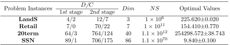
In this section, we describe four benchmark problem instances to be used for the numerical experiments. Table 2.1 presents complexity of these instances in terms of number of decision variables (D), constraints (C), dimension of uncertainties (Dim), number of scenarios (N S) as well as the optimal values (mean ± standard error). The corresponding problem descriptions are briefly summarised as below:
• LandSis an electricity planning problem [Louveaux and Smeers, 1988]. The
first-stage decisions are concerned with an allocation of four power terminals, and the second-stage decisions are related to allocating the power supply to various residential areas.
problem involving multiple retailers and one supplier. The objective is to design the optimal replenishment policy for each retailer.
• 20term, adopted from Linderoth et al. [2006], is a large-scale vehicle
man-agement problem. The first-stage decisions find the vehicle locations at the beginning of the plan, and the second-stage decisions optimise the fleet trans-portation plan on the basis of the initial vehicle locations.
• SSN[Sen et al., 1994] aims to design an optimal telecommunication network that can minimise the number of lost demands. In view of randomness of the communication demand in the network, the bandwidth between destination and origin nodes must be sufficiently large to satisfy the customer demand. Otherwise, that demand will be lost.
All test instances are minimisation problems, which are written in SMPS format and publicly available online 1. This study implements an SMPS parser that is based on the Julia programming language and the COIN-OR linear program solver. All numerical experiments are computed on a machine with i7-6700K CPU and 32GB memory.
2.7.2 Wasserstein Distance-based Screening with Various Numbers of Promising Solutions
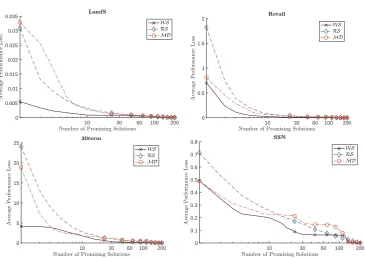
We adopt the following benchmark strategies to compare withWS:
• Random screening (RS): a fixed number of solutions is randomly selected from the potential solutions.
• Moment discrepancy (MD): a fixed number of solutions is selected according to the total discrepancy of the first four statistical moments (mean, variance, skewness and Kurtosis) between measuresP and Q.
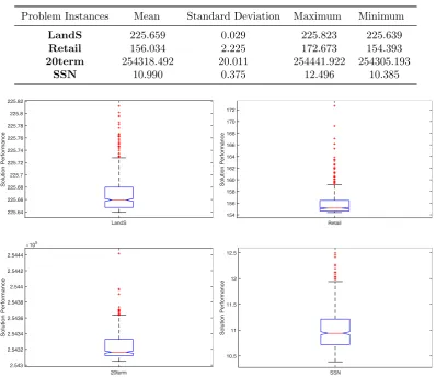
The experimental settings are as follows. We implement SAA with 200 sam-ples to generate 200 approximate solutions for each test instance. Table 2.2 shows the statistical description of those approximate solutions. Figure 2.1 graphically illustrates performances of the potential solutions in terms of the mean, range and confidence intervals. We apply three strategies to select various numbers (from 1 to 200) of solutions and compute the corresponding performance loss (as discussed in Section 2.4). The performance of each solution is evaluated with 30 groups of
1
http://pages.cs.wisc.edu/~swright/stochastic/sampling/ and http://plato.asu.edu/
Table 2.2: Statistical description of potential solutions.
Problem Instances Mean Standard Deviation Maximum Minimum
LandS 225.659 0.029 225.823 225.639
Retail 156.034 2.225 172.673 154.393
20term 254318.492 20.011 254441.922 254305.193
SSN 10.990 0.375 12.496 10.385
Retail 154 156 158 160 162 164 166 168 170 172 Solution Performance SSN 10.5 11 11.5 12 12.5 Solution Performance LandS 225.64 225.66 225.68 225.7 225.72 225.74 225.76 225.78 225.8 225.82 Solution Performance 20term 2.543 2.5432 2.5434 2.5436 2.5438 2.544 2.5442 2.5444 Solution Performance 105
Figure 2.1: Box plots providing the mean (horizontal line in box), range (vertical lines extending from box), and 95% confidence intervals (vertical extent of box) for the performances of candidate solutions.
500,000 samples. For WS, the solution’s Wasserstein distance is estimated using four samples with a size of 1,000.
10 30 60 100 200 0
0.005 0.01 0.015 0.02 0.025 0.03 0.035
10 30 60 100 200
0 0.5 1 1.5 2
10 30 60 100 200
0 5 10 15 20 25
10 30 60 100 200
[image:40.595.139.505.100.358.2]0 0.1 0.2 0.3 0.4 0.5 0.6 0.7 0.8
Figure 2.2: Comparison of average performance losses obtained by RS and WS
using various numbers of promising solutions.
performance loss changes with the problem structure. For example, more solutions need to be included in the simulation procedure for 20term and SSN than LandS and Retail.
2.7.3 Average Performance Comparison with Benchmark Algorithms
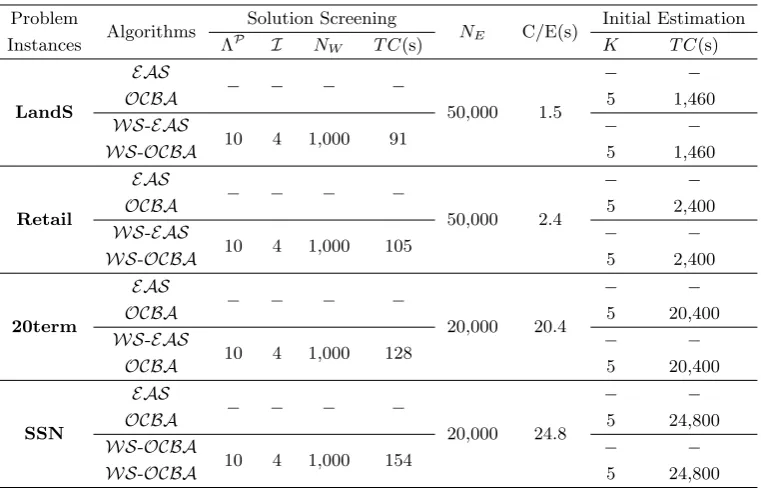
We also conduct numerical experiments to study the performance of the solution selection algorithm in terms of the CPU time. The performance of WS-OCBA is compared with that of the following approaches.
• OCBAis the standardOCBA algorithm as described in Algorithm 2.1 .
• EAS uses equal allocation and selection algorithm, which sequentially allocates the same number of simulations to each candidate solution and selects the current best solution based on the simulation results.
• WS-EAS employsEAS with the proposed Wasserstein-based solution screen-ing procedure.
This procedure is repeated 100 times to examine the average performance of each algorithm. The detailed experimental settings are listed in Table 2.3. Figure 2.3 presents the convergence comparisons over 100 runs in terms of CPU time and average solution performance. The computational costs of solution screening for the
[image:41.595.132.513.221.468.2]WS-based algorithms are included in the comparison results.
Table 2.3: Experimental settings.
Problem
Algorithms Solution Screening NE C/E(s)
Initial Estimation
Instances ΛP I NW T C(s) K T C(s)
LandS
EAS
− − − −
50,000 1.5
− −
OCBA 5 1,460
WS-EAS
10 4 1,000 91 − −
WS-OCBA 5 1,460
Retail
EAS
− − − −
50,000 2.4
− −
OCBA 5 2,400
WS-EAS
10 4 1,000 105 − −
WS-OCBA 5 2,400
20term
EAS
− − − −
20,000 20.4
− −
OCBA 5 20,400
WS-EAS
10 4 1,000 128 − −
OCBA 5 20,400
SSN
EAS
− − − −
20,000 24.8
− −
OCBA 5 24,800
WS-OCBA
10 4 1,000 154 − −
WS-OCBA 5 24,800
ΛP: number of promising solution;I: number of samples for Wasserstein estimation; NW : sample size for Wasserstein estimation;T C: total CPU time;
NE: sample size for performance evaluation; C/E: CPU time of each evaluation
K: number of samples used in the initial estimation.
0 500 1000 1500 2000 2500 3000 225.64
225.642 225.644 225.646 225.648 225.65 225.652 225.654
0 500 1000 1500 2000 2500 3000
154.4 154.45 154.5 154.55 154.6 154.65
0 1500 3000 4500 6000 7500
2.54328 2.54329 2.5433 2.54331 2.54332 2.54333 2.54334 2.54335 2.54336 10
5
0 1500 3000 4500 6000 7500
[image:42.595.123.517.103.399.2]10.4 10.45 10.5 10.55 10.6 10.65 10.7 10.75
Figure 2.3: Convergence comparison with respect to CPU time.
However,OCBAperforms worse than any of theWS-based algorithms on all test instances, indicating that WS enhances performance of the solution selection algorithm for the case of numerous potential solutions. ForWS-OCBA, the compu-tational cost for initial estimation is greatly reduced. We observe thatWS-OCBA
Table 2.4: Average solution performance of the selected subset (mean ±std. err).
Problem CPU Algorithms
Instances Time (s) EAS OCBA WS-EAS WS-OCBA
LandS
1,000 225.648±0.002 225.647±0.001 225.648±0.002 225.647±0.001
2,000 225.648±0.001 225.645±0.001 225.644±0.001 225.643±0.001
3,000 225.647±0.001 225.645±0.001 225.643±0.001 225.641±0.001
Retail
1,000 154.556±0.013 154.545±0.017 154.499±0.009 154.449±0.003
2,000 154.545±0.012 154.506±0.008 154.490±0.009 154.431±0.001
3,000 154.554±0.013 154.490±0.006 154.479±0.003 154.408±0.001
20term
2,500 254334.892±1.041 254334.267±1.050 254333.018±0.894 254331.562±0.835
5,000 254334.172±0.952 254334.797±0.948 254332.134±0.707 254330.358±0.665
7,500 254335.117±0.936 254335.062±0.931 254331.255±0.792 254328.726±0.706
SSN
2,500 10.654±0.015 10.645±0.014 10.595±0.014 10.543±0.012
5,000 10.589±0.015 10.586±0.016 10.546±0.011 10.430±0.009
7,500 10.553±0.013 10.553±0.014 10.534±0.011 10.461±0.008
We display the performance of the solutions obtained from the various algo-rithms averaged over 100 repetitions in Table 2.4. Best results and those statistically not different from best are highlighted in bold. The results confirm the importance of adopting solution screening in the selection procedure for numerous potential so-lutions. TheWS-based algorithms significantly outperform the others in all bench-mark problems, although all algorithms display similar performance in LandS and 20terms when the CPU time is 1,000s. Moreover, we find thatWS-OCBAperforms better thanWS-EAS due to its advanced computing budget allocation scheme.
2.8
Conclusions
Chapter 3
Efficient Sampling Strategies
when Searching for Robust
Solutions
3.1
Introduction
Given its ubiquity in many real-world problems, optimisation under uncertainty has gained increasing attention. Uncertainty may originate from various sources, such as imprecise model parameters or fluctuations in environmental variables. In the presence of uncertainty, it is often desirable to find a solution that is robust in the sense of performing well under a range of possible scenarios [Beyer and Sendhoff, 2007]. More specifically, our paper considers searching for robust solutions in the sense of high expected performance, given a distribution of disturbances to the decision variables. This is a typical scenario for example in manufacturing, where the actually manufactured products may differ from the design specification due to manufacturing tolerances.
Evolutionary algorithms (EAs) have been applied to solve various optimi-sation problems that involve uncertainties, see Jin and Branke [2005] for a survey. There are also different concepts related to robustness, including optimising the worst-case performance [Ong et al., 2006], robust optimisation over time [Fu et al., 2015], and active robustness [Salomon et al., 2016]. The most widely researched robustness concept however, and the concept we consider in this chapter, is to op-timise a solution’s expected fitness (often called effective fitness in the literature) over the possible disturbances [Beyer and Sendhoff, 2007].
in practice, and two sampling methods can be distinguished. Implicitsampling refers to the idea that because EAs are population-based, an over-evaluated individual due to a favourable disturbance can be counterbalanced by an under-evaluated neigh-bouring individual, and so simply increasing the population size should help guiding the EA in the right direction, e.g. see Rattray and Shapiro [1998] and Beyer and Sendhoff [2006]. In fact, as shown in Tsutsui and Ghosh [1997], under the assump-tion of infinite populaassump-tion size and fitness-proporassump-tional selecassump-tion, evaluating each solution at a single disturbed sample location instead of its actual location is equiv-alent to optimising the expected fitness directly. Beyer and Sendhoff [2006] proposed to increase the population size whenever the algorithm gets stalled. Explicit sam-pling, on the other hand, evaluates each individual multiple times and estimates its fitness as the average of the sampled evaluations. Obviously, while averaging over multiple evaluations increases the estimator accuracy, it is computationally rather expensive. A recent analytical study on the efficiency (progress rate) of implicit as well as explicit sampling-based evolution strategies can be found in Beyer and Sendhoff [2017].
Because of the large computational cost of sampling in case of expensive fitness functions, numerous studies have focused on allocating a limited sampling budget to improve the estimation accuracy, allowing to reduce the number of sam-ples needed without degrading the performance of the EA. One possible approach for estimating effective fitness is to apply quadrature rules or variance reduction techniques, e.g. see Branke et al. [2001]; Di Pietro et al. [2004]; Huang and Du [2006] and Lee et al. [2009]. Some authors observed that allocating samples in a manner that increases the probability of correct selection is more important than the accuracy of estimation [Stagge, 1998; Branke and Schmidt, 2003].
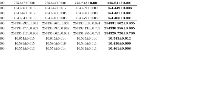
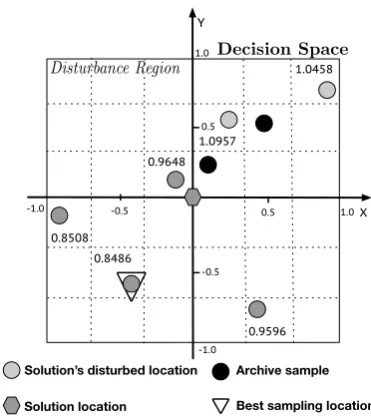
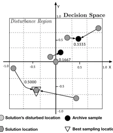
Another approach, called archive sample approximation (ASA), stores all past evaluations in a memory and uses this information to improve expected fitness estimates in future generations (for further information, refer to Branke et al. [2001] and Kruisselbrink et al. [2010]). ASA can also be combined with the above sampling allocation methods to further enhance the accuracy of approximation. We have recently proposed an improved ASA method that uses the Wasserstein distance metric (a probability distance that quantifies the dissimilarity between two statistical objects) to identify the sample that is likely to provide the most valuable additional information to complement the knowledge available in the memory [Branke and Fei, 2016].
Fei [2016] is one of many possible approaches in the WASA framework. Here, a new sampling strategy based on WASA is presented, which improves the performance in three ways:
1. A heuristic that considers what sample might provide the most valuable infor-mation forallindividuals in the populationsimultaneously, thereby enhancing the performance of the final solution and accelerating the convergence of the EA toward a high-performance solution;
2. Introducing the concept of an approximation region that could improve the performance of the sampling strategy when few samples exist; and
3. Proposing a sample budget mechanism to adjust the sampling budget in the WASA framework.
This chapter is structured as follows. Section 3.2 provides a brief overview of existing archive sample approximation methods. We then present our new ap-proaches to allocating samples in Section 3.3. These apap-proaches are evaluated empir-ically using benchmark problems, and their performances are compared with other approaches in Section 3.4. This chapter concludes with a summary.
3.2
Archive Sample Approximation
The problem of searching for robust solutions can be defined as follows. Consider an objective functionf :x→R with design variablesx∈Rm. The noise is defined on
the probability space (Ξ,B(Ξ),P) where Ξ = Qm
i [`i, ui] is a sample space, B(Ξ) is
the Borelσ-algebra on Ξ andP is the probability measure onB(Ξ). For a particular solutionx, location zx is random under this noisy environment, which is defined as:
zx =x+ξ, ξ ∈Ξ. (3.1)
We then define the induced probability space for zx as (Dx,B(Dx),Px), where Dx
is the disturbance region as the set covering all possible locations as a result of disturbing solutionx defined by:
Dx= m
Y
i=1
[xi+`i, xi+ui]; (3.2)
andPx is the probability measure defined so that, for φ∈ B(Dx),