Self tuning of PI speed controller gains using fuzzy logic controller

Self-Tuning of PI Speed Controller Gains

Using Fuzzy Logic Controller

Mutasim Nour (Corresponding author)

School Electrical and Electronic Engineering, University of Nottingham Malaysia campus

Jalan Broga, 43500 Semenyih, Salangor, Malaysia

Tel: 60-3-8924-8122 E-mail: mutasim.nour@nottingham.edu.my

Omrane Bouketir & Ch’ng Eng Yong

School Electrical and Electronic Engineering, University of Nottingham Malaysia campus

Jalan Broga, 43500 Semenyih, Salangor, Malaysia

Tel: 60-3-8924-8159 E-mail: omrane@nottingham.edu.my

Abstract

The role of proportional-integral (PI) controller and proportional-integral-derivative (PID) controller as a speed controller for a Permanent Magnet Synchronous Motor (PMSM) in high performance drive system is still vital although new control techniques such as vector control theory that is more effective -but complex- is available. However, PI controller is slow in adapting to speed changes, load disturbances and parameters variations without continuous tuning of its gains. Conventional approach to these issues is to tune the gains manually by observing the output of the system. The tuning must be made on-line and automatic in order to avoid tedious task in manual control. Hence, an on-line self-tuning scheme using fuzzy logic controller (FLC) is proposed in this paper. The performance of the developed proposed controller is tested through a wide range of speeds as well as with load and parameters variations through simulation using MATLAB/SIMULINK. It is found that the proposed 25 rules FLC with adaptive input and output scaling factors enhances the performance of the system especially at high load inertia. The simulation results show that the developed controller can well adapt to speed changes as well as sudden speed reduction besides fast recovery from load torque and parameters variation and these show remarkable improvement compared to conventional PI controller performance.

Keywords: Adaptive Control, Fuzzy Logic, PI Controller, Speed Controller

1. Introduction

In process control today, more than 95% of the control loops are of PID type, most loops are actually PI control (Karl, 2002), (Gupta,2002). For example, it is used to regulate the speed of a motor, pressure of a chamber and heat of an oven. The popularity of PI control can be attributed to its simplicity (in terms of design and from the point of view of parameter tuning) and to its good performance in a wide range of operating conditions (Leandro et al., 2000). The design of PI or PID controller is simple as the computations of the proportional gain, integral gain and derivative gain by means of second-order method or Ziegler-Nichols method are well-defined. However, the normal PI controllers present as a disadvantage the need of retuning whenever the processes are subjected to some kind of disturbance or when processes present complexities (non-linearities) (Karasakal, 2005).

fixed gains calculated is good when the system is running with rated speed and rated conditions. Often, when running a system there will be a lot of speed changes, load disturbances and parameter variations (Mutasim & Shirren, 2006). Hence, the fixed gains of the PI controller will not be able to perform the compensation role for such conditions without re-tuning its parameters. This collaboration is practical as most of the industrial system that are using conventional controller can insert a FLC to their control system for optimization purposes without changing much of the system topology and scrapping the conventional controller.

In recent years, there has been an increasing interest in developing alternative methodologies for designing industrial PI controllers such as auto-tuning, self-tuning, pattern recognition, fuzzy logic, neural network and genetic algorithm. For fuzzy logic alone, many investigations and research on different types of adaptive fuzzy PI and PID controllers have been reported in (Hoang, 1995), (Onur et al., 2003), (Kouzi, et al., 2003) and (Mutasim et al., 2005). In general, fuzzy logic PI controller design can be classified into two major categories according to the way of their construction: Either the gains of the conventional PI controller are tuned on-line in according to the knowledge base and fuzzy inference, and then the conventional PI controller generates the control signal or a typical FLC is constructed as a set of heuristic control rules, or the control signal is directly deduced from the knowledge base and the fuzzy inference (Mudi & Pal., 1999).

In this paper, a two-input and two-output FLC is used to tune the PI gains of permanent magnet synchronous motor (PMSM) controller. The tuning is made on-line to compensate for any load disturbances, speed changes and system parameter variations. The inputs for the FLC are error (E) and change of error (CE) while the outputs are change in proportional gain (CKp) and change in the integral gain (CKi). The outputs of the FLC are used to tune the respective gains of the PI controller to optimum values. Since the FLC tunes the existing PI controller gains on-line, it is described as the self-tuning of PI gains using fuzzy logic controller. Throughout the paper, this controller is described as fuzzy-PI controller for simplicity.

2. Controller Design Methodology

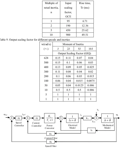
A typical control structure of a PMSM is shown in Figure 1 (Krishnan, 2001). As the current time constant is much smaller than the mechanical time constant, a change in current loop is very much faster compared to a change in speed loop. Hence, current loop can be represented by simply a gain or constant. This can ease the design of speed controller as the control structure is reduced to second-order system and Figure 1 is simplified to Figure 2.

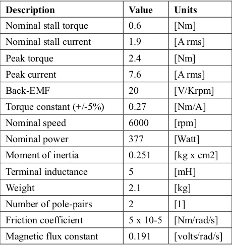
Based on A 380W PMSM parameters given in Table 1, satisfactory values for proportional gain (Kp) and integral gain

(Ki) were determined using Ziegler-Nichols method (Kp = 0.2 and Ki= 2.1). These values were used as a starting point

for the fuzzy-PI controller to update the gains accordingly based on the error and change of error. The starting points of gains are chosen to be at half rated speed to make the tuning of gains to be equivalent for lowest speed and highest speed.

2.1 Extraction of the FLC Rules

An experiment to study the effect of rise time (Tr), maximum overshoot (Mp) and steady-state error (SSE) when varying

Kp and Ki was conducted. The results of the experiment were used to develop 25-rules for the FLC of Kp and Ki. The

followed procedure is outlined below.

The effects on the rise time (Tr), maximum overshoot (Mp) and steady state error (SSE) of the response were observed

when varying Ki while fixing Kp at 0.2 and varying Kp while fixing Ki at 2.1. Table 2 records these effects. The values

of Kp and Ki are obtained through the design of PI Controller as stated above. The reference speed is set to be from 300

to -300 rad/s that is about 50 % of the rated speed with full-load (FL). The results in Table 2 are used to create Table 3 that shows the effect of varying Kp and Ki. This table is created in such a way that the magnitude of the effects on Tr, Mp

and SSE are determined when the gains of Kp and Ki are varied.

2.2 Membership Functions Selection

The design of FLC is based on Table 3 in deciding when to manipulate Kp and Ki based on the response of the system.

For example, when steady-state error is big, gains of Kp and Ki should be increased and vice versa. Error Ek can be

represented by steady-state error (SSE) while change in error CEk can be approximated by rise time (Tr) since:

T E E

CE ₌ 2 − 1 ₍₁₎

where T is sampling time, E2 is current error and E1 is previous error. The normalised speed error Ek and the normalised

change of error CEk can be calculated from:

k ref

k k ref k E

ω ϖ

ω −

k ref

k k k

E E CE

ω− −1

= (3)

where ωref k is reference speed (rad/s), ωk is measured speed (rad/s) and Ek-1 is previous normalised error. Ek and CEk are

the two inputs to the FLC to calculate the change of proportional gain CKp and change of integral gain CKi which will

be summed together to form the new input current command iq for the control of PMSM. Notice that, equation (2) and

(3) are normalised by the reference speed at every instance. This is to scale the value of Ek and CEk down to the range

of -1 to 1 as the range of the universe of discourse for the membership functions of FLC is selected to be from -1 to 1 as will be seen later in the following sections.

The effective gain for proportional control (TKp) and integral gain (TKi) can be calculated as:

p p

p K TCK

TK = + (4)

i i

i K TCK

TK = + (5)

where TCKp is sum of changes in proportional gain, TCKi is sum of changes in integral gain, Kp is the initial

proportional gain set and Kiis the initial integral gain set.

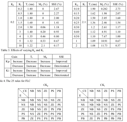
The behaviour of implementing the rules in Table 4 is identical to the often used rule base designed with a two-dimensional phase plane which has 49 rules (Yanan & Collin, 2003). Series of tests were performed to choose the most suitable membership function (MF). A comparison between the performance of four MFs types were conducted and revealed that the assymmetrical Bell-shaped performed better than symmetrical Bell-shaped, asymmetrical triangle-shaped and symmetrical triangle-shaped MFs. Therefore, assymmetrical Bell shaped MFs were employed in this work.

3. Tuning Mechanism

3.1 GCE Tuning

The FLC previously designed can be improved further by tuning one input of the FLC. This input gain (GCE) that needs to be tuned is the change of error (CE) input for the FLC. GCE is tuned with respect to speed changes. Different speed response has different optimum values of GCE as shown in Table 5. By using these values, the response of the system is tested to be significantly better in term of rise time. Hence, data from Table 5 is used to form an on-line tuning mechanism for different speed applied. The method chosen is called the look-up table method or gain scheduling. In this method, different GCE values from -628 to 628 rad/s are written into a programme and the other in between values are calculated based on interpolation method. Interpolation is a process for estimating values that lie between known data points. The high maximum overshoot output responses due to the change of moment of inertia can also be overcome by changing the values of GCE as shown in Table 6.

To minimize the maximum overshoot, the price for it is slower rise time. In other words, there is a need to compromise between rise time and maximum overshoot. In Table 6, the values of GCE are optimised so that the maximum overshoot is eliminated but the rise time for the system raised quite significant as can be seen in Table 7. The main reason for doing this is to avoid the system to be damaged by high overshoot. The simulation model in this stage is modified by including the gain scheduling process. The slow rise time due to the increased inertia cannot be tolerated in high performance drive system. Hence, further improvement for the rise time is done next.

3.2 GCE and GIQ (I/O Gains) Tuning

It is found that by tuning of GIQ as a function of inertia and speed and fixing GCE tuning results in smoother and faster response for certain speeds. In addition, high overshoot and slow response as a result of increased inertia can also be overcome. Hence the output control signal is scaled up or down accordingly by GIQ as a function of speed and moment of inertia. From Table 9, it is obvious that as inertia increases, GIQ decreases. This is to make sure the FLC updates the Kp and Ki with a smaller value to avoid overshoot because the overshoot increases when inertia increases as discovered

previously.

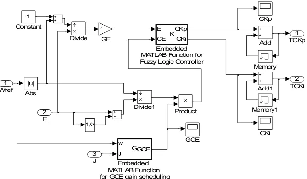
When only the GIQ is changed, the recovery of speed from load changes become slower. To overcome this problem, GIQ needs to be tuned as a function of load as well. When load occurs, the output gain must be increased to ensure the response recovers from load changes faster. It is observed that for all speed, the recovery from load changes is fast by using a fix GIQ of 1. The final stage of the developed controllers can be seen clearly from the simple block diagram shown in Figure 3.

4. Results and Discussion

performance of the fixed-gain FLC are presented in this section. The simulation block diagram model in Simulink is given in Figure 4.

4.1 Fixed Gains PI Controller

Graphs in Figure 5 shows a collection of results obtained from the simulation model that uses a fixed PI controller gains as a speed controller. The gains of the parameters are set based on half rated conditions at + 300 rad/s. At these conditions, the PI controller plays its role well. However, when the speed changes to the rated speed which is 628 rad/s or any other speed, high overshoot and high steady-state error (SSE) occurs. This is because the fixed gains of the controller cannot adapt to speed changes well.

4.2 Fixed-Gain FLC

Figure 6 shows the performance of the FLC at first stage of development that is with fixed input and output gains. The performance of this control is good throughout a wide range of speed with zero SSE and fast rise time. The only drawback of this FLC is high overshoot at increased inertia. High overshoot occurs when the inertia is varied as can be seen from Figure 6 (a). This occurs because FLC tune the gains of PI controller to very high value due to the slow response of the system and by the time the response reaches the reference speed, FLC failed to decrease the high value of gains instantly and this causes the overshoot. However, the response tends to settle down to zero SSE after a short time but the overshoot for the response of 10 J is considered very high and is not acceptable in most of the applications. Although, it is very unlikely that 10 J is going to occur in real-time but effort in minimizing the overshoot is made as can be seen in next part of the results. As for the case of PI controller, the effect of varying the stator resistance and the stator inductance on the response of the system is not significant as shown in Figure 6 (b) and (c). Figure 6 (d) shows that the FLC can adapt to small speed reduction well at J and acceptable response with some overshoot is obtained at 2 J. These two responses follow the small speed reduction very fast with zero SSE.

Fast recovery from load changes to zero SSE can be seen in the magnified figures in Figure 7 whether at forward transient or reverse transient. The dip as a result of load is very small and is hardly visible if it is not magnified. These show that the developed FLC can adapt to load changes very well.

4.3 Tuned-Gains FLC

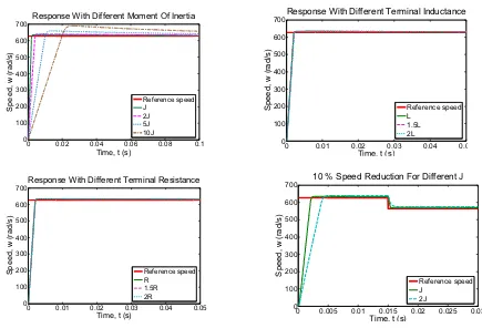
Results in this part shows the final developed FLC with I/O Gains tuning responses. The results seen below are proven to be very satisfactory especially for different moment of inertia as in Figure 8 (a). Smooth and considerably fast response with negligible overshoot is obtained for different values of J. As expected, response with different resistance and inductance does not have significant changes as it is the case for other controllers as previously discussed. Figure 8 (d) shows the controller can adapt to small speed reduction at nominal J as well as increased J well. The response time for the increased inertia is longer as expected.

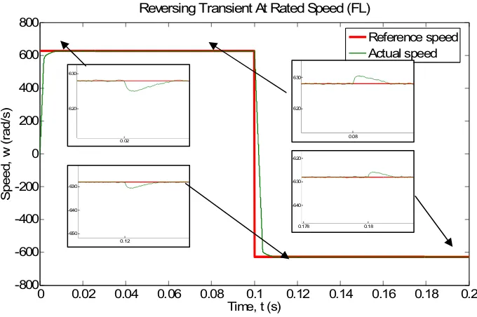
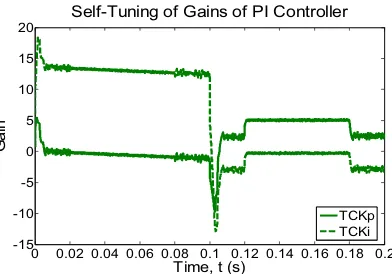
Figure 9 shows that the proposed controller can improve the transient response and further smooth the speed response compared to results obtained with the FLC with fixed input and output gains as shown in Figure 7. Besides, very fast recovery from load changes can also be obtained at forward transient where the dip as a result of load disturbance is very small an not clearly visible even though when it is magnified. For the reverse transient case, the recovery from load changes is considerably fast. The variations in the gains depicted in Figure 10. Initially, it can be seen that both the gains increased to high value at starting point because the error at this point is very big. As the response reaching zero SSE, the gains are seen to decrease to avoid excessive gains that will cause overshoot and leads to deterioration of stability.

When FL is applied and removed at 0.02 s and 0.08 s respectively, the gains at this point are enough to compensate for the load disturbances as no increment of gains are seen. During reverse transient at 0.1 s, the gains are decreased abruptly for the motor to rotate in another direction and then settle down back when reaching zero SSE at the reverse transient. When FL is applied again at 0.12 s, it can be seen that the gains increased for load recovery. When FL is removed at 0.18 s, the gains are seen to decreased back to the original value before FL is applied.

The control signal iq as a result from the self-tuning controller gains and the electromagnetic responses are shown in

Figure 11. Initially, very high current is needed to start the motor to overcome friction and inertia. When the motor starts to rotate, lesser current is needed. However, the current increased to approximately 1.9 A (rms) when FL is applied at 0.02 s and 0.12 s. This current is the rated current of the motor.

5. Conclusion

smoothness. The developed controller is proven to be robust as it was applied to control the motor speed at different speeds and parameters variation. Since, PI controller is still widely used in industry; the developed FLC can be applied to the available PI controller for optimization purposes once the implementation is carried out successfully. The developed control algorithm has been proven successfully in simulation and the next step is to be implemented in hardware using “Intelligent Motor Drive Module Development (IMDMD15)”.

References

Gupta, S. (2002). Elements of Control Systems: Prentice Hall, Upper Saddle River, NJ.

Hoang, L-H. (1995). An Adaptive Fuzzy Controller for Permanent Magnet AC Servo Drives, in Conf. Rec. of IEEE IAS Annual Meeting: 104-110.

Karasakal, O., Yesil, E., Guzelkaya, M., Eksin, I. (2005). Implementation of a New Self-Tuning Fuzzy PID Controller on PLC. Turk Journal of Electrical Engineering, 13(2):277-286.

Karl, J. A. (2002). Control System Design. Lecture Notes for ME155A. Department of Mechanical & Environmental Engineering University of California Santa Barbara. (Chapter 6). [Online] Available http://www.cds.caltech.edu/~murray/courses/cds101/fa02/caltech/astrom.html (June 9, 2007).

Kouzi, K., Mokrani, L. & Naït-Saïd, M.S. (2003). A Fuzzy Logic Controller with Fuzzy Adapted Gains Based on Indirect Vector Control for Induction Motor Drive. Journal of Electrical Engineering. 3:49-54.

Krishnan, R. (2001). Electric Motor Drives, Modeling, Analysis and Control: Prentice Hall (Chapter 9).

Leandro dos Santos, C., Otacilio da Mota, A., & Antonio Augusto Rodrigues, C. (2000). Design and Tuning of Intelligent and Self-Tuning PID Controllers. In The 5th Online World Conference on Soft Computing In Industrial Applications, Helsinki. IEEE Finland Section: 213-220.

MATLAB Manual, The MathWorks, Inc. 1984-1999.

Mudi, R. K. & Pal N. R. (1999). A Robust Self-tuning Scheme for PI- and PD-type Fuzzy Controllers. IEEE Trans. Fuzzy Systems, 7 (1): 2-16.

Mutasim, N. & Shirren, T. (2006). Adaptive Fuzzy Logic Speed Controller with Torque Adapted Gains for PMSM Drives. Journal of Engineering Science and Technology, 1(1): 59-75.

Mutasim, N., Aris, I., Mariun, N., Mohibullah, S.M. (2005). Hybrid Model Reference Adaptive Speed Control for Vector Controlled PMSM Drive. IEEE Sixth International Conference on Power Electronics and Drive Systems (PEDS05), Kuala Lumpur, Malaysia.

Onur, K., Engin, Y., Mujded G., Ibrahim, E. (2003). An Implementation of Peak Observer Based Self-Tuning Fuzzy PID-Type Controller on PLC. 3rd International Conf. on Electrical and Electronics Engineering, 2003, Turkey: 474-497. Yanan, Z. & Emmanuel G. C. (2003). Fuzzy PI Control Design for an Industrial Weigh Belt Feeder. IEEE Trans. Fuzzy Systems, 11(3), 311-319.

Table 1. PMSM parameters

Description Value Units

Nominal stall torque 0.6 [Nm]

Nominal stall current 1.9 [A rms]

Peak torque 2.4 [Nm]

Peak current 7.6 [A rms]

Back-EMF 20 [V/Krpm]

Torque constant (+/-5%) 0.27 [Nm/A]

Nominal speed 6000 [rpm]

Nominal power 377 [Watt]

Moment of inertia 0.251 [kg x cm2]

Terminal inductance 5 [mH]

Weight 2.1 [kg]

Number of pole-pairs 2 [1]

Friction coefficient 5 x 10-5 [Nm/rad/s]

Table 2. Transient and steady-state response for speed from 300 to -300 rad/s at FL

Table 4. The 25 rules for FLC

Where: NB: Negative Big; NS: Negative Small; ZE: Zero Error; PS: Positive Small; PB: Positive Big.

Table 5. GCE at different speed and load conditions

w(rad/s) (+-) Input scaling factor for CE (GCE)

628 95

500 75

400 60

300 45

200 35

100 20

50 15

10 6

5 4

1 1.5 Kp Ki Tr (ms) Mp (%) SSE (%)

0.2

0.2 1.80 0 2.67

0.5 1.80 0 2.27

1.0 1.80 0 2.00

1.5 1.60 0 1.41

2.0 1.50 0.06 1.18

3 1.40 0.20 0.93

4 1.35 0.46 0.80

5 1.32 0.33 0.67

10 1.22 2.1 0.17

Kp Ki Tr(ms) Mp (%) SSE (%)

0.10

2.1

1.90 0.282 2.73

0.15 1.62 1.98 2.07

0.20 1.50 2.05 1.60

0.25 1.36 2.46 1.54

0.30 1.2 2.61 1.17

0.40 1.12 4.91 1.10

0.50 1.10 7.67 1.00

1 1.09 10.91 0.67

2 1.08 11.73 0.37

Table 3. Effects of varying Kp and Ki

Gain Tr Mp SSE

Kp Increase Decrease Increase Improved

Decrease Increase Decrease Deteriorated

Ki Increase Decrease Increase Improved

Decrease Increase Decrease Deteriorated

CE E

NB NS ZE PS PB

NB NB NS NS NS ZE

NS NB NS NS ZE PS

ZE NB NS ZE PS PB

PS NS ZE PS PS PB

PB ZE PS PS PS PB

CE E

NB NS ZE PS PB

NB NB NB NB NS ZE

NS NB NB NS ZE PS

ZE NB NS ZE PS PB

PS NS ZE PS PB PB

PB ZE PS PB PB PB

Table 6. GCE at different moments of inertia

Multiple of rated inertia, n

1 2 5 10

Input scaling factor, GCE

95 190 450 900

Table 7. Rise time of the system with different moments of inertia and GCE

Multiple of rated inertia,

n

Input scaling factor,

GCE

Rise time, Tr (ms)

1 95 6.71

2 190 12.36

5 450 25.62

10 900 49.51

Table 9. Output scaling factor for different speeds and inertias

w(rad/s) Moment of Inertia

(+-) J 2J 5J 10J

Output Scaling Factor (GIQ)

628 0.15 0.11 0.07 0.04

500 0.15 0.1 0.06 0.03

400 0.13 0.09 0.05 0.025

300 0.11 0.08 0.04 0.02

200 0.1 0.06 0.03 0.015

100 0.06 0.04 0.015 0.0075

50 0.05 0.04 0.0125 0.006

10 0.5 0.5 0.5 0.006

5 1 1 1 1

1 1 1 1 1

Figure 1. Typical Control Structure for PMSM

PI

Speed Controller

PI

Current

Controller Power

Converter

KT

B Js+

1

Mechanical

Model

Hc

Current Filter

λF

Hs

Speed Filter

Electrical

Model

Tem

ωref

Σ Σ Σ Σ

iqref iq

R Ls+

1 1

+

s s T

K ωe

Figure 2. Simplified Control Structure of PMSM

B

Js

+

1

Mechanical Model

ωref

Σ ωr

s

K

K

p

+

PI Controller

Figure 3. Simulation Block Diagram of the Proposed System

2 TCKi

1 TCKp

1/z

Product Memory1

Memory 1

GE

GCE w

J GGCE

Embedded MATLAB Function for GCE gain scheduling

E

CE CKp

CKi K

Embedded MATLAB Function for Fuzzy Logic Controller

Divide1 Divide

1

Constant

CKp

CKi Add1

Add

|u|

Abs

3 J 2

E 1

Wref

0 0.02 0.04 0.06 0.08 0.1 0 100 200 300 400 500 600 700

Time, t (s)

Sp ee d, w (r a d/ s )

Response With Different Moment Of Inertia

Reference speed J

2J 5J 10J

0 0.01 0.02 0.03 0.04 0.0

0 100 200 300 400 500 600 700

Time, t (s)

Sp ee d, w (r a d /s )

Response With Different Terminal Inductance

Reference speed L

1.5L 2L

0 0.01 0.02 0.03 0.04 0.05

0 100 200 300 400 500 600 700

Time, t (s)

Sp ee d, w (r a d/ s )

Response With Different Terminal Resistance

Reference speed R

1.5R 2R

0 0.005 0.01 0.015 0.02 0.025 0.03

0 100 200 300 400 500 600 700

Time, t (s)

Sp ee d, w (r ad /s )

10 % Speed Reduction For Different J

Reference speed J

2J

Figure 5. Response of the System Using Fixed Gains PI Controller

0 0.02 0.04 0.06 0.08 0.1

0 200 400 600 800 1000 1200

Time, t (s)

Spee d, w ( ra d /s )

Response With Different Moment of Inertia

Reference speed J 2J 5J 10J (a)

0 0.01 0.02 0.03 0.04 0.05

0 100 200 300 400 500 600 700

Time, t (s)

Spee d, w ( ra d /s )

Response With Different Terminal Resistance

Reference speed R

1.5R 2R

(b)

0 0.01 0.02 0.03 0.04 0.05

0 100 200 300 400 500 600 700

Time. t (s)

Spee d, w ( ra d /s )

Response With Different Terminal Inductance

Reference speed L

1.5L 2L

(c)

0 0.01 0.02 0.03 0.04 0.05

0 100 200 300 400 500 600 700 800

Time, t (s)

Speed

, w (

rad/

s)

10 % Speed Reduction For Different J

Reference speed J

2J

Figure 7. Reversing Transient at Full-load Using Fixed I/O Gains FLC

Figure 8. Response of the System Using I/O Gains-Tuning FLC

0 0.02 0.04 0.06 0.08 0.1 0.12 0.14 0.16 0.18 0.2 -800 -600 -400 -200 0 200 400 600 800

Reversing Transient At Rated Speed (FL)

Time, t (s)

S p ee d, w ( rad /s ) Reference speed Actual speed 0.02 620 630 0.08 620 630 p( ) 0.12 -650 -640 -630 0.178 0.18 -640 -630 -620

0 0.02 0.04 0.06 0.08 0.1

0 100 200 300 400 500 600 700 Time, t(s) S p eed, w ( rad/ s)

Response With Different Moment Of Inertia

Reference speed J 2J 5J 10J (a)

0 0.01 0.02 0.03 0.04 0.05

0 100 200 300 400 500 600 700

Time, t (s)

Sp eed, w ( rad/ s)

Response With Different Terminal Resistance

Reference speed R

1.5R 2R

(b)

0 0.01 0.02 0.03 0.04 0.05

0 100 200 300 400 500 600 700

Time, t (s)

Sp eed, w ( ra d /s)

Response With Different Terminal Inductance

Reference speed L

1.5L 2L

(c)

0 0.01 0.02 0.03 0.04 0.05

0 100 200 300 400 500 600 700

Time, t (s)

Sp ee d, w ( ra d /s )

10 % Speed Reduction For Different J

Reference speed J

2J

0 0.05 0.1 0.15 0.2 -10

-7.5 -5 -2.5 0 2.5 5 7.5 10

Control Current Vs Time

Time, t (s)

C

u

rren

t,

i

q

(A

)

0 0.02 0.04 0.06 0.08 0.1 0.12 0.14 0.16 0.18 0.2

-5 -4 -3 -2 -1 0 1 2 3 4 5

Electromagnetic Torque Vs Time

Time, t (s)

T

o

rque,

T

e

m

(

N

m

)

Figure 11. The Current and the Electromagnetic Torque Responses

0 0.02 0.04 0.06 0.08 0.1 0.12 0.14 0.16 0.18 0.2

-15 -10 -5 0 5 10 15 20

Time, t (s)

Ga

in

Self-Tuning of Gains of PI Controller

TCKp TCKi

Figure 10. Self-tuning of TCKp and TCKi

0 0.02 0.04 0.06 0.08 0.1 0.12 0.14 0.16 0.18 0.2

-800 -600 -400 -200 0 200 400 600 800

Time, t (s)

S

p

e

ed,

w

(r

ad/

s

)

Reversing Transient at Rated Condition (FL)

Reference speed Actual speed

0.02 620

630

0.08 620

630

0.116 0.118 0.12 0.122 -680

-670 -660 -650 -640 -630 -620 -610

0.18 0.182 0.184 -680

-670 -660 -650 -640 -630 -620 -610