Reference layer artefact subtraction (RLAS): a novel method of minimizing EEG artefacts during simultaneous fMRI

(1)

Reference layer artefact subtraction (RLAS): A novel method of

minimizing EEG artefacts during simultaneous fMRI

☆

Muhammad E.H. Chowdhury, Karen J. Mullinger, Paul Glover, Richard Bowtell

⁎

Sir Peter Mansﬁeld Magnetic Resonance Centre, School of Physics & Astronomy, University of Nottingham, Nottingham NG7 2RD, UK

a b s t r a c t

a r t i c l e i n f o

Article history:

Accepted 16 August 2013 Available online 28 August 2013

Keywords:

Simultaneous EEG–fMRI Artefact correction Motion artefact Gradient artefact Pulse artefact Artefact removal

Large artefacts compromise EEG data quality during simultaneous fMRI. These artefact voltages pose heavy demands on the bandwidth and dynamic range of EEG amplifiers and mean that even small fractional variations in the artefact voltages give rise to significant residual artefacts after average artefact subtraction. Any intrinsic reduction in the magnitude of the artefacts would be highly advantageous, allowing data with a higher band-width to be acquired without amplifier saturation, as well as reducing the residual artefacts that can easily swamp signals from brain activity measured using current methods. Since these problems currently limit the utility of simultaneous EEG–fMRI, new approaches for reducing the magnitude and variability of the artefacts are required. One such approach is the use of an EEG cap that incorporates electrodes embedded in a reference layer that has similar conductivity to tissue and is electrically isolated from the scalp. With this arrangement, the artefact voltages produced on the reference layer leads by time-varyingfield gradients, cardiac pulsation and subject movement are similar to those induced in the scalp leads, but neuronal signals are not detected in the reference layer. Taking the difference of the voltages in the reference and scalp channels will therefore reduce the artefacts, without affecting sensitivity to neuronal signals. Here, we test this approach by using a simple experimental realisation of the reference layer to investigate the artefacts induced on the leads attached to the reference layer and scalp and to evaluate the degree of artefact attenuation that can be achieved via reference layer artefact subtraction (RLAS). Through a series of experiments on phantoms and human subjects, we show that RLAS significantly reduces the gradient (GA), pulse (PA) and motion (MA) artefacts, while allowing accurate recording of neuronal signals. The results indicate that RLAS generally outperforms AAS when motion is present in the removal of the GA and PA, while the combination of AAS and RLAS always produces higher artefact attenuation than AAS. Additionally, we demonstrate that RLAS greatly attenuates the unpredictable and highly variable MAs that are very hard to remove using post-processing methods.

Introduction

The combination of electroencephalography (EEG) with functional magnetic resonance imaging (fMRI) has opened up many new avenues of investigation in functional neuroimaging. In particular, the simulta-neous recording of EEG and fMRI data provides an ideal combination of the excellent spatial resolution of fMRI (Yacoub et al., 2001) with the millisecond temporal resolution of EEG (Amor et al., 2005). Simulta-neous EEG–fMRI has already been shown to have great potential for providing new understanding of the relationship between spontaneous or evoked electrical activity and the haemodynamic response in the

human brain (Debener et al., 2005; Goldman et al., 2002; Laufs et al., 2003). The technique has also found an important clinical application in epilepsy, by spatially localizing the interictal discharges measured in EEG (Gotman et al., 2004; Hamandi et al., 2004) through correlation with the haemodynamic responses measured in fMRI. However, to real-ise the full bene_ﬁt of simultaneous EEG_–fMRI, it is important to ensure that the data acquired when the two techniques are implemented si-multaneously are not signiﬁcantly compromised in quality compared with data produced in separate recordings.

Simultaneous recording of EEG and fMRI data is technically chal-lenging because the magnetic fields necessary for fMRI generate several artefacts in the EEG data (Allen et al., 1998, 2000), which are much larger in magnitude than the neuronal activity of interest. The largest artefact is produced by the temporally varying magnetic field gradients used in fMRI. These magneticfield gradients induce voltages in the conducting tissues of the human body and the wires of the EEG recording system by the process of electromagnetic induction (Yan et al., 2009). The resulting gradient artefact(GA) can be 10_–100 mV in magnitude compared with typical EEG signal

☆ This is an open-access article distributed under the terms of the Creative Commons Attribution License, which permits unrestricted use, distribution, and reproduction in any medium, provided the original author and source are credited.

⁎ Corresponding author at: Sir Peter Mansﬁeld Magnetic Resonance Centre, School of Physics & Astronomy, University of Nottingham, Nottingham NG7 2RD, UK. Fax: +44 115 9515166.

E-mail address:[email protected](R. Bowtell).

Contents lists available atScienceDirect

NeuroImage

(2)

amplitudes of less than 100μV. The induced voltages are dependent on the position of the head and EEG cap with respect to the applied magnetic_field gradients and have a temporal form that depends on the temporal derivative of the applied gradient waveforms (Allen et al., 2000). Since the gradients used for fMRI are highly consistent across repeated executions of the imaging sequence, the GA has a reproducible form, as long as the positions of the head or EEG cap do not change during acquisition. A second artefact is caused by movement linked to the subject's cardiac cycle. The exact aetiology of thispulse artefact(PA) is not well understood, but potential causes include the Hall voltage generated by bloodflow in the arteries in the brain and scalp, small head movements linked to the transfer of momentum to the head from in-rushing arterial blood and expan-sion of the scalp due to pulsatile bloodflow (Debener et al., 2008; Ives et al., 1993; Mullinger et al., 2013b). The magnitude of the PA scales with_field strength and is typically of the order of a few hundredμV in magnitude at 3 T. The PA waveform also shows a complicated pattern of spatial variation over the surface of the scalp, and while its temporal and spatial characteristics exhibit a general level of repeatability, there can be considerable variation in the PA across cardiac cycles. A third significant artefact is themotion artefact(MA) which arises from the movement of the conducting loops, formed from the EEG leads and head, in the high magnetic field of the scanner. When such movement produces changes in the magneticflux linked by the conducting loops voltages are induced in the EEG leads (Ives et al., 1993). Motion artefact is primarily produced by any head rotation inside an MR scanner and is highly variable in both temporal and spatial form as it is dependent upon both the type and the speed of the movements. It can be as large as 10 mV in magnitude and unfortunately can often be temporally corre-lated with task responses in fMRI experiments (Jansen et al., 2012), leading to confounding effects in EEG_–fMRI data analysis.

It is evident from the above discussion that the GA and PA must be removed from EEG data in order to reveal the neuronal activity of inter-est. Average artefact subtraction (AAS) is the post-processing method which is most commonly used to remove these artefacts (Allen et al., 1998, 2000). AAS relies on the reproducibility of the artefacts across successive image acquisitions (for GA correction) or heart-beats (for PA correction). It involves the generation of a mean template of the two different artefacts for each lead, by means of averaging over appro-priate cycles, followed by subsequent subtraction of the template from data corresponding to each cycle. Due to the variability of the PA, a sliding window is often used in forming the template, with a typical window length of 20 cardiac cycles (Allen et al., 1998). In artefact removal by post-processing, the larger GA is generally eliminated_first via AAS, before subsequent removal of the PA from the data using either AAS or other techniques, such as optimal basis sets (OBS) (Naizy et al., 2005) or independent component analysis (ICA) (Mantini et al., 2007). In addition to the need for a high degree of reproducibility across repeated appearances of the artefacts, there are a number of other key requirements for the successful implementation of AAS. First, the artefact waveforms must be precisely and reproducibly sampled so as to provide an accurate template for each subtraction. Second, the EEG amplifiers must have a dynamic range that is large enough to prevent saturation by the large artefact voltages, thus allowing an undistorted artefact template to be produced. Synchronisation of the EEG system and MR scanner clocks is needed, along with an appropriate choice of the scanning repetition time (TR), to ensure re-producible sampling of the GA (Mandelkow et al., 2006; Mullinger et al., 2008a). The power spectrum of the GA is dominated by contributions that are much higher in frequency than the neuronal signals that are commonly of interest. Therefore low-passfiltering (typically with a cut-off frequency of 250 Hz) is normally employed to attenuate the GA voltages by at least a factor of ten (Mullinger et al., 2011), thereby reducing the dynamic range required to prevent saturation of the EEG amplifiers during concurrent MRI. However,

even with this level offiltering, it is still possible for gradient waveforms to cause amplifier saturation and any future increases in the perfor-mance of the gradient systems used in MRI scanners will exacerbate this problem. Recording with a higher bandwidth provides benefits by allowing more accurate sampling of the rapidly varying gradient artefacts and is essential for measuring ultra-high frequency signals from the brain in combined EEG–fMRI experiments (Freyer et al., 2009). MR compatible EEG systems incorporating hardware filters with a cut-off frequency of up to 1 kHz and higher are available, but they are more prone to saturation from the larger resulting GA voltages. In light of the above discussion, it can be seen that a reduction of the amplitude of the GA voltages produced during concurrent EEG–fMRI would be of significant value since it would allow a relaxation of the constraints on dynamic range and bandwidth that could be usefully exploited in many studies.

In recent work, it has been shown that the artefacts induced by head movements can severely affect the inferences which can be drawn from the integration of simultaneously acquired EEG and fMRI data. This is because the EEG artefacts induced by head movements can dominate the neuronal signals even after the EEG data have been‘cleaned up’

using stringent post-processing methods (Jansen et al., 2012). The effect of such artefacts is potentially magnified in analyses using continuous EEG predictors of the fMRI signal. In studies where the analysis does not depend on the full time-span of recorded EEG data, it is possible to select only data segments that are unaffected by artefacts. However it is common tofind movements around the times of greatest interest, such as when responses to stimuli occur, thus making it undesirable to discard such data segments. The correction of the MA using post-processing methods is extremely difficult due to the inherent vari-ability and unpredictable nature of head movements, which means that methods such as AAS or ICA are not really suited to MA removal (Allen et al., 2000; Jansen et al., 2012). The development of methods for removing the MA at source is therefore highly desirable for the advancement of EEG–fMRI.

A further problem with the implementation of AAS and other techniques for GA correction arises when subject movement occurs during a study. As already discussed, changes in subject position alter the morphology of the induced GA (Mullinger et al., 2011), which means that the artefact voltage waveforms recorded at each electrode vary over volume acquisitions when movements occur during an EEG–fMRI experiment. As a consequence, residual arte-facts remain after AAS, since the average artefact template does not exactly characterise individual occurrences of the GA. This prob-lem is often partially resolved by using a sliding time window to form the average artefact template (Allen et al., 2000; Becker et al., 2005).

Moosmann et al. (2009)have taken this concept further, by using information about the occurrence of subject movements derived from the MRI realignment parameters, to guide the formation of templates, whileFreyer et al. (2009)analysed the similarity of the artefact pro-duced by each image acquisition to the artefacts generated during all other image acquisitions and then formed an optimal correction tem-plate by weighted summation over a limited number of the most similar artefact waveforms. Although these methods can improve the efﬁcacy of artefact removal, the reduced number of repeated artefact wave-forms used in forming the correction templates means that there is a greater risk that signals due to neuronal activity will be attenuated in the correction process (Mullinger et al., 2008a).

(3)

recorded from loops of carbon-ﬁbre wire that were physically at-tached to, but electrically isolated from, the subject's head could similarly be used to ameliorate the PA and MA. This approach relies on the reference signals being similar in form to the artefacts in-duced in the EEG recordings. Therefore, the above methods are limited in ef_ﬁcacy by the differences between the artefact voltages induced by complex head movements in the combination of the EEG leads and the volume conductor formed by the human head and the signal from a single motion sensor or the voltages induced in wire loops attached to the head. These implementations also did not address the GA and more particularly, changes in the GA due to head movement.

The reference signal approach was extended to address these issues with the development of the “fEEG” system (Dunseath and Alden, 2009). This system used an EEG cap incorporating a reference layer, which carries a second set of electrodes and leads that directly overlay those attached to the scalp. The reference layer is electrically conducting (with a similar conductivity to tissue), but is electrically isolated from the scalp so that the electrodes in this layer do not pick up brain signals. Assuming that the current paths formed by the reference layer and associated leads are very similar to those formed by the scalp leads and the head, similar voltages should be recorded from the scalp and reference layer leads in the presence of time-varying magneticfield gradients or head rotation. Consequently taking the difference of the signals from associated reference layer and scalp leads should cancel out the artefacts, but leave neuronal signals unaltered. In the fEEG sys-tem this differencing was implemented in hardware. However, since there are no publications describing the performance of the fEEG sys-tem, a number of uncertainties over the efficacy of the reference layer approach remain. In particular, it is not known how similar the artefact voltages induced in a thin reference layer by gradient switching or head rotation are to the voltages produced in the human head by these effects, nor is it clear how comparable the artefacts induced in the leads attached to the reference layer can be made to those produced in the leads attached to the scalp electrodes. In addition, since the exact cause of the PA is still uncertain (Mullinger et al., 2013b; Yan et al., 2010) with some suggestion that it is in part due to blood-flow-induced Hall voltages which would not appear on the reference

layer, it is unclear how signiﬁcantly the reference layer approach can attenuate the PA.

The aim of the work described here was therefore to develop an experimental set-up in which gradient, movement and pulse artefacts could be simultaneously recorded on the scalp and on a reference layer, thus allowing the ef_ﬁcacy of artefact correction that can be achieved by using reference layer artefact subtraction (RLAS) to be properly tested. Experiments were carried out on simple spherical phantoms and human subjects to test how well RLAS eliminates the GA, PA and MA when these artefacts are present individually and in combination. In this set-up, which is shown schematically inFig. 1, we formed the reference layer using saline-doped agar and recorded the signals from electrode pairs in which one electrode made contact with the reference layer, while the other contacted the scalp or spherical phantom. Using the resulting data, we evaluated the level of artefact attenuation which could be achieved by using AAS, RLAS and the combination of RLAS and AAS.

Materials and methods

Artefact voltages wereﬁrst measured using a conducting spherical phantom in order to test the efﬁcacy of the RLAS technique under con-trolled conditions. Subsequently, similar measurements were made on two human volunteers (with the approval of the local ethics committee and informed consent of the subjects). The phantom employed was 0.14 m in diameter and constructed from 4% (by total weight) agar (Sigma Aldrich) in distilled water (Yan et al., 2009). 0.5% NaCl was added to the water to yield a conductivity of about 0.5Ω−1_m−1_,

which approximately re_ﬂects the conductivity of tissues of the human head (blood ~0.6Ω−1_m−1_{and grey/white matter ~0.12}_Ω−1_m−1₎

(Bencsik et al., 2007).

Constructing the reference layer set-up

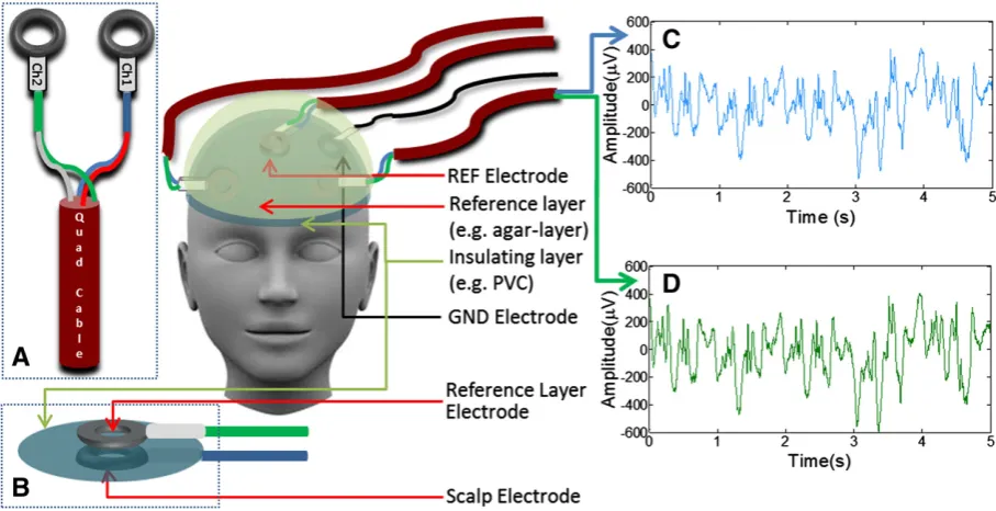
[image:3.595.75.529.487.720.2]

In the reference layer set-up, the paths of the leads connected to the electrodes on the scalp or phantom surface should match precisely with those of the leads connected to the corresponding electrodes on the reference layer all the way from the electrodes to

(4)

the EEG ampliﬁer. This ensures that artefact voltages induced in the two associated leads by movement or temporally varying mag-netic_ﬁelds are identical. Here, to provide the best possible matching of wire paths, balanced pairs of wires in star-quad cable (LSZH Starquad Installation, Van Damme Cable, www.van-damme.com) were employed for each scalp-reference lead pair. The star-quad cable comprises four cores, which are wired as two pairs with oppos-ing conductors in the star connected at each end and which are tight-ly twisted with a short lay length, thus providing greattight-ly improved rejection of low frequency electromagnetic interference compared to standard two-core twisted cables. Each electrode pair was formed from two sintered Ag/AgCl (EasyCap, Herrsching, Germany) ring-electrodes which were connected to the wire pairs in the star-quad cable using short (less than 7 cm) sections of standard single core wire (Fig. 1A). One electrode from each pair was attached to the scalp/phantom surface using abrasive and conductive gel (Abralyte 2000 EEG gel) and each reference layer electrode was positioned atop the corresponding scalp/phantom electrode (Fig. 1B) with the short sections of standard wire from the two electrodes laid atop one another. A thin insulating layer of polyvinyl chloride was used to separate the electrodes on the scalp/phantom from those on the reference layer (Fig. 1B). The reference layer was then placed over the electrode assembly and conductive gel was used to create good connections between the reference layer electrodes and the refer-ence layer. The ground (GND) electrode was attached to the scalp/ phantom, but also shorted to the reference layer by using conductive gel to form a bridge between the scalp/phantom and the reference layer through a small hole in the insulating layer, thus providing a common ground in the two layers. The approximately 5-mm-thick reference layer was constructed from saline-doped agar, which was produced using the same recipe as employed for manufacturing the

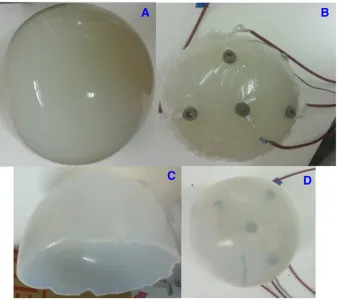
spherical phantom. Hemispherical or head-shaped layers (for use with the spherical phantom or human subjects respectively) were produced by using appropriately shaped_ﬁbre-glass moulds. Five electrode pairs were employed in this work. One pair formed the reference electrode pair (where the electrode used as the ampliﬁer's reference input was attached to the scalp) which was placed central-ly on the scalp. The remaining electrode pairs were positioned approx-imately equidistant from the reference electrode pair. The star-quad leads connected to each electrode pair were routed under the gel layer before exiting at the left or right side of the head/phantom, coming together under the chin to form a cable bundle, which then curved be-hind the receiver RF coil to run axially along the bore to the rear of the magnet. Leads attached to electrodes positioned on the right (left) side of the head/phantom exited from under the reference layer on the right (left) side of the head/phantom. The lead attached to the centrally posi-tioned reference electrode pair exited on the right hand side of the head/phantom.Fig. 2illustrates the steps followed in assembling the prototype reference layer set-up when carrying out experiments on the spherical phantom.

[image:4.595.126.464.412.712.2]

1-m long star-quad cables were run axially along the magnet bore and used to connect the electrodes to the EEG amplifier via a break-out box. We took a number of steps to isolate the cables, break-break-out box and EEG amplifier from vibrations produced by the scanner dur-ing imagdur-ing in order to limit the generation of additional artefacts as a result of movement of these components in the strong magnetic field. Specifically, the break-out box and EEG amplifier were placed on a table positioned just outside the bore of the magnet and the star-quad cables were tied together and attached to a cantilevered beam which wasfixed to the table (Mullinger et al., 2013a). The cable paths were kept as similar as possible for all recordings so as to limit variation of any voltages induced in the cables.

(5)

Data acquisition

Experiments were carried out in a Philips Achieva 3 T MR Scanner (Philips Medical Systems, Best, Netherlands) using a whole-body radiofrequency (RF) transmit coil and an eight-channel, head receive coil. A standard, axial multi-slice EPI sequence was implemented with TR = 2 s, TE = 35 ms, SENSE factor 2, a 36 × 36 matrix, 7 mm isotropic resolution and afive slice volume. A relatively coarse resolution was used so as to limit the maximum rate of change of the applied gradients, thus ensuring that the GA induced on the scalp or reference leads never exceeded the amplifier's dynamic range. This is not a pre-requisite of the RLAS approach, but was im-portant here as we wanted to compare directly the voltages induced in the scalp and reference layer leads. As the cap was constructed without series resistors, the imaging sequence for studying human subjects was designed without RF. Seventy volumes were acquired and thefive slice acquisitions were equally spaced within each TR-period. The TR and number of slices were chosen to ensure that the duration of each slice acquisition was an integer number of EEG-clock periods (the clock period was 200μs) as is required to allow optimal GA correction using AAS (Mandelkow et al., 2006; Mullinger et al., 2008c).

EEG data were recorded using a BrainAmp MR plus EEG ampliﬁ -er and Brain Vision Record-er software (Brain Products, Gilching, Germany). The EEG system allowed recording of signals in the frequency range 0.016–250 Hz with a sampling rate of 5 kHz. The MR scanning and EEG sampling were synchronised by driving the EEG ampliﬁer clock using a 5 kHz signal derived from a 10 MHz reference signal from the MR scanner (Mandelkow et al., 2006; Mullinger et al., 2008c). A TTL pulse generated by the scanner at the start of each slice acquisition was recorded by the EEG software. The pulse timing information was used to facilitate GA correction using AAS and to inform the analysis of average residual artefacts after application of the various correction methods.

A pair of electrodes attached to the chest (one at the mid-line and the other to the left of the heart) was used in conjunction with a BrainAmp ExG MR bipolar ampliﬁer and Brain Vision Recorder soft-ware (Brain Products, Munich, Germany) to record the subject's ECG during EEG recording. The ECG trace was used for the R-peak detec-tion that is required for PA correcdetec-tion when using the AAS technique.

Experiment 1: phantom

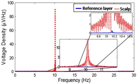
Aﬁrst experiment was carried out on the spherical phantom outside the scanner to test whether the use of RLAS with the proto-type reference layer set-up compromised the detection of neuronal signals. A primary assumption of the RLAS method is that the electri-cal isolation between the two layers ensures that signals generated in the brain (or phantom) are not detected at the reference layer electrodes and so are not affected when the difference of the scalp and reference layer signals is calculated. To test if any activity coming from the phantom was also detected by the reference layer, a 1 cm long current dipole was embedded in a spherical agar phan-tom with the dipole positioned close to the surface of the sphere. Signals from the scalp and reference layer electrodes were recorded from the phantom while a 10.2 Hz sinusoidal oscillating current was applied to the dipole so as to simulate a neuronal signal from the brain corresponding to peak–peak (p–p) dipole strength 20 ± 2 nAm.

Experiment 2: phantom

This experiment, which was carried out with the phantom in the scanner, was designed to compare the efﬁcacy of GA and MA correction using RLAS alone, RLAS followed by AAS (RLAS–AAS) and AAS only. In addition we tested the effectiveness of using RLAS and RLAS–AAS in comparison to the use of AAS alone in recovering a sinusoidal signal produced by a current dipole embedded in the phantom from EEG

data affected by both GA and MA. For this purpose, EEG data were recorded from the phantom in four different situations.

Experiment 2a—GA only.EEG data were recorded from the stationary phantom during execution of the multi-slice EPI sequence.

Experiment 2b—MA only.To simulate the effects of the head movements that occur during fMRI, data were recorded while the phantom was moved, in a continuous, periodic manner, inside the magnet bore continuously for approximately 30 s without the application of MR gradients. The amplitude of movements was limited so that the maxi-mum displacement of points of the sphere's surface was around 7 mm or less. In these and other phantom experiments involving MA, move-ments were generated by one of the investigators, who lightly pushed and then released the phantom, so as to cause small rotations and translations.

Experiment 2c—GA and MA.In this case, data were recorded while the phantom underwent controlled movements during execution of the EPI sequence. The phantom was moved up to three times dur-ing the whole acquisition with the number and size of the rotational and translational movements varied across the four datasets which were acquired (1 small movement ofb0.2 mm magnitude, 3 small movements ofb0.5 mm, 1 large movement ofb5 mm and 3 large movements ofb7 mm over the whole acquisition). The duration of each period of movement was approximately 4 s.

Experiment 2d—GA and MA with sinusoidal current present.The record-ings described under Experiment 2c were repeated (1 small move-ment ofb0.2 mm magnitude, 1 large movement ofb1 mm, 3 small movements ofb0.5 mm and 3 large movements ofb3 mm over the whole acquisition) using the phantom containing a current dipole, while the dipole was driven with a sinusoidal current at a frequency of 11 Hz (as described in Experiment 1) so as to mimic neuronal activity.

Experiment 3: human subjects

The_ﬁnal set of experiments was designed to assess the effectiveness of RLAS and RLAS–AAS compared with AAS when applied to data recorded from human subjects in the presence of GA, MA and PA. Two of the electrodes were placed over the visual cortex (to measure alpha power) and the other two either placed over the temples (to maximise sensitivity to the PA) or over the frontal lobe. To ensure subject safety, the RF pulse amplitude was set to zero as the cap conﬁguration had not fully been tested for RF heating effects and there were no series resistors between the electrodes and leads in this prototype cap. All EEG measurements described below were made on two healthy volunteers in four different situations.

Experiment 3a—PA.Recordings were made from two subjects inside the MR scanner with no MR gradients applied. The subjects were asked to remain still so that the PA was the dominant artefact.

Experiment 3b_—MA only.To simulate the effects of the head move-ments that occur during fMRI due to small movemove-ments, data were recorded while the subject moved (gentle nodding or shaking of the head, causing head movement of less than 5 mm in magnitude) inside the magnetic bore continuously for approximately 30 s with-out the application of MR gradients. This experiment was carried with-out on both subjects.

(6)

Experiment 3d—GA, PA and MA.Two recordings were made from the subjects during execution of the multi-slice EPI sequence. During the ﬁrst recording, the subject was asked to make one head movement (gentle head nod) during the acquisition, while in the second recording, three movements (gentle head nods) were made during the acquisition. The approximate duration of each period of movement was 5 s.

Experiment 3e—GA, PA and MA with changes in neuronal activity.It is well known that alpha activity (8–13 Hz neuronal oscillations) measured with EEG is strong in healthy individuals at rest with their eyes closed, and is suppressed by opening the eyes (Adrian and Matthews, 1934). Therefore to test the effect of RLAS on the detection of neuronal activity, an experiment was carried out in which changes in alpha activity were induced by asking the subjects to open their eyes for 30 s and then to close them for 30 s. During this period, EEG recordings were made while the multi-slice EPI se-quence was executed. The subject was also asked to move their feet (to cause small head rotations and translations typical of longer fMRI experiments) (Mullinger et al., 2011) for a_ﬁve second period during the recording.

Analysis

Initial analysis steps for RLAS and AAS were carried out using Brain Vision Analyzer 2 (Version 2.0.1; Brain Products, Munich, Germany) while MATLAB (The MathWorks) was used for further quantiﬁcation of the efﬁcacy of artefact correction that could be achieved using the different methods.

Artefact removal using RLAS

To implement RLAS, the reference layer signals were re-referenced using Brain Vision Analyzer 2 to the channel in the reference layer which overlaid the electrode on the scalp/phantom that was connected to the ampliﬁer's reference input. Raw EEG signals were high-pass ﬁltered with a 0.02 Hz cut-off frequency to remove any slow drifts. The signal from each reference layer electrode was then subtracted from the corresponding scalp electrode signal to yield RLAS-corrected EEG signals.

Artefact correction using AAS

The GA correction process used an average artefact waveform of 400 ms duration, formed from the average over all of the slice periods that were identi_ﬁed using the scanner-generated markers. This average slice artefact template was then subtracted from each occurrence of the GA. AAS was carried out on the raw scalp recordings (AASGA) and RLAS

corrected data (RLAS–AASGA). No additionalﬁltering or down-sampling

was applied during the artefact removal process.

PA correction was carried out on the data that had been acquired on the human subjects after gradient artefact correction. Here, the AAS method (Allen et al., 1998) used templates of the PA formed from the preceding 10 s of data recorded on each channel. These were formed by using R-peak markers derived from the ECG trace in conjunction with the direct detection method (Allen et al., 1998) in the Brain Vision Analyzer software. Any incorrectly positioned R-peak markers were manually repositioned. The EEG recordings were then segmented using the R-peak markers (−100 ms to + 600 ms in extent relative to R-peak) and baseline-corrected based on the 100 ms of data recorded before each R-peak (−100 ms to 0). The template on each channel was then subtracted from the data to eliminate each occurrence of the PA. PA correction via AAS was carried out on the AASGAdata (AASGA–AASPA) and the RLAS–AASGA

data (RLAS–AASGA–AASPA) to enable assessment of the total possible

gain in performance of artefact corrections which can be achieved by using RLAS in conjunction with post processing methods.

Evaluation of correction methods

To evaluate the ef_ﬁcacy of GA correction, the corrected data from Experiments 2 and 3 were exported to MATLAB, where the RMS magnitude of the artefact voltages over time was calculated from the raw data and then from data that had been subjected to: (i) AASGA, (ii) RLAS and (iii) RLAS–AASGA. Results were converted

to attenuation relative to the raw signal for each channel for each data set and the mean, maximum and minimum attenuation over channels was evaluated.

The effectiveness of PA correction was assessed by calculating the average and standard deviation of the pulse artefact waveform (from data acquired in Experiment 3a), before and after PA correction using AASPA, RLAS and RLAS–AASPA. In addition the reduction in the RMS of

the artefact voltages due to application of AASGA–AASPA, RLAS and

RLAS_–AASGA–AASPAwas calculated from the data acquired in

Experi-ment 3c to allow evaluation of the efﬁcacy artefact correction in the presence of pulse and gradient artefacts.

Motion artefacts cannot be corrected using AAS, so our analysis of MA correction focused on testing the efﬁcacy of RLAS. This was done by calculating the RMS amplitude of the signal during periods of movement before and after application of RLAS.

To test the capability of RLAS to remove the artefacts without af-fecting signals of interest, power spectra were calculated from the data acquired in Experiments 2d and 3e before and after correction using the different approaches.

Results

Verifying theﬁdelity of the RLAS approach

Fig. 3shows spectra of the signals sampled from electrodes on the spherical phantom and reference layer in Experiment 1. A strong peak resulting from the 10.2 Hz current that was applied to the dipole embedded in the agar sphere is evident in the spectrum from the

“scalp”electrode, but is almost absent (91 dB attenuation compared with the scalp signal) in the spectrum of the signal from the reference layer electrode.

[image:6.595.312.542.571.712.2]

Figs. 1C & D show example traces recorded from a reference layer electrode and associated scalp electrode on the phantom while the phan-tom underwent small continuous movements inside the scanner in Experiment 2b. The strong similarity of the artefact voltages in the two traces, which forms the basis of RLAS, is evident.Fig. 4shows that the artefact voltages appearing in the reference and scalp traces are similar during multi-slice EPI acquisition for the phantom (Experiment 2) and

(7)

human subject (Experiment 3c), and also show a high degree of similarity during the head movements that were made in the absence of time-varying MR gradients in Experiment 3b.

Comparing artefact removal methods

Phantom data

Fig. 5 shows a portion of the EEG trace recorded from a scalp electrode on the stationary phantom during the multi-slice EPI ac-quisition of Experiment 2a. Corresponding traces produced after correction using AASGA, RLAS and RLAS–AASGAare also shown. The

strong gradient artefacts repeatedﬁve times in each 2 s TR period can be seen clearly in the raw trace (blue) and in a greatly attenuated form in the trace produced after RLAS (green). With the phantom stationary, the GA is highly reproducible across repeated slice acquisitions and AAS (pink) consequently performs very well pro-ducing a reduction of the RMS voltage averaged across lead pairs of 26 dB (maximum/minimum = 31/21 dB) compared to the raw data, while RLAS yields a 24 dB attenuation (maximum/minimum = 29/17 dB). Further attenuation of the artefacts was achieved by performing RLAS followed by AASGA(red trace), yielding an average

41 dB reduction (maximum/minimum = 44/38 dB) of the RMS voltage relative to the raw data and leaving the cleanest signal with a maximum (p–p) signal range of 20μV (See also Supplementary Table S1).

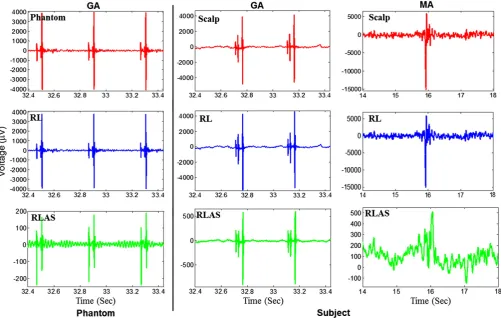
Fig. 6shows the effect of RLAS on the MA produced when the phantom was moved inside the scanner (in the absence of scanning) in Experiment 2b. Movement-induced voltages of more than 10 mV in amplitude are evident in the raw data (blue trace), but are greatly attenuated by the application of RLAS. In these data, the RMS artefact voltage over the whole acquisition was attenuated by 30 dB (maximum/minimum = 35/25 dB) by RLAS.

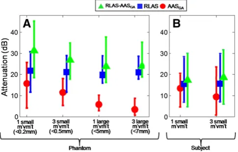
[image:7.595.52.554.53.371.2]

Fig. 7A characterises the efﬁcacy of artefact correction that was pro-duced by applying the different correction methods to data recorded

[image:7.595.46.292.490.702.2]

Fig. 4.Left column: EEG signal recorded from an electrode on the spherical phantom during the execution of the multi-slice EPI sequence (blue); re-referenced signal from the correspond-ing reference layer electrode (red); the difference of phantom and RL produced by RLAS (green). Middle Column similarly colour-coded signals recorded from a human subject durcorrespond-ing execution of the multi-slice EPI sequence. Right most column: similar signals recorded from human subject undergoing head movements in the 3 T static magneticﬁeld. Note that different voltage ranges have been used for these plots, since the RLAS data spans a much smaller voltage range than the recordings from the scalp of reference layer.

Fig. 5.Raw EEG signals recorded over 3 s from the stationary phantom during execution of multi-slice EPI sequence (blue) and after correction using AASGA(purple), RLAS (green)

and RLAS–AASGA(red). Inset shows expanded plots of AASGA, RLAS and RLAS–AASGA

(8)

from the phantom in Experiment 2c, in which the phantom underwent different degrees of movement during a multi-slice EPI acquisition. The markers indicate the average over channels of the attenuation of the RMS voltage, while the tips of the error bars indicate the maximum and minimum attenuation across channels. Thisﬁgure indicates that RLAS outperforms AASGAin all experiments and that implementing

AASGA after RLAS provides further attenuation of artefacts. The

performance of AASGAis particularly compromised when multiple,

large movements occur.

Fig. 8shows data that were recorded from one electrode pair at-tached to the phantom containing the current dipole in Experiment 2d, during which the phantom was moved while the multi-slice EPI acquisition was executed. Raw data (blue trace) from a 1.2 s period of the recording (within the 4 s movement epoch) are shown inFig. 8A, along with corresponding traces produced after correction using AASGA

(purple), RLAS (green) or RLAS–AASGA(red). The GAs occurring every

0.4 s are strongly evident in the raw data (the 988μV peak-to-peak am-plitude of the GA exceeds the ±400μV range shown in the plot). Residual GAs appear with much reduced amplitude in the RLAS data, but are removed by the subsequent application of AAS. There are signiﬁcant residual motion artefacts in the AASGAdata which mask the 11 Hz

signal from the current dipole, but this signal is evident in the RLAS data even before application of AAS. For the phantom data of Exper-iment 2d, the RMS artefact voltages averaged over all channels were attenuated on average by 19 dB (maximum/minimum = 23/15 dB), 20 dB (maximum/minimum = 26/12 dB) and 25 dB (maximum/ minimum = 29/19 dB) by using AASGA, RLAS and RLAS–AASGA

re-spectively (See also Supplementary Table S1).Fig. 8B shows the

power spectra calculated from the data recorded over the whole 140 s of the experiment.

Human subject data

Fig. 4clearly shows the similarity of the GA and MA in the traces from the reference layer and scalp leads in data from Subject 1. This indicates that the voltages generated by temporally varying magnetic ﬁeld gradients are similar on the reference layer and scalp leads, despite the non-spherical shape of the head and reference layer, and that this is also the case for voltages due to rotation in a uniform magneticﬁeld.

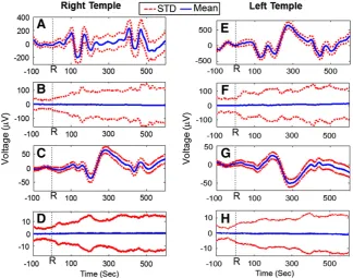
Fig. 9shows data from Experiment 3a in which recordings were made while Subject 1 lay stationary in the scanner with no scanning occurring, so that the PA was the dominant artefact. Raw data from elec-trodes attached to the right and left temples are shown, along with data corrected using AASPA, RLAS and RLAS–AASPA. Figs. 9A/E show the

average PA waveform recorded from the scalp electrode positioned on the right/left temple over 150 cardiac cycles occurring in a 2-min period. The standard deviation of the voltage across the 150 cardiac cycles is also indicated at each time point using dotted lines.Figs. 9B/F show the average and standard deviation of the PA after application of AASPA

to raw data from the right/left temple, whileFigs. 9C/G show data after application of RLAS andFigs. 9D/H show data resulting from the ap-plication of RLAS and AASPA. As expected, AAS reduces the average PA

approximately to zero, but there is a signiﬁcant variation of the re-sidual PA across cardiac cycles, which is indicated by the standard deviation of around 100μV shown inFigs. 9B & F. After application of RLAS the amplitude of the average PA is signiﬁcantly attenuated (right/left peak-to-peak voltage in raw data 402/1013μV versus 85/76μV in RLAS data) and the standard deviation of the PA is also reduced (Figs. 9C & G). The reduced variability of the PA is particular-ly evident in the RLAS–AASPAdata produced by applying both RLAS

[image:8.595.132.458.52.184.2]

and AAS to the data. Comparing the plots shown inFigs. 9D/H to those in B/F indicates that the standard deviation across cardiac cy-cles is reduced by a factor of around 10 by use of RLAS.

Fig. 10shows EEG data recorded from an electrode pair located on the right temple in Experiment 3c in which Subject 1 remained still during execution of the multi-slice EPI sequence, yielding maximally reproducible GA and PA. Raw data (blue) recorded over a 2 s period is shown inFig. 10A along with data corrected using the following combi-nations of correction methods: AASGA(purple), AASGA–AASPA (light

green), RLAS (dark green), RLAS–AASGA(red) and RLAS–AASGA–AASPA

(blue). The corrected data are shown on an expanded scale inFig. 10B. GA with peak-to-peak amplitude of more than 4 mV is evident in the raw data (Fig. 10A) and also appears with much reduced amplitude in the RLAS data (Figs. 10A & B). After GA correction using AAS, a PA of around 400μV peak-to-peak amplitude is evident in the AASGAdata

and is also seen, but with a signiﬁcantly reduced amplitude in the RLAS–AASGAdata. The latencies of the peaks of the PA relative to the

occurrence of the R-peak, which can be gauged by comparison to

Fig. 6.Raw EEG data recorded from the spherical phantom over an 8 s period of movement in the static magneticﬁeld (blue) and after RLAS (red).

Fig. 7.Mean RMS attenuation over channels for the phantom (A) and subject (B) data after correction with AASGA(red), RLAS (blue) and RLAS–AASGA(green) for varying degrees of

[image:8.595.39.282.548.703.2]

(9)

the ECG trace shown inFig. 10C, are similar to those shown inFig. 9. The PA is signiﬁcantly attenuated by application of AAS yielding the AASGA–AASPA and RLAS–AASGA–AASPA data. Comparison of these

two traces indicates that the noise level in the data that have been subjected to RLAS is signiﬁcantly reduced, presumably due to a re-duction of residual GA and PA, as well as MA due to small subject movements. Analysing the data from all leads over the whole re-cording we found that the RMS voltages were attenuated relative to the raw data by 11 dB (maximum/minimum = 14/5 dB), 14 dB (max./min. = 17/8 dB), 15 dB (max./min. = 16/14 dB), 25 dB (max./min. = 28/20 dB) and 27 dB (max./min. = 29/24 dB) by AASGA, AASGA–AASPA, RLAS, RLAS–AASGAand RLAS–AASGA–AASPA,

respectively (See also Supplementary Table S2).

The aspects of thesefindings related to the GA are confirmed by the plots shown inFig. 7B, which depict the efficacy of GA correction that was produced by applying the different correction methods to

data recorded in Experiment 3d, in which the two subjects executed different degrees of movement during a multi-slice EPI acquisition. As was found in the case of the moving phantom (Fig. 7A) RLAS out-performs AASGAin all experiments and implementing AASGAafter

RLAS provides further attenuation of artefacts.

[image:9.595.99.509.55.180.2]

Fig. 11shows the results from Experiment 3e in which changes in alpha activity between eyes-open and eyes-closed conditions were measured during scanning, with Subject 2 executing foot movements over a 5 s period during the one minute experiment.Fig. 11A shows power spectra from the 30 s-epoch during which the subject's eyes were open. These were produced using RLAS and are shown before (red) and after (blue) application of AAS for correction of the GA. Spec-tra produced from scalp data after application of AAS for GA and PA correction (green) are also shown. Data were taken from an electrode pair located over the occipital lobe, while the reference channel was positioned close to the Cz position in the 10/20 system.Fig. 11B shows

Fig. 8.EEG signals recorded from the spherical phantom containing a current dipole, which was driven with a current varying at 10.2 Hz, during execution of the multi-slice EPI sequence and movement of the phantom. Raw data (light blue) and data formed after correction using AASGA(purple), RLAS (green) and RLAS–AASGA(red) are shown over a 1.2 s period (A) along

[image:9.595.140.465.455.710.2]

with the square root of the power spectra (B).

Fig. 9.A representative single subject EEG trace from a right/left temple channel averaged over all cardiac cycles occurring in a 2-min period before (A/E) and after correction using AASPA

(B/G), RLAS (C/F) and RLAS–AASPA(D/H), with the dashed lines indicating the standard deviation of each average waveform. In these traces, R corresponds to the occurrence of the R-peak

(10)

similar data for the 30 s eyes-closed period. Inspection of the expanded plots spanning the 8–12 Hz frequency range shows similarly increased power in the alpha frequency range in the eyes-closed condition in all data, indicating that application of RLAS has not signiﬁcantly affected the measurement of brain signals. In particular, the increase in alpha power is clear in the RLAS data (red) which has not been subject to any additional post-processing.

Discussion

The results of the experiments carried out using the prototype reference layer system indicate that RLAS forms a viable method for attenuating at source the artefacts that are generated in EEG data recorded during concurrent fMRI experiments by time-varying magneticﬁeld gradients, cardiac pulsation and head movements. The results also demonstrate that RLAS can be used in conjunction

with AAS further to attenuate gradient and pulse artefacts and that the use of RLAS does not confound the recording of brain signals.

The results of Experiment 1 (Fig. 3) demonstrate that in the model system consisting of a current dipole embedded in a conducting agar sphere, voltages resulting from a time-varying current in the dipole are not sensed by reference layer electrodes, although they are picked up by electrodes on the phantom's surface. Consequently RLAS does not attenuate the voltage produced by the current dipole inside the sphere and can be expected similarly to preserve brain signals generat-ed at the scalp surface in human studies. This is borne out by the results of Experiment 3e (Fig. 11) in which an elevation in the alpha power as a result of the subject closing their eyes is still clearly detected when RLAS is applied.

The results of Experiment 2 demonstrate the efficacy of RLAS in attenuating the GA and MA under ideal conditions, in which: (i) the ref-erence layer forms a hemisphere which accurately overlays a spherical conductor; (ii) there are no brain signals nor PA to add to the signal variance; and (iii) movements are under the control of the experiment-er. The similarity of the artefact voltage waveforms recorded from the scalp and reference layer electrodes when the phantom is moved in the 3 T magneticfield or the time-varying gradients needed for imple-mentation of multi-slice EPI are applied is evident from the plots shown inFigs. 1 and 4, respectively. This similarity underlies the large reduction in the artefact voltages which are produced when RLAS is applied (Figs. 4–6).Fig. 6shows clearly that MA produced by random movements, which cannot be corrected using post-processing methods, is greatly reduced (30 dB attenuation) by RLAS, whileFigs. 4 and 5show that RLAS also greatly attenuates the GA. The residual GA in the RLAS data shown inFigs. 4 and 5indicates that the cancellation is not perfect, but it is evident from thesefigures that the peak artefact is reduced by more than an order of magnitude by application of RLAS. Quantitative analysis of the data from Experiment 2a shows that AASGAslightly

outperforms RLAS in attenuating the GA produced when the phantom is stationary (26 dB vs 24 dB). The conditions of Experiment 2a form an ideal basis for the implementation of AASGA, since the GA is expected

to be highly reproducible across repeated acquisitions in a stationary phantom. However the largest attenuation of the GA (41 dB) was pro-duced when AASGAwas applied in conjunction with RLAS, indicating

that the residual artefacts remaining after RLAS are stable across repeat-ed image acquisitions. These artefacts most likely result from small differences in the voltages induced in the reference layer compared with those appearing at the surface of the spherical phantom and also from the effect of small differences in the paths followed by the leads joining the two electrodes to the star-quad cable. The greater reduction in GA produced by using RLAS and AASGAtogether compared with the

use of AASGA alone implies that there are some GA contributions

[image:10.595.38.276.52.292.2]

which vary across repeated acquisitions, but which are similar in the reference layer and scalp channels. Such artefacts could arise from

Fig. 10.(A) EEG signal recorded from an electrode on the left temple over a 2 s period during execution of the multi-slice EPI sequence (blue) and (B) after correction using AASGA(purple), AASGA–AASPA(light green), RLAS (dark green), RLAS–AASGA(red) and

RLAS–AASGA–AASPA(blue). (C) Corresponding ECG trace with R peaks, marking the

onset of each cardiac cycle, depicted. Note that different voltage ranges have been used in each sub-plot so as to display clearly the detail of the signal waveforms.

[image:10.595.87.503.583.720.2]

(11)

small movements of the phantom in the static ﬁeld resulting from gradient coil vibrations.

When the phantom was moved during multi-slice EPI acquisition (Experiment 2c) the performance of AASGAwas compromised, with

the artefact attenuation reducing from 16 dB for the case where one small movement was made during the course of the 140 s recording to a value of 3 dB when three large movements occurred (Fig. 7). This failure of AASGAresults from changes in the GA waveform resulting

from changes in the position of leads and electrodes in the applied ﬁeld gradients, which mean that an average artefact template does not provide a good representation of individual artefact occurrences. In addition, the large, variable MA corrupts the average artefact template and leaves residual variance in the signal. In contrast, the performance of RLAS is relatively insensitive to the degree of movement, yielding a reduction of more than 20 dB over full range of movements that were employed (Fig. 7). The additional artefact attenuation produced by ap-plying AAS after RLAS is reduced as the degree of movement increases, presumably because the residual artefacts after application of RLAS are also sensitive to the positions of the lead and electrode pairs in the appliedﬁeld gradients. However even when the phantom was moved three times in the 140 s acquisition yielding electrode dis-placements of up to 7 mm, it was still possible to attenuate the artefacts by 25 dB using RLAS in combination with AASGA.

The results of Experiment 2d indicate that even in the presence of large GA and MA, RLAS is able to reveal the temporal evolution of an 11 Hz signal of ~50μV p–p amplitude from the embedded dipole (Fig. 8). While AASGAalso preserves the oscillatory 11 Hz signal it leaves

residual artefacts across a broad frequency spectrum, so that it is possi-ble to identify the signal from the dipole in the spectrum, but not in the time domain (Fig. 8). When making in vivo measurements of rhythmic neuronal activity, which typically span a broader frequency range and have a lower amplitude than the signal from the current dipole, the re-sidual artefacts after AAS are likely to dominate the time domain and may make it difﬁcult to identify the signal of interest in the frequency domain as well. This is demonstrated inFig. 11, where, while it is possi-ble to identify activity in the alpha band (enhanced by the subject closing their eyes) the amplitude of this activity suggests that if the fre-quency of interest was in the delta band (b4 Hz) then the residual MA and PA in data corrected using AAS only would most likely swamp the neuronal signals. It is important to reiterate that using standard methods of artefact correction it is generally not possible to recover brain signals from EEG data recorded during a period of signiﬁcant head motion. Here, however, we have demonstrated that with the application of RLAS–AASGAthe underlying signals can be recovered

(Fig. 8). In future EEG–fMRI studies this could have the beneﬁt of reducing the number and duration of epochs where brain signals are in-accessible and could also reduce the occurrence of movement-induced spurious correlations between EEG and BOLD signals that have previous-ly been reported (Jansen et al., 2012).

The measurements on human subjects show that RLAS also signiﬁ -cantly attenuates MA and GA in the more complex situation where the reference layer must replicate the artefact voltages induced in the heterogeneous volume conductor formed by the human head and where the reference layer no longer has a simple hemispherical shape.

Fig. 4shows that the artefacts recorded from scalp electrodes when time-varying gradients are applied, or head movements occur, are still very similar to those recorded from the corresponding reference layer electrodes. Taking the difference of these recordings in RLAS thus signiﬁcantly attenuates the MA and GA. Analysis of the data recorded from the stationary subjects (Experiment 3c) showed slightly different relative performances of the different artefact correction approaches compared with the data from the phantom: in the human subjects, the GA was better corrected by RLAS (15 dB attenuation) than AASGA

(11 dB attenuation), but RLAS–AASGA(25 dB attenuation) still provided

the best result. The better performance of RLAS compared with AASGAin

the human data most likely results from the effect of small involuntary

movements of the subject's head, including those due to pulsatile blood ﬂow (Mullinger et al., 2013b). These cause small MA that cannot be corrected by AAS and also produce slice-to-slice variation of the GA that confounds the operation of AASGA. The results of Experiment 3d

(Fig. 7) indicate that the performance of RLAS in reducing the signal variance in the presence of MA and GA is also better than that of AASGAin the presence of cued head movements, and in addition the

performance of AASGAdegrades as the degree of movement increases,

while the attenuation achieved by using RLAS or RLAS–AASGAis similar

for the cases where the subject makes 1 or 3 movements.Fig. 7also shows that in general the fractional reduction of the mean RMS voltage that was produced by using RLAS was less in the human data than recordings from the phantom. This is in part because of the presence of other sources of signal variance, including voltages from brain activ-ity, which also affect the fractional reduction produced using AAS, but may also re_ﬂect greater differences between the gradient and move-ment artefact voltages induced in the human head and head-shaped reference layer compared with those occurring in the model system formed by the hemispherical reference layer and homogenous spherical phantom.

The data shown inFig. 9indicates that RLAS can reduce the peak to peak amplitude of the PA by more than a factor of four and also reduces the standard deviation of the PA across cardiac cycles by about a factor of 10. Since it is the variability of the PA, which often causes problems with its correction in EEG–fMRI experiments, this finding promises significant benefit from use of RLAS in future studies. Overall, these measurements are consistent with the idea that the dominant source of the PA is cardiac-pulse-driven head movement (whose effect can be cancelled using RLAS) rather than Hall voltages due to bloodflow in the strong staticfield (which will not be affected by RLAS) (Mullinger et al., 2013b). In addition, the fact that the reduction of the standard de-viation of the PA across cardiac cycles due to RLAS is larger than the re-duction of the average magnitude of the PA implies that the artefact voltages due to cardiac-pulse-driven head movements contribute dis-proportionately to the variability of the PA. It is interesting to note that the temporal form of the PA shown in the raw data recordings in

Fig. 9is quite different from that previously reported (Debener et al., 2008) and its amplitude is also larger than in previously reported 3 T data. This difference in the temporal form of the PA compared with that found in recordings made using a conventional cap was seen on both subjects. It is most likely to be a consequence of the signiﬁcant differences between the lead paths used here and those which are employed in most EEG–fMRI experiments. The standard arrangement has the leads running over the surface of the head in a generally superi-or direction, starting from the electrodes and coming together in a cable bundle at the crown of the head, while in our experiments the leads ran in an inferior direction from the electrodes and left the scalp on the left or right side of the head depending on the location of the electrode. The voltages induced in the leads by head movements and pulse-driven scalp expansion and are likely to be quite different for these two arrangements and when combined withﬂow-induced Hall voltages could produce very dissimilar PA waveforms.

Fig. 10shows that applying AASPAto the RLAS–AASGAdata produces

(12)

layer is similar to that of brain tissue and so its addition does not produce any significant additional RF screening effects. The lead pairs and electrodes can also potentially be made of similar material to that used in current MR-compatible EEG systems and so would be expected to produce similar, minimal levels of RF and staticfield inhomogeneity. In the studies reported here, we used commercially available star-quad cable to form the lead pairs and since the configuration we employed had not been fully tested for RF heating effects (Mullinger et al., 2008b), the RF pulse amplitude was set to zero in the recordings made on the human subjects so as to avoid any risk of heating. Hence the impact of any MR artefacts due to RF is thus not being tested in the current study. A full evaluation of RF heating and effects on MR image quality will be car-ried out in the future as part of the development of an improved reference layer set-up. A small component of the GA is known to result from the RF pulses that are applied during MRI (Spencer et al., 2012). This contribu-tion to the GA would have been present in the data recorded from the phantom, but not in the data acquired from the human subjects, as the RF pulses were not applied in these experiments. Since the artefact reduc-tion produced by applying RLAS to the data from the phantom was excel-lent, we have no reason to believe that the performance of RLAS on data recorded from human subjects would be compromised by the presence of small RF pulse artefacts. However, further subject studies involving EPI acquisitions with the RF pulses enabled are needed to test this expectation.

The work described here has demonstrated the benefits in artefact reduction that RLAS can provide, but clearly for these benefits to be widely realised, it will be necessary to devise a more robust reference layer arrangement that is also easier to use. This will require the use of a reference layer material that is tougher than saline-doped agar, but which still has a similar conductivity to tissue. Carbon-fibre-loaded rubber and hydrogel form two candidate materials. In addition it will be helpful to establish how the geometry and shape of the reference layer affect the similarity of the artefact voltages induced in the refer-ence layer and scalp, so that an optimal referrefer-ence layer configuration can be designed. We are currently carrying out electromagnetic simula-tions to evaluate the effect on the induced gradient artefacts of changing the reference layer properties (Chowdhury et al., 2013).

For the work carried out here, we used unipolar EEG amplifiers with a common reference, so as to allow the artefact voltages from reference layer and scalp electrodes to be separately recorded and analysed. This meant that the maximum difference in voltage between the reference channel amplifier input and the inputs associated with all other elec-trodes had to be kept less than the amplifiers' dynamic range (32 mV). Consequently we used a multi-slice EPI sequence with a relatively coarse resolution when generating GA and also used a conservative, 250 Hz low-passfilter setting, to ensure that there was no clipping of signals. However, it is also possible to use the reference layer approach in conjunction with bipolar EEG amplifiers that are connected so as to measure the voltage differences between each reference layer and scalp electrode pair. Since the artefact voltages appearing on the inputs linked to the reference layer and scalp electrodes will be very similar for each pair, with this arrangement it would be possible to reduce the dynamic range required of the amplifiers compared with current MR-compatible EEG systems and also to open up the bandwidth of the system to allow recording of high frequency electric signals from the brain (Freyer et al., 2009) without causing saturation due to the increased peak amplitudes of the GA.

Conclusion

In conclusion we have shown that the RLAS technique is a viable method by which to remove artefacts in EEG data during simultaneous fMRI with no signal loss or distortion of the neuronal signals of interest. We have shown that RLAS generally outperforms AAS if any motion is present in the removal of the GA and PA and that using AAS in conjunction with RLAS produces the highest attenuation of the artefacts

present. In addition we have demonstrated the power of RLAS in removing MA, which generally cannot be corrected using post-processing methods, because their occurrence is unpredictable and they are highly variable in their temporal and spatial form.

Acknowledgment

This work was funded by EPSRC Grant EP/J006823/1 and a Com-monwealth Scholarship which was awarded to MEHC and an Anne McLaren Fellowship which was awarded to KJM.

Appendix A. Supplementary data

Supplementary data to this article can be found online athttp://dx. doi.org/10.1016/j.neuroimage.2013.08.039.

References

Adrian, E.D., Matthews, B.H.C., 1934.The Berger rhythm: potential changes from the occipital lobes in man. Brain 57, 355–385.

Allen, P.J., Poizzi, G., Krakow, K., Fish, D.R., Lemieux, L., 1998.Identiﬁcation of EEG events in the MR scanner: the problem of pulse artifact and a method for its subtraction. NeuroImage 8 (3), 229–239.

Allen, P.J., Josephs, O., Turner, R., 2000.A method for removing imaging artifact from continuous EEG recorded during functional MRI. NeuroImage 12 (2), 230–239. Amor, F., Rudrauf, D., Navarro, V., 2005.Imaging brain synchrony at high

spatio-temporal resolution: application to MEG during absence seizures. Signal Process. 85, 2101–2111.

Becker, R., Ritter, P., Moosmann, M., Villringer, A., 2005.Visual evoked potentials recovered from fMRI scan period. Hum. Brain Mapp. 26, 221–230.

Bencsik, M., Bowtell, R., Bowley, R.M., 2007.Electricﬁelds in the human body by time-varying magneticﬁeld gradients: numerical calculations and correlation analysis. Phys. Med. Biol. 52, 1–17.

Bonmassar, G., Purdon, P.L., Jaaskelainen, I.P., Chiappa, K., Solo, V., Brown, E.N., Belliveau, J.W., 2002.Motion and ballistocardiogram artifact removal for interleaved recording of EEG and EPs during MRI. NeuroImage 16 (4), 1127–1141.

Chowdhury, M.E.H., Mullinger, K.J., Bowtell, R.W., 2013.A novel method of minimizing EEG artefacts during simultaneous fMRI: a simulation study. 19th Annual Meeting of the Organization for Human Brain Mapping, Abstract#1783, Seattle.

Debener, S., Ullsperger, M., Siegel, M., Fiehler, K., Yves von Cramon, D., Engel, A.K., 2005. Trial-by-trial coupling of concurrent electroencephalogram and functional magnetic resonance imaging identiﬁes the dynamics of performance monitoring. J. Neurosci. 25 (50), 11730–11737.

Debener, S., Mullinger, K.J., Niazy, R.K., Bowtell, R.W., 2008.Properties of the ballistocardiogram artefact as revealed by EEG recordings at 1.5, 3 and 7 tesla static magneticﬁeld strength. Int. J. Psychophysiol. 67 (3), 189–199. Dunseath, W.J.R., Alden, T.A., 2009.Electrode Cap for Obtaining Electrophysiological

Mea-surement Signals from Head of Subject, has MeaMea-surement Signal Electrodes Extended through Electrically Conductive Layer and Insulating Layer for Contacting Head of Subject (USA, US 2009/0099473).

Freyer, F., Becker, R., Anami, K., Curio, G., Villringer, A., Ritter, P., 2009. Ultrahigh-frequency EEG during fMRI: pushing the limits of imaging-artifact correction. NeuroImage 48 (1), 94–108.

Goldman, R.I., Stern, J.M., Engel, J., Cohen, M.S., 2002.Simultaneous EEG and fMRI of the alpha rhythm. Neuroreport 13 (18), 2487–2492.

Gotman, J., Benar, C.G., Dubeau, F., 2004.Combining EEG and fMRI in epilepsy: meth-odological challenges and clinical results. J. Clin. Neurophysiol. 21 (4), 229–240. Hamandi, K., Salek-Haddadi, A., F., D.R., Lemieux, L., 2004.EEG/functional MRI in epilepsy:

the queen square experience. J. Clin. Neurophysiol. 21 (4), 241–248.

Ives, J.R., Warach, S., Schmitt, F., Edelman, R.R., Schomer, D.L., 1993.Monitoring a patient's EEG during echo planar MRI. Electroencephalogr. Clin. Neurophysiol. 87 (6), 417–420.

Jansen, M., White, T.P., Mullinger, K.J., Liddle, E.B., Gowland, P.A., Francis, S.T., Bowtell, R., Liddle, P.F., 2012.Motion-related artefacts in EEG predict neuronally plausible patterns of activation in fMRI data. NeuroImage 59 (1–3), 261–270. Laufs, H., Krakow, K., Sterzer, P., Eger, E., Beyerle, A., Salek-Haddadi, A.,

Kleinschmidt, A., 2003.Electroencephalographic signatures of attentional and cognitive default modes in spontaneous brain activityﬂuctuations at rest. Proc. Natl. Acad. Sci. U. S. A. 100 (19), 11053–11058.

Mandelkow, H., Halder, P., Boesiger, P., Brandeis, D., 2006.Synchronisation facilitates removal of MRI artefacts from concurrent EEG recordings and increases usable bandwidth. NeuroImage 32 (3), 1120–1126.

Mantini, D., Perrucci, M.G., Cugini, S., Ferretti, A., Romani, G.L., Del Gratta, C., 2007. Complete artifact removal for EEG recorded during continuous fMRI using inde-pendent component analysis. NeuroImage 34 (2), 598–607.

Masterton, J., Abbott, D.F., Fleming, S., Jackson, G.D., 2007.Measurement and reduction of motion and ballistocardiogram artefacts from simultaneous EEG and fMRI recordings. NeuroImage 37, 202–211.

(13)

Mullinger, K.J., Brookes, M.J., Geirsdottir, G.B., Bowtell, R., 2008a.Average gradient artefact subtraction: the effect on neuronal signals. Human Brain Mapping, Elsevier, Melbourne.

Mullinger, K.J., Debener, S., Coxon, R., Bowtell, R.W., 2008b.Effects of simultaneous EEG recording on MRI data quality at 1.5, 3 and 7 tesla. Int. J. Psychophysiol. 67, 178–188.

Mullinger, K.J., Morgan, P.S., Bowtell, R.W., 2008c. Improved artefact correction for combined electroencephalography/functional MRI by means of synchronization and use of VCG recordings. J. Magn. Reson. Imaging 27 (3), 607–616.

Mullinger, K.J., Yan, W.X., Bowtell, R.W., 2011.Reducing the gradient artefact in simultaneous EEG–fMRI by adjusting the subject's axial position. NeuroImage 54 (3), 1942–1950.

Mullinger, K.J., Castellone, P., Bowtell, R.W., 2013a.Best current practice for obtaining high quality EEG data during simultaneous fMRI. J. Vis. Exp. 76 (In press).

Mullinger, K.J., Havenhand, J., Bowtell, R.W., 2013b.Identifying the sources of the pulse artefact in EEG recordings made inside an MR scanner. NeuroImage 71, 75–83. Naizy, R.K., Bechmann, C.F., Iannetti, G.D., Brady, J.M., Smith, S.M., 2005.Removal of fMRI

environment artifacts from EEG data using optimal basis sets. NeuroImage 28 (3), 720–737.

Spencer, S.G., Mullinger, K.J., Peters, A., Bowtell, R.W., 2012.Modelling and removing the gradient artefact using a gradient modelﬁt (GMF). Proc. Intl. Soc. Mag. Reson. Med. 20, Abstract#2083. ISMRM, Melbourne.

Yacoub, E., Shmuel, A., Pfeuffer, J., 2001.Investigation of the initial dip in fMRI at 7 tesla. NMR Biomed. 14, 408–412.

Yan, W.X., Mullinger, K.J., Brookes, M.J., Bowtell, R.W., 2009.Understanding gradient artefacts in simultaneous EEG/fMRI. NeuroImage 46 (2), 459–471.