Loss cone evolution and particle escape in collapsing magnetic trap models in solar flares

DOI:10.1051/0004-6361/201322519 c

ESO 2014

Astrophysics

&

Loss cone evolution and particle escape in collapsing magnetic

trap models in solar flares

Solmaz Eradat Oskoui, Thomas Neukirch, and Keith James Grady

School of Mathematics and Statistics, University of St Andrews, St. Andrews KY16 9SS,UK e-mail:[se11;tn3]@st-andrews.ac.uk

Received 21 August 2013/Accepted 30 January 2014

ABSTRACT

Context.Collapsing magnetic traps (CMTs) have been suggested as one possible mechanism responsible for the acceleration of high-energy particles during solar flares. An important question regarding the CMT acceleration mechanism is which particle orbits escape and which are trapped during the time evolution of a CMT. While some models predict the escape of the majority of particle orbits, other more sophisticated CMT models show that, in particular, the highest-energy particles remain trapped at all times. The exact prediction is not straightforward because both the loss cone angle and the particle orbit pitch angle evolve in time in a CMT. Aims.Our aim is to gain a better understanding of the conditions leading to either particle orbit escape or trapping in CMTs. Methods. We present a detailed investigation of the time evolution of particle orbit pitch angles in the CMT model of Giuliani and collaborators and compare this with the time evolution of the loss cone angle. The non-relativistic guiding centre approximation is used to calculate the particle orbits. We also use simplified models to corroborate the findings of the particle orbit calculations. Results.We find that there is a critical initial pitch angle for each field line of a CMT that divides trapped and escaping particle orbits. This critical initial pitch angle is greater than the initial loss cone angle, but smaller than the asymptotic (final) loss cone angle for that field line. As the final loss cone angle in CMTs is larger than the initial loss cone angle, particle orbits with pitch angles that cross into the loss cone during their time evolution will escape whereas all other particle orbits are trapped. We find that in realistic CMT models, Fermi acceleration will only dominate in the initial phase of the CMT evolution and, in this case, can reduce the pitch angle, but that betatron acceleration will dominate for later stages of the CMT evolution leading to a systematic increase of the pitch angle. Whether a particle escapes or remains trapped depends critically on the relative importance of the two acceleration mechanisms, which cannot be decoupled in more sophisticated CMT models.

Key words.Sun: corona – Sun: activity – Sun: flares

1. Introduction

Collapsing magnetic traps (CMTs) have been suggested as one of the mechanisms that could contribute to particle energisation in solar flares (e.g.,Somov & Kosugi 1997). The basic idea be-hind CMTs is that charged particles will be trapped on the mag-netic field lines below the reconnection region of a flare. The magnetic field will evolve into a lower energy state, resulting in (a) a shortening of field line length and (b) an increase in the overall field strength. Due to the vast difference in length and timescales between the particle motion and the magnetic field evolution, the particle motion can be described to a large degree of accuracy by guiding centre theory. The conservation of a par-ticle’s magnetic moment and the bounce invariant (e.g.,Grady et al. 2012) give rise to the possibility of an increase in the par-ticle’s kinetic energy by betatron acceleration and by first order Fermi acceleration (e.g.,Somov & Kosugi 1997; Bogachev & Somov 2005).

Studies of CMTs using models with varying degree of detail, focusing on different aspects of CMT physics have be carried out (e.g.,Somov & Kosugi 1997). In this paper, we investigate one very important aspect of particle motion in CMTs, namely what determines whether particles remain trapped or escape during the evolution of a CMT. Answering this question is important to be able to assess whether the CMT mechanism can contribute to the energetic particle flux, causing hard X-ray emission from

the footpoints of flaring magnetic loops or whether it can be ex-pected to contribute more to emission originating from higher up in the corona (e.g.,Krucker et al. 2008).

At first sight, this may seem like a trivial question to answer because obviously as soon as a particle orbit moves into the loss cone it will escape from the CMT. However, on second thought, things are not as simple as they seem for two reasons: (a) the loss cone itself changes in time due to the changing magnetic field strength; and (b) the particle pitch angle also evolves due to betatron and Fermi acceleration. Generally, one would expect the magnetic field strength within a relaxing magnetic loop to increase. Assuming that the magnetic field strength is highest at the foot points and that this field strength does not change sub-stantially, the loss cone should generally open up during the evo-lution of a CMT. How much the loss cone opens depends on the magnetic field model (see, e.g.,Aschwanden 2004, for a model where the loss cone opens to 90◦). Furthermore, whereas in in-vestigations based on a number of simplifying assumptions (e.g., Somov & Bogachev 2003; Somov 2004;Bogachev & Somov 2005) some predictions can be made about, for example, the relative importance of betatron and Fermi acceleration and the resulting consequences. However, similar predictions are much harder to make for more detailed magnetic field models (e.g., Giuliani et al. 2005;Karlický & Bárta 2006;Minoshima et al. 2010;Grady et al. 2012) because the relative importance of beta-tron vs. Fermi acceleration: (i) will be different for particles with

different initial conditions; (ii) may change with time during the evolution of the CMT; and (iii) will depend on the details of the magnetic field model used. Furthermore, it is well known that in time-dependent and curved magnetic fields the two mechanisms are closely linked (see, e.g.,Northrop 1963).

The aim of this paper is to present a detailed investigation of particle escape and trapping for the CMT model ofGiuliani et al.(2005). For the purpose of this paper, we ignore pitch an-gle scattering by Coulomb collisions, wave-particle interaction, or turbulence. Pitch angle scattering will, of course, change the results, but we regard the present investigation as a benchmark with which possible future investigations, including the effects of pitch angle scattering, can be compared. In Sect.2, we give a brief outline of the CMT model ofGiuliani et al.(2005) and summarise some of the results ofGrady et al.(2012) that are rel-evant to this paper. In Sect.3, we investigate how the loss cone evolves in our CMT model and how the pitch angle of typical particle orbits change with time, and we try to give an expla-nation of our results on the basis of some simplified models in Sect.4. We present a summary of our results in Sect.5

2. Brief model overview

Giuliani et al.(2005) used the kinematic MHD equations,

E+u×B = 0, (1)

∂B

∂t = −∇ ×E, (2)

∇ ·B = 0, (3)

to develop a general framework for analytical CMT models, de-scribing the evolution of the magnetic field for a given flow velocity,u(x,t) under the assumption that the magnetic field is translationally invariant in the z-direction and the flow veloc-ity has vanishingvz(for an extension to fully three-dimensional

model, seeGrady & Neukirch 2009). It is assumed that thexand

zcoordinates run parallel to the solar surface andyrepresents the height above the solar surface.

Under the assumption of translational invariance, one can use a flux functionA(x, y) to write the magnetic field in the form

B=∇A×ez+Bzez, (4)

which automatically satisfies Eq. (3). The other two equations can be written as

dA

dt =

∂A

∂t +u.∇A = 0, (5)

∂Bz

∂t +∇.(Bzu) = 0, (6)

with the electric field given by E=−∂A

∂t· (7)

FollowingGiuliani et al.(2005) we will assume that Bz andvz

vanish.

A CMT model is then defined by choosing a form for the flux functionA0(x, y)=A(x, y,t0) at a fixed timet0, and by specify-ing a flow fieldu(x, y,t). In the theory ofGiuliani et al.(2005), instead of defining the flow field directly, it is given implicitly by choosing a time-dependent transformation between Lagrangian and Eulerian coordinates. The advantage is that one can then im-mediately solve Eq. (5) usingA0(x, y) as the initial or, as was the choice ofGiuliani et al.(2005), the final condition.

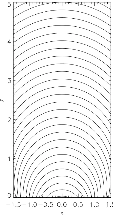
Fig. 1.Field line plot of the asymptotic state (t→ ∞) of the magnetic field of the CMT model used in this paper.

In this paper, we use the same magnetic field model as Giuliani et al.(2005) andGrady et al.(2012), which is given by

A0=c1

arctan

y0+d1

x0+w

−arctan

y0+d2

x0−w

· (8)

This flux function represents a potential magnetic field loop at timet0 (we assume that t0 → ∞) created by two line sources of strengthc1(one of positive and one of negative polarity) lo-cated at the positions (−w,−d1) and (w,−d2) below the lower boundary. All lengths here are scaled to a fundamental length scaleL. FollowingGiuliani et al.(2005), we choosew=0.5 and

d1=d2=1.0, creating a symmetric magnetic loop (Fig.1). The CMT model is completed by choosing the time-dependent transformation between Eulerian and Lagrangian co-ordinates. Again, we choose the same transformation as in Giuliani et al.(2005) andGrady et al.(2012), namely

x0 = x, (9)

y0 = (at)bln

1+ y (at)b

1+tanh(y−Lv/L)a1 2

+

1−tanh(y−Lv/L)a1

2 y. (10)

height the magnetic field is largely unchanged. The parame-tera1 determines the scale over which this transition from an unstretched to a stretched field takes place, whereasaandbare parameters that are related to the timescale of the evolution of the CMT. We use the same values for the parameters as in the previous papers, i.e.,a=0.4,b=1.0,Lv/L=1.0, anda1=0.9.

3. Evolution of pitch angle

θ

α

Due to the vast difference between the Larmor frequency and ra-dius of charged particle orbits and the time and length scales of the CMT model, one can safely make use of the guiding centre approximation for calculating particle orbits (see, e.g.,Giuliani et al. 2005). It turns out that theE×B-drift is by far the domi-nating drift and therefore the guiding centre remain on (or very close to) the same field for all times (see, e.g.,Grady 2012, for a detailed discussion).

We first briefly summarise the findings of Grady et al. (2012), who likeGiuliani et al.(2005) stopped the integration of particle orbits after a finite time (corresponding to 95 s in their normalisation). Grady et al.(2012) found that for most initial conditions the particle orbits remain trapped during this time. They also found that, not surprisingly, different initial po-sitions (x, y), initial energiesEand initial pitch anglesθhave an effect on the position of the mirror points, the energy gain of the particle orbits, and on whether they remain trapped or escape.

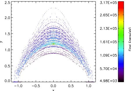
In particular, they found that the particle orbits that gain most energy during the trap collapse have initial pitch anglesθclose to 90◦and initial positions in a weak magnetic field region in the middle of the trap. These particle orbits with the largest energy gain remained trapped during the collapse and due to their pitch angle staying close to 90◦ have mirror points very close to the centre of the trap.Grady et al.(2012) argue that these particle orbits are energised mainly by the betatron mechanism. Other particle orbits with initial pitch angles closer to 0◦(or 180◦) seem to be energised by the Fermi mechanism at the beginning, but as already pointed out byGiuliani et al.(2005) and corroborated by Grady et al.(2012), these particle orbits gain energy when pass-ing through the centre of the trap. At later stages, these particle orbits also seem to be undergoing mainly betatron acceleration. We will make use of this result later in this paper. To illustrate these findings we show the positions and energies (colour-coded) at the end of the nominal collapse time of 95 s for a number of initial conditions in Fig.2. Particle orbits that have crossed the lower boundary (i.e., escaped) are represented by the dots on the

x-axis of the plot.

Before we start a more detailed investigation of particle trap-ping and escape in our CMT model, we recall a number of basic definitions that we make use of throughout the paper. We already mentioned the pitch angle of a particle orbit, which is defined as θ=arccos

_v v

, (11)

wherevis the velocity of the particle along the field line andv is the total velocity of the particle. We define the mirror ratio as

R(t)= Bfp

B(t), (12)

whereBfpis the foot point field strength of a particular field line andB(t) the field strength on the same field line atx = 0. The field strength at the foot points of the field lines basically re-mains constant over time because the transformation given in

Fig. 2.Graph of final position with corresponding energy. The colour bar gives the final energy of the trapped particles. The highest energies are found to be trapped in the middle of the trap.

Eqs (9) and (10) ensures that theBycomponent of the magnetic field on the lower boundaryy=0 does not change, although the

Bx component could change in time. This change is so small,

however, that one can regard the absolute value of the magnetic field strength at the footpoints as constant. The mirror ratioR(t) is related to the loss cone angle by

α(t)=arcsin

1 √

R(t)

· (13)

We emphasize that both the mirror ratio and the loss cone an-gle not only vary in time due to the time evolution of the mag-netic field, but also from field line to field line, but we have sup-pressed the spatial dependence in the definitions above for ease of notation.

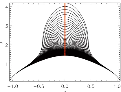
We start our investigation by looking in more detail at two particle orbits starting at the same initial position (x=0,y=4.2) and the same initial energy (5.5 keV), but with different initial pitch angles of 87.3◦(orbit 1) and 160.4◦(orbit 2). These initial conditions are representative of the typical behaviour of particle orbits with an initial pitch angle close to 90◦, which have very little movement along the field lines, and particle orbits which at the initial time have a much larger velocity component paral-lel (or in this case anti-paralparal-lel) to the magnetic field. The two sets of initial conditions chosen here are very similar (albeit not identical) to the two examples of orbits discussed inGrady et al. (2012), and thus the orbits (shown in Fig.3) are very similar to the orbits discussed in their paper. As one can clearly see in Fig.3, orbit 1 (red) remains confined to the middle of the trap due to the fact that the initial pitch angle is close to 90◦, whereas orbit 2 (black) has mirror points very close to the bottom bound-ary, but does not escape during the time of the calculation. We also point out that there is very little change in the position of the mirror points over time, which is consistent with previous findings (Grady et al. 2012).

Fig. 3.Two illustrative particle orbits starting at the same initial position

x=0,y=4.2 and with the same initial energy (5.5 keV), but different initial pitch angles. Orbit 1 (red) has an initial pitch angle of 87.3◦_(i.e.

close to 90◦) and hence stays close to the middle of the CMT at all times, whereas orbit 2 (black) has an initial pitch angle of 160.4◦_and

has mirror points close to the lower boundary.

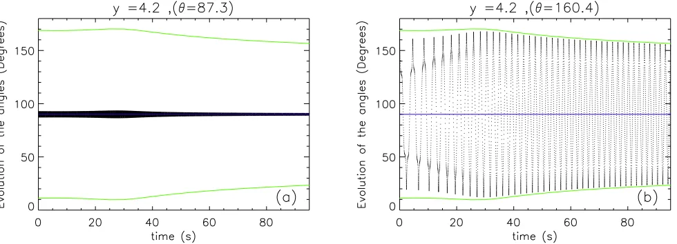
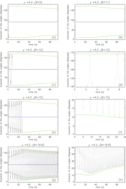
the top of the plots) because particle orbits will escape from the trap if their pitch angle becomes either less thanα(t) or larger than 180◦−α(t). Obviously, the graph of 180◦−α(t) here is just a mirror image of the graph ofα(t) when mirrored at the line 90◦ (shown in blue on the plots) because the CMT we consider here has a magnetic field that is symmetric with respect tox=0. The initial value of the loss cone angleα(t) for this particular mag-netic field line is 11.8◦and its value at the end of the calculation is 23.4◦. The asymptotic value of the loss cone angle in the limit

t→ ∞is, however, much larger, namely 44.8◦. As expected, the loss cone angle generally increases with time because the mag-netic field strength at the apex of the magmag-netic field line atx=0 increases with time. However, one can see from the plots that up to a time of roughly 30 s the loss cone angle is decreasing. This is a particular feature of the CMT model ofGiuliani et al.(2005), which in the initial stages of its time evolution has a region of very weak magnetic field through which the field lines have to move first, before the field strength starts to increase again. This is the reason for the initial dip in the graph of the loss cone angle. The asymptotic value of the loss cone angle does not approach 90◦ because we have an inhomogeneous asymptotic magnetic field with a larger field strength at the foot points compared to the highest points along field lines, and thus particle orbits can remain trapped in this CMT model (e.g., contrary to the model ofAschwanden 2004). We emphasize again that the values of the loss cone angle at all times are different for different initial positions, but that the qualitative behaviour is the same.

The time evolution of the pitch angle of particle orbits 1 and 2 is shown by the black dotted lines in Fig.4a and b, re-spectively. One can see in Fig.4a the pitch angle of particle or-bit 1 always remains very close to the blue 90◦angle. Although the oscillatory behaviour itself is very hard to see in the plot, the amplitude of the pitch angle oscillation is clearly decreasing as time progresses. This can be easily understood by recalling that Grady et al.(2012) showed that particle orbits of this type do not experience any significant changes in their parallel energy, whereas they gain considerable amounts of perpendicular energy due to betatron acceleration. From Eq. (11), it is clear that ifv remains roughly constant whilevincreases due to the increase in the perpendicular velocity thatθwill tend towards 90◦.

The more interesting of the two particle orbits shown is or-bit 2 (Fig.4b), because its pitch angle is much closer to the loss cone angle and thus close to escaping from the CMT. Before we start a detailed discussion of the features seen in the plot, we remark that the maxima and minima of the pitch angle curve correspond to the times when the particle orbit passes through the apex of the field line, whereas the mirror points correspond to the crossings of the 90◦line (blue). As already stated above, this particle orbit has an initial pitch angle of 160.4◦and there-fore a much larger initialvthan orbit 1. We see that in the first roughly 30 s the maximum (minimum) values of the pitch an-gle curve increasing (decreasing) are approaching the green loss cone angle curve. After this time the pitch angle maxima (min-ima) start decreasing (increasing) and follow the same trend as seen in the curves representing the loss cone angle and its mir-ror image, while still very slowly approaching those curves. This general trend seen in the pitch angle behaviour can be explained in a similar way to the behaviour of particle orbit 1 by the in-crease in magnetic field strength at the apex of the field line and the corresponding average gain in perpendicular energy due to betatron acceleration, with the main difference being that orbit 1 always remains close to the field line apex, whereas orbit 2 makes lengthy excursions down the field line almost to the lower boundary. The orbit does, however, not cross the lower boundary before the calculation was stopped.

We looked next at cases of particle orbits with the same ini-tial position and energy as orbits 1 and 2, but with iniini-tial pitch angles ofθ = 5◦, 11◦, 12◦, 15◦and 19.6◦. This covers a range of pitch angle values starting inside the initial loss cone angle of 11.8◦, just outside the initial loss cone angle and up to the initial pitch angle of 19.6◦, which is 180◦−160.4◦. The time evolution of the pitch angles for these orbits is shown in Fig.5, again with the curves for the loss cone angle (green) and the 90◦line (blue). The orbits with initial pitch angle values 5◦and 11◦(Fig.5a and b, respectively) escape from the CMT immediately without mirroring at all. This clearly is expected since their initial pitch angles are smaller than the initial loss cone angle. The orbits for initial pitch angles 12◦(Fig.5c), and 15◦(Fig5e) display a number of bounces within the CMT before escaping after they cross either the lower or the upper green curve representing the loss cone angle. Figure5c and e show the pitch angle evolution on the full scale, whereas Fig.5d and f show blow-ups of the relevant parts of the curves close to the loss cone angle curve. One can also see that the particle orbits display more bounces before escaping the CMT if their initial pitch angle is further away from the initial loss cone angle. For an initial pitch angle of 19.6◦in Fig.5g and its blow-up (h), we see the same behaviour as already described above. The minima and maxima of the pitch angle curve follow the same trend as the loss cone curve, but do not cross into the loss cone, albeit edging slightly closer to it as time progresses.

All particle orbit calculations discussed so far have been stopped at a time of 95 s well before coming close to the asymp-totic limit for the loss cone angles of 44.8◦. This raises the ques-tion of whether the orbits trapped att=95 s will remain trapped if the calculation is continued beyond this time. We have there-fore first increased the stopping time for the calculation of the particle orbit with an initial pitch angle of 160.4◦ (shown in Figs.3and4b) by a factor of approximately 100. The result of this calculation is shown in Fig.6a and it turns out that this par-ticle orbit eventually escapes from the CMT at a time of about 234 s (right-hand boundary of the plot).

Fig. 4.Evolution of the particle orbit pitch angleθ(black dotted line) compared with evolution of the loss cone angleα(green lines) for particle orbits 1 (left, initial pitch angleθ = 87.3◦) and 2 (right, initial pitch angleθ = 160.4◦). The blue line marks the 90◦point (see main text for discussion).

the long-term evolution of particle orbits by decreasing the val-ues of the initial pitch angle from 160.4◦to 155.4◦. The results are shown in the other plots in Fig.6b and c. We would like to point out that in each of the cases, the length of the time axis is set to either the time when the orbit escapes from the trap or to the time when the calculation is stopped (10 000 s). For initial pitch angle values smaller than 159.0◦(Fig.6b) we show only the maxima and minima of the pitch angle curve (the envelope of the curve created from the values of the pitch angle when the orbits is at the apex of the field line), because of the large num-ber of bounces the particle orbits undergo over the extended time period of the calculation.

As already stated above, the particle orbit with initial pitch angle of 160.4◦ escapes from the CMT at around t = 234 s. During further investigation a decrease in the value of the initial pitch angle by only 0.4◦to 160.0◦already increases the time the particle orbit remains in the trap quite substantially to just over 400 s. We also found that particle orbits with initial pitch angle below 159.0◦ (Fig.6c) seem to remain trapped, whereas orbits with initial pitch angles above 159.0◦ escape. The pitch angle evolution of the particle orbit with an initial pitch angle of 159.0◦ is shown in plot (b). Within the time the calculation was run, this orbit does not escape. It thus seems that the critical initial pitch angle value dividing escaping orbits from trapped orbits for this particular combination of initial position and energy is given by ≈159.0◦. Particle orbits for different initial positions and energy show the same behaviour qualitatively, although there will be differences quantitatively.

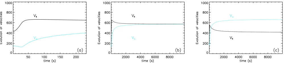
Another way to look at these results is presented in Fig.7, which shows the time evolution of the parallel (black) and per-pendicular velocities (blue) for the same particle orbits for which we showed the pitch angle evolution in Fig.6. The specific fea-ture we would like to point out in these plots is that the parallel velocity shows a rapid increase in the initial phase of each or-bit and then seems to reach a plateau or even drop offslightly, whereas the perpendicular velocity shows a more long-term evo-lution although it also levels offin the long run. However,v⊥ is often still increasing whenv has already either reached its plateau or is decreasing. Obviously, given the relation of the pitch angle with the components of the particle velocity, this sheds some additional light on the situation. We hypothesise at this point that these findings could at least partially be explained by the fact that while the motion of a field line slows down

considerably relatively early in the CMT evolution and Fermi acceleration thus basically stops, the field strength may still con-tinue to increase due to the effect of pile up of magnetic flux from above. We will explore this hypothesis further in Sect.4 below.

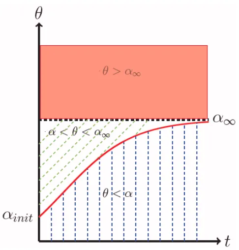
Generally, the situation we are facing with regards to es-cape or trapping of particle orbits in a CMT is summarised schematically in Fig.8. The red line indicates the time evolu-tion of the loss cone angleα(t). The loss cone angle generally increases from an initial valueαinit to an asymptotic valueα∞ ast→ ∞, although as mentioned above, this increase does not necessarily have to be monotonic. We have divided theθ-t-plane in the sketch tentatively into three regions: a region below the red curve representing the loss cone angleα(t) (hatched blue), a region above the asymptotic value of the loss cone angle,α_∞ (shaded brown) and the region between these two regions, where α(t)< θ(t)< α_∞(hatched green).

Fig. 5.Time evolution of the pitch angleθ(dotted black line) for particle orbits with initial pitch angles varying from 5◦to 19.6◦. Plota)andb) show the pitch angle evolution for the two orbits with initial pitch angles smaller than the inital loss cone angle of 11.8◦_{. Plotsc),e), andg)show}

Fig. 6.Long-term time evolution of the pitch angle for particle orbits with initial pitch angles 160.4◦(subcritical,a)), 159.0◦ (critical,b)), and 155.4◦(supercritical,c)). Due to the large number of bounces, only the maxima and minima of the pitch angle curves are shown for the particle orbit plotsb)andc). Particle orbits with subcritical angles escape, whereas particles with supercritical angles and above remain trapped.

Fig. 7.Subcriticala), criticalb), and supercriticalc)time evolution of parallel and perpendicular velocity for the particle orbits whose pitch angle evolution is shown in Fig.6. A key feature is thatv(black curves) reaches a plateau or even decreases slightly after an initial rapid increase, whilev⊥(blue) still continues to increase.

4. A discussion of trapping and escape using simplified models

In this section, we attempt to explain the previous results regard-ing the trappregard-ing and escape of particle orbits in a specific CMT model using some basic theoretical concepts. We will base our explanation on a simplified scenario for the acceleration within a CMT taking two features of particle orbits in CMTs found pre-viously byGrady et al.(2012) into account, namely:

1. increases in parallel velocity occur at the apex of field lines, 2. the position mirror points moves very little during the

evolu-tion of a CMT.

We remark that the second feature can only be satisfied approx-imately because otherwise no particle orbit would ever enter the loss cone. However, as we will see below, it is an approxima-tion that considerably simplifies the calculaapproxima-tions without aff ect-ing the conclusions too much.

Based on this, we simplify particle motion in a generic CMT in the way shown in the sketch in Fig.9. The particle orbit is represented by straight lines between the mirror points, which are kept at a fixed height, and the field line apex. The field line apex (loop top) moves downward at a speedvLT(t). The increase in parallel energy is modelled as an elastic bounce of the parti-cle offa “wall” moving with speedvLT(t) every time the particle orbit encounters the field line apex. We assume that the velocity remains constant between the bounces, so the simplified particle orbit consists of straight lines along which the particle moves with constant velocity. Simultaneously, we assume that the mag-netic field strength at the field line apex evolves according to a known functionB(t) and that the magnetic field strength at the footpoints, as well as their position remain constant. This allows

us to determine the time evolution of the loss cone angle for this simplified model as well as calculating the time development of the pitch angle at the field line apex just after a bounce.

The simplified model hence has the following ingredients:

– the loop top velocityvLT(t), which has to be specified as a function of time;

– the loop top magnetic field strength B(t), which has to be specified as a function of time;

– the initial height of the loop topyinit;

– the height of the mirror pointsymirror, which is assumed to be constant;

– the position of the foot points xinit, which is also assumed to be constant; this will be set indirectly by specifying the initial angleφinitof the particle orbit with the vertical. We also have to specify conditions for the initial velocityvinitand the initial pitch angleθinit. These ingredients can be condensed into a set of simple algebraic equations, which we present in AppendixA. These equations can be solved iteratively.

The main task is then to make sensible choices for vLT(t) andB(t). Obviously, guided by our CMT model discussed in Sect. 2, we generally want vLT(t) to be a function that de-creases with time and has an asymptotic value of zero andB(t) to be an increasing function of time with an asymptotic value of

Fig. 8.Sketch of the different regions in pitch angle vs. time evolution in a CMT. The red curve represents the time evolution of the loss cone angleα(t), which starts at a valueαinit and then increases with time towards an asymptotic valueα_∞. The blue hatched region represents the orbits with pitch angles less than the loss cone angle which are lost. Orbits with initial pitch angles greater thanα∞(brown shaded region) remain trapped (although see discussion in main text). For orbits with initial pitch betweenαinitandα∞(green hatched region) the outcome depends on the relative importance of Fermi vs. Betatron acceleration.

a way that the results resemble the numerical values of the par-ticle orbits calculated kinematic MHD CMT model shown in Sect. 3, one can only expect to recover the general behaviour of quantities like the pitch angle or the parallel and perpendic-ular velocity components in a qualitative way and one should not expect a numerically accurate representation of the full orbit calculations.

For our first combination (model 1) we make the simplest possible choice forvLT(t), which is to set it equal to a constant. To satisfy the condition that the asymptotic value ofvLT(t) as

t→ ∞should be zero, we assume thatvLT(t) drops to zero at a finite timetstop. In practice, we actually setvLT(t)=0 when the field line apex has decreased below a fixed heightymin, where ymin > ymirror. For this vLT(t), one can actually solve the al-gebraic equations presented in AppendixA analytically. This choice forvLT(t) is combined with aB(t) for which we have cho-sen an exponentially increasing model of the form

B(t)=B∞−B0 exp(−t/τ). (14) Instead of fixingB_∞andB0, we determine them from the val-ues ofBstart = B(0) andBfinal = B(tfinal), wheretfinalis the time at which we stop the simplified model calculation. The mirror height is determined from the initial pitch angle, according to Eq. (A.1), using f(θ)=cot0.1_{θfor this and the other two} simpli-fied models.

Some results for this simplified model are shown in Figs.10 and11. The values and parameters picked for this case were yinit = 4.2L,φinit = 15◦, Bstart/Bfp = 0.05, Bfinal/Bfp = 0.5, τ=0.4T, andvLT(t) =−4L/T. If we choose the same normal-isation as used byGiuliani et al.(2005) withL = 107_{m and}

Fig. 9.Sketch of the basic model used to explain the result found re-garding escape and trapping of particle orbits in CMTs.

T =100 s, we getτ=40 s andvLT(t)=−400 km s−1. The mag-netic field ratios imply that the initial loss cone angle has a value of 12.9◦and that the asymptotic loss cone angle is approximately 45◦. The time evolution of the pitch angle at the field line apex compared to the loss cone angle is shown in Fig.10for three different initial pitch angles with values of 22◦, 23◦, and 24◦. We selected these three values, because they straddle the critical ini-tial pitch angle, which divides trapping and escape for this par-ticular simplified model. In all three cases, we start with a pitch angle that is greater than the initial loss cone angle. In the case ofθinit =22◦, the curve of the pitch angle crosses into the loss cone, which means escape, whereas in the two other cases the pitch angle curves remain above the loss cone angle curve, al-beit only very slightly in the case ofθinit=23◦. One can see that the pitch angle initially increases, but then reaches a maximum and starts to decrease (this might be difficult to see in Fig.10, but one can check this numerically). This is the effect ofvLT(t) being non zero initially and thus Fermi acceleration becomes domi-nant at some point in this initial stage. AftervLT(t) drops to zero, betatron acceleration takes over and the pitch angle curves start increasing again.

In Fig.11, we show the time evolution of the parallel (black) and perpendicular velocities (blue) at the field line apex. The parallel velocity shows an initial increase during the time when vLT(t) is non-zero and after that it is constant. The perpendicular velocity increases on a longer timescale as it is only affected by the increase in magnetic field strength. Despite the extreme sim-plification of the acceleration process in this model both Figs.10 and11show features that are qualitatively similar to the features seen in Figs.6 and7. While this is reassuring let us first see whether this will be corroborated by the other two simplified models that we investigated.

Fig. 10.Evolution of loss cone α(red) and pitch angleθ(black) for a simplified CMT acceleration model (model 1) with constant loop top velocityvLT(t). Shown are the results for three different starting pitch anglesθi close to the critical initial pitch angle. One can see that both Fermi and Betatron accelerations are operating simultaneously, however, betatron acceleration is the overall dominating mechanism, causingθto increase.

Fig. 11.Time evolution ofv_⊥(blue) andv(black) for simplified model 1. The result for three different initial pitch anglesθiclose to the critical initial pitch angle are shown. One can see that the parallel velocity increases sharply in the initial phase while the loop top moves and stays constant after the loop top stops moving.

withv0 being the initial loop top velocity andτv the timescale on whichvLT(t) drops off. This timescale is not necessarily the same as the timescaleτon whichB(t) increases (see Eq. (14)), and we have chosenτ_v=0.144T andτ=0.25T(corresponding to 14.4 s and 25 s in theGiuliani et al. 2005normalisation). All initial conditions and theB-field ratios as well asφinithave been chosen to remain the same as for the first case. Because the loop top velocity is now exponentially decreasing, we have chosen its initial velocity to be higher than the constant velocity in model 1 withv0=−10 (=−1000 km s−1for the initial velocity).

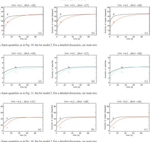
The results for model 2 are shown on Figs.12and13. We again show plots for cases with initial pitch angles close to the critical pitch angle defining the boundary between escape and trapping (θinit = 26◦, 27◦, and 28◦). The values of these initial pitch angles obviously differ from the values in model 1, because the time evolution of case 2 differs. Qualitatively, however, we again see similar features as in the full orbit calculations, with e.g.,v, showing a stronger increase at the beginning whenvLT(t) is large and then levelling off.

For the third case of a simplified model (model 3), we choose to take the functions given by Aschwanden (2004) for vLT(t) andB(t), but modify them slightly so that they match our de-sired model features. In particular, we assume that the asymp-totic B(t) as t → ∞ will be smaller than the footpoint field strength, whereasAschwanden(2004) assumes that they are the same, implying that the asymptotic loss cone angle approaches 90◦. We also start with a finite magnetic field strength, whereas Aschwanden’s model starts with vanishing field strength. In practice we achieve that by simply starting the model equations

at a finite time oft > 0. The loop top velocity functionvLT(t) actually has the same form as Eq. (15) and thus does not have to be changed. The loop top magnetic field strength is given by

B(t)=(B_∞−B0) sin2 _π

2

1−exp(−t/τ)+B0, (16) so that the magnetic field strength att =0 isB0and ast → ∞ we findB(t) → B_∞. We choose the same magnetic field ratios as for the two previous cases and also keepτvandτthe same as in case 2. Similarly, all other parameters and initial conditions remain unchanged.

Again, we show the results for three different values of the initial pitch angle in Figs.14and15. The three values (θi=27◦,

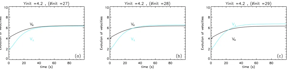
28◦, and 29◦) have been chosen such that they are in the region of values around the critical initial pitch angle, which is very close to 26◦. For this case, due to the modification of the time dependence ofB(t) there is an initial decrease in the pitch angle before it starts to increase in the later stages of the evolution. This is similar to what was found in model 1 for a later time. In model 2, the time evolution of the pitch angle differs because the magnetic field strengthB(t) increases exponentially fromt =0 on1_{. Model 3 again shows very similar qualitative features to our} kinematic MHD model results and to the other two simplified model cases.

Fig. 12.Same quantities as in Fig.10, but for model 2. For a detailed discussion, see main text.

Fig. 13.Same quantities as in Fig.11, but for model 2. For a detailed discussion, see main text.

Fig. 14.Same quantities as in Fig.10, but for model 3. For a detailed discussion, see main text.

to what we found from the guiding centre orbit calculations in Sect. 3. In particular, these findings seem to corroborate that there is a critical initial pitch angle below which particle orbits escape and above which particle orbits are trapped in a CMT. This critical initial pitch angle has a value, which is greater than the initial loss cone angle, but smaller than the asymptotic loss cone angle, and may vary from field line to field line. We have also confirmed that while Fermi acceleration may be dominat-ing in the initial phases of a particle orbit, betatron acceleration will take over at some point and thus generally the pitch angle will increase with time. Fermi acceleration and betatron acceler-ation in realistic CMTs will occur simultaneously and cannot be treated independently.

5. Summary and conclusions

We have presented a detailed investigation of the conditions that affect the trapping and escape of particle orbits in models of col-lapsing magnetic traps, starting with the investigation of guiding centre orbit calculations in the kinematic MHD CMT model of Giuliani et al.(2005). Based on the results of our investigations

and on observations made previously byGiuliani et al.(2005) and Grady et al.(2012), we designed a simplified schematic model for CMT particle acceleration and studied three different implementations of this schematic model, which all qualitatively corroborated the previous findings.

We showed that for each magnetic field line in a collapsing magnetic trap there is a critical initial pitch angle, which divides particle orbits into trapped orbits and escaping orbits. This crit-ical initial pitch angle is greater than the initial loss cone angle for the field line, but smaller than the value of the asymptotic loss cone angle for the field line ast→ ∞. We also investigated whether the critical initial pitch angle depends on the initial en-ergy of the particle, and we found that it does not.

Fig. 15.Same quantities as in Fig.11, but for model 3. For a detailed discussion, see main text.

efficiency of Fermi acceleration has to decrease on a particular field line during the time evolution of a CMT because the motion of the field line must slow down. On the other hand, the magnetic field strength can still continue to increase due to the pile-up of magnetic flux from above.

In the present paper, we have for simplicity excluded the pos-sibility of either Coulomb collisions, wave-particle interactions, or turbulence on the trapping or escape of particles from CMTs. Obviously, each of these mechanisms may change the results we have found in this paper. The effect of Coulomb collisions on particle acceleration in simple CMT models has been consid-ered byKovalev & Somov(2003),Karlický & Kosugi(2004), andBogachev & Somov(2009).Minoshima et al.(2011) have investigated the effects of pitch angle scattering by Coulomb col-lisions on trapping and escape, but without considering the effect of dynamical friction.Karlický & Bárta(2006) included the ef-fects of Coulomb collisions in their MHD model of a CMT. We also mention the recent paper byWinter et al.(2011), although a static field is used in that paper.

Obviously, wave-particle interaction and/or turbulence added to CMT model would also change both the energisation process and the pitch angle evolution of particle orbits in a col-lapsing magnetic trap. As already mentioned by Grady et al. (2012), a combination of a CMT model with stochastic accel-eration mechanisms (see, e.g., Miller et al. 1997) could pro-vide a link between those acceleration mechanisms and the stan-dard flare scenario along the lines proposed by e.g.,Hamilton & Petrosian(1992),Park & Petrosian(1995),Petrosian & Liu (2004), andLiu et al.(2008).

Acknowledgements. The authors would like to thank the referee for very

use-ful comments and acknowledge useuse-ful discussions with Eduard Kontar, Peter Cargill, Marian Karlicky, and Mykola Gordovskyy. This work was financially supported by the UK’s Science and Technology Facilities Council.

Appendix A: Simplified model: mathematical description

We assume here that the functionsvLT(t) and B(t) are known. In the coordinate system used,vLT(t) should be negative as the height of the field line apex should decrease in time.B(t) should be a function that increases with time. For both functions, obvi-ously many different choices are possible and we therefore im-posed the additional condition of simplicity on the functions.

As discussed in the main text, we make the simplifying as-sumption that the mirror height of each particle orbit is fixed. Without a detailed magnetic field model and an explicit calcula-tion of the corresponding particle orbits (which is exactly what we want to avoid in our simplified model), we can only choose an ad hoc position of the mirror height. We know, however, that

the mirror height should be coupled with the value of the initial pitch angle of a particle orbit and that the mirror height should decrease with a decrease of the initial pitch angle, with the mir-ror height eventually reaching zero (lower boundary) when the initial pitch angleθinitis equal to the initial loss cone angleαinit. This relation can be parametrized as:

ymirror=yinit

1− f(θinit)

f(αinit)

, (A.1)

wheref(θ) is a function, which monotonically increases from a value of 0 atθ=90◦. In this paper, we have chosenf(θ)=cotq_θ,

withq>0 a real parameter, but other choices are, of course, also possible.

The simplified model can be completely expressed in terms of motion in they-direction and all other quantities can be de-rived from that. We start by imagining the state of the system just after the particle has bounced offthe field line apex for theith time. Let the time of the bounce betiand the positionyi=y(ti).

The velocity of the particle orbit in they-direction then has the valuev_y,i. The particle will then move down to the mirror point

with this velocity, bounce offthe mirror point without chang-ing the absolute value of its velocity (it is at this point that the assumption of the mirror points being static simplifies matters enormously) and move back up to the field line apex for the next bounce offthe loop top at timeti+1. During that bounce thevy -component of the velocity will change to

vy,i+1=vy,i+2vLT(ti+1). (A.2) The particle will have travelled a total distance ofyi₊1 +yi−

2ymirror (distance down plus distance up) in the timeti+1 −ti,

leading to the equation

yi+1=−yi+2ymirror+(ti+1−ti)vy,i. (A.3)

On the other hand, because the field line apex is moving with velocityvLT(t), we also have

yi+1=yi+ ti+1

ti

vLT(t) dt=yi+Fy(ti+1)−Fy(ti) (A.4)

withF_y(t)= vLT(t)dt. We would like to point out that the time

ti+1of the next bounce is unknown and has to be calculated. This can be done by combining Eqs. (A.3) and (A.4) to elim-inate the equally unknownyi₊1to get the transcendental equation

method. However, for the case of a constantvLT(t) the equation becomes linear and can be solved analytically.

Onceti+1 is known, all other relevant quantities can be de-termined and the process can be repeated until the end of the calculation.

References

Aschwanden, M. J. 2004, ApJ, 608, 554

Bogachev, S. A., & Somov, B. V. 2005, Astron. Lett., 31, 537 Bogachev, S. A., & Somov, B. V. 2009, Astron. Lett., 35, 57 Giuliani, P., Neukirch, T., & Wood, P. 2005, ApJ, 635, 636

Grady, K. J. 2012, Ph.D. Thesis, University of St Andrews, St Andrews, UK Grady, K. J., & Neukirch, T. 2009, A&A, 508, 1461

Grady, K. J., Neukirch, T., & Giuliani, P. 2012, A&A, 546, A85 Hamilton, R. J., & Petrosian, V. 1992, ApJ, 398, 350

Karlický, M., & Bárta, M. 2006, ApJ, 647, 1472

Karlický, M., & Kosugi, T. 2004, A&A, 419, 1159 Kovalev, V. A., & Somov, B. V. 2003, Astron. Lett., 29, 409 Krucker, S., Battaglia, M., Cargill, P. J., et al. 2008, A&ARv, 16, 155 Liu, W., Petrosian, V., Dennis, B. R., & Jiang, Y. W. 2008, ApJ, 676, 704 Miller, J. A., Cargill, P. J., Emslie, A. G., et al. 1997, J. Geophys. Res., 102,

14631

Minoshima, T., Masuda, S., & Miyoshi, Y. 2010, ApJ, 714, 332

Minoshima, T., Masuda, S., Miyoshi, Y., & Kusano, K. 2011, ApJ, 732, 111 Northrop, T. G. 1963, The Adiabatic Motion of Charged Particels (New York:

Wiley)

Park, B. T., & Petrosian, V. 1995, ApJ, 446, 699 Petrosian, V., & Liu, S. 2004, ApJ, 610, 550

Somov, B. V. 2004, in Multi-Wavelength Investigations of Solar Activity, eds. A. V. Stepanov, E. E. Benevolenskaya, & A. G. Kosovichev, IAU Symp., 223, 417

Somov, B. V., & Bogachev, S. A. 2003, Astron. Lett., 29, 621 Somov, B. V., & Kosugi, T. 1997, ApJ, 485, 859