Title & running title: Distance sampling with camera traps 1
Word count (excluding this page):6998 2
Authors: Eric J. Howe1*, Stephen T. Buckland1, Marie-Lyne Després-Einspenner2, Hjalmar S. 3
Kühl2, 3 4
5
1 Centre for Research into Ecological and Environmental Modelling, University of St Andrews, 6
The Observatory, Buchanan Gardens, St Andrews, Fife KY16 9LZ, UK 7
2 Max Planck Institute for Evolutionary Anthropology, Deutscher Platz 6, 04103, Leipzig, 8
Germany 9
3 German Centre for Integrative Biodiversity Research (iDiv) Halle-Jena-Leipzig, Deutscher 10
Platz 5e, 04103 Leipzig, Germany 11
* Correspondence author. E-mail: [email protected] 12
Summary 14
1. Reliable estimates of animal density and abundance are essential for effective wildlife 15
conservation and management. Camera trapping has proven efficient for sampling multiple 16
species, but statistical estimators of density from camera trapping data for species that cannot be 17
individually identified are still in development. 18
2. We extend point-transect methods for estimating animal density to accommodate data from 19
camera traps, allowing researchers to exploit existing distance sampling theory and software for 20
designing studies and analyzing data. We tested it by simulation, and used it to estimate 21
densities of Maxwell’s duikers (Philantomba maxwellii) in Taï National Park, Côte d’Ivoire. 22
3. Densities estimated from simulated data were unbiased when we assumed animals were not 23
available for detection during long periods of rest. Estimated duiker densities were higher than 24
recent estimates from line transect surveys, which are believed to underestimate densities of 25
forest ungulates. 26
4. We expect these methods to provide an effective means to estimate animal density from 27
camera trapping data and to be applicable in a variety of settings. 28
29
Keywords: animal abundance, camera trapping, density, distance sampling, Maxwell’s duiker 30
31
Introduction 32
Remote motion-sensitive photography, or camera trapping, is increasingly used in 33
wildlife research, and allows multiple research objectives to be addressed (Sollmann et al. 2013a, 34
Burton et al. 2015, Rovero and Zimmermann 2016). Estimation of population density (𝐷) is a 35
camera traps (Burton et al. 2015, Rovero and Zimmermann 2016). If individuals are 37
recognizable, density can be estimated using spatially explicit capture–recapture (SECR) models 38
(Efford et al. 2009), but methods for estimating D from camera trapping data in the absence of 39
individual identification are still in development (Sollmann et al. 2013a, Burton et al. 2015, 40
Dénes et al. 2015, Rovero and Zimmermann 2016). Detection rates at camera traps have been 41
used to index abundance, but indices can rarely be converted to estimates of absolute density, 42
and spatiotemporal variation in detection rates does not provide reliable evidence of differences 43
or trends in abundance (Sollmann et al. 2013b, Burton et al. 2015). The random encounter 44
model (REM) estimates absolute density as a function of the detection rate, the dimensions of a 45
sector within which detection is certain, and the speed of animal movement; methods for 46
quantifying the latter two parameters from camera trapping data have been described (Rowcliffe 47
et al. 2008, 2011, 2016). The REM has been recognized as a potentially useful model, but its 48
accuracy and reliability remains to be demonstrated (Rovero and Marshal 2009, Sollmann et al. 49
2013a, Zero et al. 2013, Cusack et al. 2015a, Balestrieri et al. 2016, Caravaggi et al. 2016). 50
SECR estimators for unmarked populations estimate the number and location of animals’ activity 51
centers from the spatial correlation of counts at different sampling locations; sampling must be 52
sufficiently intensive to detect the same animals at multiple locations, and estimates lack 53
precision (Chandler and Royle 2013). 54
Here we describe how densities of unmarked animal populations can be estimated by 55
distance sampling (DS) with camera traps, allowing researchers to take advantage of a well-56
described theoretical framework complete with software and advice for designing studies and 57
analyzing data (Buckland et al. 2001, 2004, 2015, Thomas et al. 2010, Miller 2015, 58
camera traps and describe its assumptions and the estimation of variances. We test for bias in 60
estimated density (𝐷̂) and its variance by simulation, and apply the method to estimate the 61
density of Maxwell’s duikers (Philantomba maxwellii) in Taï National Park, Côte d’Ivoire. 62
63
Methods 64
Formulation of the Model 65
A camera trap (CT) is deployed at a point 𝑘 that is independent of animal density for a 66
period of time 𝑇𝑘 and set to record images for as long as an animal is present to trigger it. We 67
predetermine a finite set of snapshot moments within Tk, t units of time apart, at which an image
68
of an animal could be obtained. Temporal effort at the point is then Tk / t. When images of
69
animals are obtained, we estimate the horizontal radial distance 𝑟𝑖 between the midpoint of each 70
animal and the camera, at each snapshot moment, for as long as it remains in view. If the camera 71
covers an angle θ radians, then 2𝜋𝛳 describes the fraction of a circle covered by the camera, so we 72
define overall sampling effort at point 𝑘 as 𝜃𝑇𝑘
2𝜋𝑡. We regard the data as a series of snapshots, and
73
density estimation follows by standard point transect methods (Buckland et al. 2001). We 74
estimate 𝐷 as 75
𝐷̂ = ∑𝐾𝑘=1𝑛𝑘 𝜋𝑤2∑ 𝑒
𝑘𝑃̂𝑘 𝐾
𝑘=1 (1)
76
where 𝑒𝑘 =𝜃𝑇𝑘
2𝜋𝑡 is the effort expended at point 𝑘, 𝐾 is the set of points, 𝜃 is the horizontal angle
77
of view (AOV) of the camera, 𝑤 is the truncation distance beyond which any recorded distances 78
are discarded, nk is the number of observations of animals in the population of interest at point k,
79
and 𝑃̂𝑘 is the estimated probability of obtaining an image of an animal that is within θ and w in 80
. Substituting 𝑒𝑘 in (1), we have
82
𝐷̂ = 2𝑡 ∑𝐾𝑘=1𝑛𝑘 𝜃𝑤2∑ 𝑇
𝑘𝑃̂𝑘 𝐾
𝑘=1 (2)
83
We use the distances 𝑟𝑖 to model the detection function and hence to estimate 𝑃𝑘. 84
85
Assumptions and Practical Considerations 86
The usual DS assumptions apply (see Chapter 2 of Buckland et al. 2001). We record 87
distances at instantaneous snapshot moments to ensure that animal movement does not bias the 88
distribution of detection distances. Below, we describe an approach for accurately assigning 89
animals to distance intervals; Rowcliffe et al. (2011) and Caravaggi et al. (2016) describe 90
methods for measuring continuous distances between CTs and detected animals. 91
Random designs or systematic designs with random origin are consistent with the 92
assumption that points are placed independently of animal locations. Selecting camera 93
orientations as part of the design is also advisable. Orientations could be selected randomly, or 94
the same orientation could be used for all cameras. Deviating slightly from the location and 95
orientation selected by design (e.g., to attach the camera to a nearby tree or to avoid an obscured 96
field of view) would not bias estimates provided field staff do not intentionally target habitat 97
features known to be either preferred or avoided by the animals. 98
Empirical, design-based estimators of the encounter rate variance are robust to violation 99
of the assumption that detections are independent events (Fewster et al. 2009, Buckland et al. 100
2015). However, in CT surveys we expect violations to be severe because we include multiple 101
detections of the same animal during a single pass through the detection zone. We can avoid this 102
assumption by estimating variances using a nonparametric bootstrap, resampling points with 103
independence is that the usual goodness-of-fit tests and model selection criteria are invalid 105
(Buckland et al. 2001). Methods for selecting among DS models when observations are not 106
independent are in development. 107
The assumption that detection is certain at zero distance could be violated by (1) animals 108
passing beneath the field of view (FOV) of the camera, (2) failure to identify the species because 109
only part of the animal is visible, and possibly (3) the delay between the time the sensor is 110
activated and the time the first image is recorded (the “trigger speed”), if animals directly in front 111
of the camera at a snapshot moment do not yield images. Such violations may be detectable 112
during exploratory analysis in the form of fewer than expected detections near the point, and bias 113
can be avoided via left-truncation (Buckland et al. 2001, Marques et al. 2007, e.g. Obbard et al. 114
2015). To minimize violations and ensure that detection probability is certain or high at some 115
distance near the point, cameras should be set at a height appropriate to the species of main 116
interest (Rovero and Zimmermann 2016). Lower heights would reduce the chance of small 117
animals passing beneath the camera at short distances, but would also reduce the range of 118
distances over which animals could be detected and therefore sample size and flexibility when 119
modelling the detection function. Pairs of CTs triggered by passive infrared (PIR) sensors and 120
mounted at the same location, height, and orientation, or one PIR CT deployed in combination 121
with other sampling devices (track plots, CTs triggered by pressure plates or active IR sensors) 122
could facilitate field tests of whether or not detection probability is close to 1 at short distances in 123
front of PIR CTs. Paired cameras mounted some distance apart targeting the same location 124
would not provide an effective test, but would provide the data needed to apply mark–recapture 125
distance sampling methods, which avoid this assumption (Buckland et al. 2004, Laake et al. 126
In traditional point transect surveys, human observers measure distances to each detected 128
animal only once during each visit to a point, and effort at each point is the number of times it 129
was visited. CTs remain at the point, but the snapshot approach discretizes the number of times 130
we could potentially detect each animal (as Tk / t as described above). However, CTs detect only
131
moving animals within the range of the sensor and the FOV of the camera, and can be 132
programmed to record multiple still images, or video footage, each time the sensor is triggered 133
(Rovero and Zimmermann 2016). These characteristics of CTs as observers must be taken into 134
consideration. Observed distances upon first detection are expected to be positively biased 135
because animals entering the detection zone through the arc of the sector would contribute a 136
disproportionate number of observations at far distances. Bias would be slight if the time 137
between snapshot moments (t) was small enough to ensure that the animals did not move far 138
relative to the range of the sensor between snapshots, as then the observations would be 139
representative of animals’ continuous paths past the CTs. However, we prefer to avoid the 140
potential for bias by assuming that the snapshot moments are selected independently of animal 141
locations, and predetermining them as specific times of day to ensure that the assumption is met. 142
Practical considerations constrain t. If t is large, animals that trigger the sensor might leave the 143
detection zone before a snapshot moment arises, which would not cause bias but wastes data. As 144
t is reduced, there would be fewer missed detections and larger samples as we record distance to 145
each animal multiple times during a single pass in front of the CT. Eventually, improvements in 146
the precision of 𝐷̂ with larger samples would become negligible because variation in the 147
encounter rate among points would contribute most of the variation in estimated density. 148
Reducing t further would then needlessly increase the time required to process and analyze the 149
lower end of the range being more appropriate for faster-moving or rarer animals, and CTs with 151
faster trigger speeds. 152
Programming cameras to record time-stamped video would make it straightforward to 153
record distances at the predetermined snapshot moments. If still images are preferred, cameras 154
should be programmed to record an image at the next several snapshot moments when triggered, 155
or, if this is not feasible, to record a rapid series or “burst” of still images to ensure that images 156
are recorded at times that align with snapshot moments. There should always be the potential for 157
the camera to be triggered again immediately or after a minimal delay. Note that depending how 158
cameras are programmed, the sample of distances observed in CT data may or may not comprise 159
a realization from the detection function described by the probability that an animal at distance r 160
triggers the sensor. If cameras record a single image at the subsequent snapshot moment, or a 161
rapid series of images for < t seconds, when the sensor is triggered, then each detection of an 162
animal that triggers the sensor several times during a pass in front of a CT is a function of the 163
sensitivity of the sensor. If cameras are set to record video, or a series of still images for > 2t 164
seconds, then all but the first detection is certain for as long as the animal remains in the FOV 165
and the camera continues to record images. Furthermore, regardless of how the camera is 166
programmed, any other animals in the FOV while the camera is recording images would 167
contribute observations that do not depend on the sensitivity of the sensor. These differences do 168
not invalidate the method provided we define the detection function as representing the 169
proportion of locations at different distances which are recorded, regardless of whether an animal 170
triggered the sensor at that distance. 171
Obviously, we can only estimate the density of populations that are available for 172
detection by CTs. Similarly, because the sampling duration at each location (𝑇𝑘) is part of the
model definition, we expect densities of animals that spend part of their time outside the vertical 174
range of camera traps to be underestimated, and for the bias to be proportional to time animals 175
are not available for detection. For example, with 𝑇𝑘 set to the study duration, we expect 𝐷̂ of a
176
species that spends all its time in the canopy to be zero, and of a species that spends half its time 177
underground and the rest at ground level to be half of the true density. Negative bias would also 178
result if animals went undetected only because movement was insufficient to trigger the sensor. 179
To avoid this bias, either 𝑇𝑘 should be defined as the amount of time that the entire population
180
was available for detection while cameras were operating, or, equivalently, the proportion of 181
time when animals were available for detection should be included as a parameter in the model. 182
Animals are unavailable for detection when outside the vertical range of CTs, and may not be 183
available when within this range depending on their level of activity. We explore this issue 184
further in subsequent sections. 185
186
Simulations 187
We tested the method using simulations employing simple and complex models of animal 188
movement and different sampling scenarios (see supplemental material). With the simple model, 189
animals moved continuously at a constant speed and tended to maintain their heading. The 190
complex model included variable speeds and tortuosities, and all animals rested for the same 12 191
hours of each day. We recorded the distance between cameras and animals within detection 192
zones every two seconds, 24 hours per day. Where the complex model was used, we also 193
collected data only when animals were moving, and reduced Tk by half accordingly when
194
estimating density. 195
Example: Maxwell’s duikers in Taï National Park 197
We used point transect DS methods to estimate the density of Maxwell’s duikers within 198
the territory of the “east group” habituated chimpanzee community in Taï National Park, Côte 199
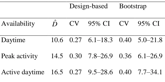
d’Ivoire (Després-Einspenner et al. accepted; Fig 1a). Maxwell’s duikers were sampled from 28-200
June through 21-Sept, 2014 at 23 camera traps (Bushnell Trophy CamTM; Model 119576C) 201
mounted at a height of 0.7 – 1.0 m and set to high sensitivity. Cameras were deployed with a 202
fixed orientation of 0˚ at the intersections of a grid with 1 km spacing and a random origin 203
superimposed over the study area (Fig. 1b). Realized sampling locations and orientations 204
deviated from the design by as much as 30 m, and 40˚, respectively, in order to mount cameras 205
on trees and to ensure there was some chance of detecting animals. During installation of each 206
camera, we measured horizontal radial distances from the camera, and recorded videos of 207
researchers holding distance markers, at 1 m intervals out to 15 m, in the center and along both 208
sides of the FOV. We estimated distances to filmed duikers by comparing their locations to 209
those of researchers in the reference videos. We set t = 2 seconds, and recorded the distance 210
interval within which the midpoint of each animal fell at 0, 2, 4, … , 58 seconds after the minute. 211
Larger distances were more difficult to measure precisely, so we assigned animals to 1-m 212
intervals out to 8 m, but binned observations between 8 and 10 m, 10 and 12 m, 12 and 15 m, 213
and beyond 15 m. 214
We excluded data from one camera because the FOV was largely obscured by vegetation, 215
and another which was placed on a slope and failed to detect any animals, but we included data 216
from a third camera that functioned normally but did not detect any duikers. Maxwell’s duikers 217
sleep or rest for most of each night and for shorter periods during the day (Newing 1994, 2001). 218
darkness (19:00 – 6:00) from Tk a-priori. We accounted for limited availability during the
220
daytime three different ways. First we naively assumed that all duikers were active by 6:30:00 221
and remained so through 17:59:59, included distances observed during this interval in a 222
“daytime” data set, and defined temporal effort at each location (Tk / t) as the number of
2-223
second time steps during that time interval (20699), multiplied by the number of sampling days. 224
Second, we assumed that all animals were available only during apparent times of peak activity 225
(6:30:00 – 8:59:59 and 16:00:00 – 17:59:59) and recalculated temporal effort and censored 226
distance observations accordingly (Tk / t per day = 8098). Third, we defined Tk and included
227
observations as above for the daytime data set, and included an independent estimate of the 228
proportion of time captive Maxwell’s duikers were active during the same time interval (0.64; 229
Newing et al. 2001) in the denominator of Eq. 2. We included only data from complete days 230
when cameras were operating and not visited by researchers. 231
We fit point transect models in program Distance (version 7.0; Thomas et al. 2010), 232
defining survey effort at each location as 𝜃𝑇2𝜋𝑡𝑘. The cameras had an AOV of 42˚, and a wider 233
effective angle of the sensor (Trailcampro.com 2015), so we set θ = 42˚ or 0.733 radians. We 234
considered models of the detection function with the half-normal key function with 0, 1 or 2 235
Hermite polynomial adjustment terms, the hazard rate key function with 0, 1, or 2 cosine 236
adjustments , and the uniform key function with 1 or 2 cosine adjustments. Adjustment terms 237
were constrained, where necessary, to ensure the detection function was monotonically 238
decreasing. We selected among candidate models of the detection function by comparing AIC 239
values, acknowledging the potential for overfitting because many observations were not 240
Fewster et al. 2009, Web Appendix B), and from 999 bootstrap resamples, with replacement, 242
across camera locations. 243
244
Results 245
Simulations 246
Where we used the simple model of animal movement, and where we used the complex 247
model of animal movement and collected data only when animals were active, Dˆ was unbiased 248
(Table S1). Results were biased and erratic when we recorded distances to resting animals (see 249
supplemental material for details). Design-based variances were smaller than the sampling 250
variance of 𝐷̂ across iterations, and associated confidence interval coverage was <90% (Table 251
S1). Where we estimated variance by bootstrapping, the coefficient of variation was 0.119, 252
similar to the sampling variance of 𝐷̂, and CI coverage was 93.6% across 1000 iterations. 253
Doubling spatial sampling effort improved precision, slightly more so where we doubled the 254
number of locations as opposed to 𝜃 (Table S1). 255
256
Example: Maxwell’s duikers in Taï National Park 257
We obtained 11324 observations of the distance between Maxwell’s duikers and cameras 258
in 806 different videos. Duikers were rarely filmed during hours of darkness. The frequency of 259
detection increased steadily after 6:00 to a maximum between 6:30 and 7:00 and remained 260
relatively high until 9:30, after which it decreased slightly and remained relatively low until 261
16:30, then increased again and remained high until 18:00, then declined gradually until 19:00 262
asleep or stationary for an entire minute. We recorded 11180 distances from 6:30:00 through 264
17:59:59, and 6274 during times of peak activity. 265
Exploratory analyses revealed no evidence of data collection errors, and a paucity of 266
observations between 1 and 2 m but not between 2 and 3 m, so we left-truncated at 2 m. Fitted 267
detection functions and probability density functions were heavy-tailed when distances > 15 m 268
were included, so we right-truncated at 15 m. Truncating removed 8% of observations from the 269
daytime data set, leaving n = 10284, and 6.5% of observations from the peak activity data set, 270
leaving n = 5865. Mean encounter rates (mean numbers of duikers observed per 2-second time 271
interval) across all points were 3.27 × 10⁻⁴ during the daytime and 4.76 × 10⁻⁴ during times of 272
peak activity. Encounter rates were highly variable among locations but did not exhibit an 273
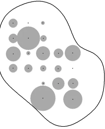
obvious spatial pattern across the study area, and there was no evidence of spatial autocorrelation 274
(Moran’s I P = 0.47; Fig. 3). 275
When we fit the hazard rate model with two adjustment terms to the daytime data set, the 276
detection function was not monotonically decreasing, so this model was not considered for 277
estimation. All models were fitted successfully to the peak activity data set. The hazard rate 278
model with no adjustments minimized AIC and was used to estimate density in both cases. 279
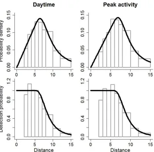
Probability density functions of observed distances and relationships between detection 280
probability and distance were similar (Fig. 4). Detection probability was ~1.0 within 5 m and 281
0.05 at 15 m; effective detection radii were 9.1 and 9.4 m from the daytime and peak activity 282
data sets, respectively. 283
We expected to underestimate density where we assumed duikers were active all day; 𝐷̂ 284
was 37% higher when we included only data from times of peak activity (Table 1). Including an 285
model fit to the daytime data set yielded a still higher estimate (“Active daytime” in Table 1). 287
Measures of uncertainty in the proportion of time active were not available (Newing et al. 2001) 288
so did not contribute to the variance of 𝐷̂. Bootstrap variances were larger than design-based 289
analytic variances (Table 1). The vast majority (99.8%) of the design-based variance of 𝐷̂ was 290
attributable to the variation in encounter rate between locations, and only 0.2% to detection 291
probability. 292
293
Discussion 294
Simulations demonstrated the potential for the method to yield unbiased density 295
estimates, but also that animals’ activity patterns must be accounted for. Where simulated 296
animals rested for half of each day and we set Tk equal to the survey duration, the most common
297
scenario was that animals did not rest in front of CTs and negative bias in 𝐷̂ was proportional to 298
the time spent resting. When we recorded distance at each snapshot moment while animals 299
rested in front of CTs, the encounter rate and therefore 𝐷̂ was higher on average, but the shape of 300
the detection function was strongly affected, leading to erratic estimates and cases where models 301
could not be fitted to the data. In practice, it is unlikely that we would detect animals while they 302
sleep or rest because movement will be insufficient to trigger the sensor. Therefore, estimates of 303
the proportion of time animals are active within the vertical range of CTs will be required to 304
avoid negatively biased 𝐷̂. Ideally, this proportion would be estimated from data collected 305
concurrently with the distance data to ensure it is representative. Fortunately, the temporal 306
distribution of camera trap detections is informative regarding animal activity patterns (Lynam et 307
al. 2013, Cruz et al. 2014, Rowcliffe et al. 2014). If it is reasonable to assume that the entire 308
required to estimate 𝐷̂ accurately, because we could either (1) analyze only the data collected at 310
that time, censoring effort and distance data from other times, or (2) estimate the overall 311
proportion of time active directly from the CT data (e.g. Rowcliffe et al. 2014). Newing’s (1994) 312
data from Taï indicated that there was no time at which all wild duikers could be assumed to be 313
active. If this was true during our survey, we may have underestimated density where we did not 314
correct for limited availability within the time included in Tk, because even at times of peak
315
activity some animals may have been resting and unavailable for detection. Activity data from 316
wild duikers were presented only as figures and could not be converted into estimates of the 317
overall proportion of time active (Newing 1994). We therefore relied on the assumption that 318
activity data from captive duikers (Newing 1994, Newing et al. 2001) were representative of 319
activity patterns during our survey. If this assumption held, then the density estimate calculated 320
using their estimate of the proportion of time active during the day should not be biased as a 321
result of limited availability. We suggest that the need to account for availability should not pose 322
a serious obstacle to reliable estimation of the density of many species, but for others, notably 323
ectotherms, and semi-arboreal and fossorial species, it will require careful consideration, and 324
possibly additional data. We further suggest that combining Rowcliffe et al.’s (2014) or similar 325
methods for estimating the proportion of time active from detection times at CTs with the point 326
transect method described here could yield accurate density estimates for many species from CT 327
data alone. 328
Avoidance of, or attraction to, CTs would bias encounter rates and therefore density 329
estimates. Some species exhibit complex responses to CTs or are particularly wary of humans 330
(Séquin et al. 2003). If behavioural responses are expected or apparent in images of detected 331
accustomed to them and for signs of human presence to dissipate. Similarly, effort and distance 333
data from times when animals may have been displaced from the trap sites by humans visiting 334
them to download data, replace batteries, etc., should be censored. 335
The probability of detection at PIR CTs is lower at greater angles from the center of the 336
FOV, due to a combination of the trigger speed, the effective horizontal angle of the sensor 337
relative to the AOV of the camera (which varies among CT models) and possibly reduced 338
sensitivity of the sensor at the periphery of its horizontal range (Rowcliffe et al. 2011, Rovero et 339
al. 2013, Rovero and Zimmermann 2016). This introduces heterogeneity in the detection 340
function. Fortunately, provided that detection is certain at zero distance, the pooling robustness 341
property ensures that estimation is unbiased in the presence of heterogeneity in detectability 342
among individuals (Buckland et al. 2004), and this also applies to heterogeneity caused by 343
differences in angle at different snapshot moments. However, if detection probability at high 𝜃 344
is much lower than in the centre, fitted models of the detection function might show a rapid drop 345
in detection probability near the point, whereas detection functions with a gradual decrease near 346
the point are preferred for stable density estimation (Buckland et al. 2001). The expected 347
distribution of angles within a sector within which the sensor is fully effective is uniform. We 348
recommend that researchers measure angles as well as distances to detected animals (e.g. 349
Carravaggi et al. 2016), and test for departures from the uniformity assumption at increasing 350
angles as part of their exploratory analysis. If departures are apparent, the data could be 351
truncated to exclude observations beyond an angle within which the distribution is approximately 352
uniform, in which case 𝜃 should be set to two times the truncation angle rather than the AOV of 353
the camera in the definition of effort. An alternative approach that would allow us to retain all of 354
depends on both radial distance and angle from center, using methods similar to those developed 356
by Marques et al. (2010). We expect heterogeneity with angle to be more severe with CT 357
models with narrow horizontal ranges of the sensor relative to the AOV of the camera, or slow 358
trigger speeds, and where faster-moving animals are sampled. CTs with fast trigger speeds, short 359
recovery times, and curved array Fresnel lenses (which provide a wide effective angle of 360
detection such that the camera begins recording images as or even before the animal enters the 361
FOV; Rovero and Zimmermann 2016) could reduce or eliminate differences in detection 362
probability at different angles in future studies. 363
The encounter rate variance accounted for the vast majority of the design-based variance 364
in duiker density, and variances around 𝐷̂ were larger than for simulated data despite similar 365
sample sizes. Real populations exhibit clumped or patchy distributions and non-random 366
movement, leading to variable encounter rates among sampling locations and hence greater 367
uncertainty in 𝐷̂ (Buckland et al 2001, Fewster et al. 2009); the small area sampled at each 368
location exacerbates this problem. Increasing the area sampled will therefore enhance precision, 369
more so than would increasing temporal effort at a point. Theory predicts that increasing the 370
number of points will yield the largest improvements to precision (Buckland 1984, Fewster et al. 371
2009). That the improvement in precision in simulations was only slightly greater where we 372
doubled the number of sampling locations than where we doubled 𝜃 is not representative of real 373
studies because the expected spatial distribution of animal locations was uniform, and movement 374
was random. Coefficients of variation around 𝐷̂ for duikers were >35% despite large samples of 375
distance observations, so we recommend that future studies employ more points to improve 376
The density of Maxwell’s duikers at Taï was recently estimated as 1.6 / km2 from line 378
transect DS surveys (N’Goran 2006). However, line transect sampling by human observers is 379
believed to severely underestimate densities of forest-dwelling animals in general, and forest 380
antelopes in particular, due to effects of evasive movement and behaviour in response to 381
observers on both the encounter rate and the distribution of observed distances (Koster and Hart 382
1988, Jathanna et al. 2003, Rovero and Marshall 2004, 2009, N’Goran 2006, Marshall et al. 383
2008, Marini et al. 2009). Estimates of sign density from line transect surveys are frequently 384
converted to estimates of animal density, but this is expected to yield biased estimates in the 385
absence of local and concurrent estimates of sign production and decay rates, which are time-386
consuming to estimate (Plumptre 2000, Kuehl et al. 2007, Todd et al. 2008). Dung surveys may 387
further require genetic analysis to identify the species (Bowkett et al. 2009). Distance sampling 388
with CTs apparently avoided the underestimation characteristic of line transect surveys of live 389
animals, in less time than would be required to obtain reliable estimates from sign surveys. 390
The recent proliferation of CT studies is providing new information about wildlife in 391
diverse habitats (Burton et al. 2015, Rovero and Zimmermann 2016). Where estimating the 392
density of a rare but individually identifiable species is the primary research objective, it may be 393
preferable to deploy CTs non-randomly in order to obtain sufficient detections of individuals to 394
estimate density by SECR (Wearn et al. 2013, Cusack et al. 2015b, Després-Einspenner et al. 395
accepted). However, multiple research objectives can be addressed, and useful data for multiple 396
species obtained, if CTs are deployed according to a randomized design (MacKenzie and Royle 397
2005, Wearn et al. 2013, Burton et al. 2015, Dénes et al. 2015). The size of unmarked 398
populations can then be estimated from CT data using Poisson and negative binomial GLMs or 399
because it is more biologically relevant and comparable across studies. Densities of unmarked 401
animal populations can only be estimated from CT data using SECR models for unmarked 402
populations, the REM, or DS methods; the latter two require randomized designs (Rowcliffe et 403
al. 2008, Buckland et al. 2001). SECR methods for unmarked populations require intensive 404
designs, and even then estimates will often be too imprecise to be useful unless a subset of the 405
population can be reliably identified (Chandler and Royle 2013, Saout et al. 2014). The REM 406
requires an estimate of the average speed of animal movement, assumes that detection is certain 407
within an estimable area in front of the camera, and makes use of only one observation from each 408
detected animal (Rowcliffe et al. 2008). Our point transect approach requires an estimate of the 409
proportion of time animals are available for detection, assumes that detection is certain only at 410
zero distance, and multiple observations from each detected animal inform detection probability 411
estimates. We expect the extension of point transect DS methods to provide an effective and 412
efficient tool for estimating animal density and to enhance the information derived from CT 413
surveys. 414
415
Acknowledgements 416
We thank the Robert Bosch Foundation, the Max Planck Society, and the University of St 417
Andrews for funding, the Ministère de l'Enseignement Supérieur et de la Recherche Scientifique 418
and the Ministère de l’Environnement et des Eaux et Forêts in Côte d’Ivoire for permission to 419
conduct field research in Taï National Park, and Dr. Roman Wittig for permitting data collection 420
in the area of the Taï Chimpanzee Project. 421
422
Balestrieri A, Ruiz-González A, Vergara M, Capelli E, Tirozzi P, Alfino S, Minuti G, Prigioni C, 424
Saino N. 2016. Pine marten density in lowland riparian woods: a test of the Random Encounter 425
Model based on genetic data. Mammalian Biology-Zeitschrift für Säugetierkunde 426
doi:10.1016/j.mambio.2016.05.005 427
428
Bowkett AE, Plowman AB, Stevens JR, Davenport TR, van Vuuren BJ. 2009. Genetic testing of 429
dung identification for antelope surveys in the Udzungwa Mountains, Tanzania. Conservation 430
Genetics 10:251-255 431
432
Buckland ST. 1984. Monte Carlo confidence intervals. Biometrics 1:811-817 433
434
Buckland ST, Anderson DR, Burnham KP, Laake JL, Borchers DL, Thomas L. 2001. 435
Introduction to distance sampling: estimating abundance of biological populations. Oxford 436
University Press, Oxford 437
438
Buckland ST, Anderson DR, Burnham KP, Laake JL, Borchers DL, Thomas L. 2004. Advanced 439
distance sampling: estimating abundance of biological populations. Oxford University Press, 440
Oxford 441
442
Buckland ST, Rexstad EA, Marques TA, Oedekoven CS. 2015. Distance sampling: methods and 443
applications. Springer, Heidelberg 444
Burton AC, Neilson E, Moreira D, Ladle A, Steenweg R, Fisher JT, Bayne E, Boutin S. 2015. 446
REVIEW: Wildlife camera trapping: a review and recommendations for linking surveys to 447
ecological processes. Journal of Applied Ecology 52:675-85 448
449
Caravaggi A, Zaccaroni M, Riga F, Schai‐Braun SC, Dick JT, Montgomery WI, Reid N. 2016. 450
An invasive‐native mammalian species replacement process captured by camera trap survey 451
random encounter models. Remote Sensing in Ecology and Conservation 2:45-58 452
453
Chandler RB, Royle JA. 2013. Spatially explicit models for inference about density in unmarked 454
or partially marked populations. The Annals of Applies Statistics 7:936-954 455
456
Cruz P, Paviolo A, Bó RF, Thompson JJ, Di Bitetti MS. 2014. Daily activity patterns and habitat 457
use of the lowland tapir (Tapirus terrestris) in the Atlantic Forest. Mammalian Biology-458
Zeitschrift für Säugetierkunde 79:376-83 459
460
Cusack JJ, Dickman AJ, Rowcliffe JM, Carbone C, Macdonald DW, Coulson T. 2015b. Random 461
versus game trail-based camera trap placement strategy for monitoring terrestrial mammal 462
communities. PloS ONE 10:e0126373 463
464
Cusack JJ, Swanson A, Coulson T, Packer C, Carbone C, Dickman AJ, Kosmala M, Lintott C, 465
Rowcliffe JM. 2015a. Applying a random encounter model to estimate lion density from camera 466
traps in Serengeti National Park, Tanzania. The Journal of Wildlife Management 79:1014-1021 467
Dénes FV, Silveira LF, Beissinger SR. 2015. Estimating abundance of unmarked animal 469
populations: accounting for imperfect detection and other sources of zero inflation. Methods in 470
Ecology and Evolution 6:543-56 471
472
Després-Einspenner M-L, Howe EJ, Drapeau P, Kühl HS. Accepted. An empirical evaluation of 473
camera trapping and capture-recapture methods for estimating chimpanzee density. American 474
Journal of Primatology 475
476
Efford MG, Borchers DL, Byrom AE. 2009. Density estimation by spatially explicit capture – 477
recapture: likelihood-based methods. Modelling Demographic Processes in Marked Populations 478
(eds D.L. Thompson, E.G. Cooch & M.J. Conroy), pp. 255–269. Springer, New York 479
480
Fewster RM, Buckland ST, Burnham KP, Borchers DL, Jupp PE, Laake JL, Thomas L. 2009. 481
Estimating the encounter rate variance in distance sampling. Biometrics 65:225-236 482
483
Jathanna D, Karanth KU, Johnsingh AJT. 2003. Estimation of large herbivore densities in the 484
tropical forests of southern India using distance sampling. Journal of Zoology 261:285-290 485
486
Koster SH, Hart JA. 1988. Methods of estimating ungulate populations in tropical forests. 487
African Journal of Ecology 26:117-126 488
489
Kuehl HS, Todd A, Boesch C, Walsh PD. 2007. Manipulating decay time for efficient large‐ 490
492
Laake JL, Collier BA, Morrison ML, Wilkins RN. 2011. Point-based mark-recapture distance 493
sampling. Journal of Agricultural, Biological, and Environmental Statistics 16:389-408 494
495
Lynam AJ, Jenks KE, Tantipisanuh N, Chutipong W, Ngoprasert D, Gale GA, Steinmetz R, 496
Sukmasuang R, Bhumpakphan N, Grassman Jr LI, Cutter P. 2013. Terrestrial activity patterns of 497
wild cats from camera-trapping. Raffles Bulletin of Zoology 61:407-415 498
499
MacKenzie DI, Royle JA. 2005. Designing occupancy studies: general advice and allocating 500
survey effort. Journal of Applied Ecology 42:1105-1114 501
502
Marini F, Franzetti B, Calabrese A, Cappellini S, Focardi S. 2009. Response to human presence 503
during nocturnal line transect surveys in fallow deer (Dama dama) and wild boar (Sus scrofa). 504
European Journal of Wildlife Research 55:107-115 505
506
Marques TA, Buckland ST, Borchers DL, Tosh D, McDonald RA. 2010 Point transect sampling 507
along linear features. Biometrics 66:1247-1255 508
509
Marques TA, Thomas L, Fancy SG, Buckland ST. 2007. Improving estimates of bird density 510
using multiple-covariate distance sampling. The Auk 124:1229-1243 511
Marshall AR, Lovett JC, White PCL. 2008. Selection of line-transect methods for estimating the 513
density of group-living animals: lessons from the primates. American Journal of Primatology 514
70:452–462 515
516
Miller DL. 2015. Distance: Distance Sampling Detection Function and Abundance Estimation. R 517
package version 0.9.4. http://CRAN.R-project.org/package=Distance 518
519
Newing HS. 1994. Behavioural ecology of duikers (Cephalophus spp.) in forest and secondary 520
growth, Taï, Côte d’Ivoire. Ph.D. thesis, University of Stirling, Scotland 521
522
Newing HS. 2001. Bushmeat hunting and management: implications of duiker ecology and 523
interspecific competition. Biodiversity and Conservation 10:99-118 524
525
N’Goran PK. 2006. Quelques résultats de la première phase du biomonitoring au Parc National 526
de Taï (août 2005 – mars 2006). Ministere de l’Environnement et des Eaux et Forets, Ministere 527
de l’Enseignement Superieur et de la Recherce Scientifique, Abidjan, Côte d’Ivoire. 528
529
Obbard ME, Stapleton S, Middel KR, Thibault I, Brodeur V, Jutras C. 2015. Estimating the 530
abundance of the Southern Hudson Bay polar bear subpopulation with aerial surveys. Polar 531
Biology 38:1713-25 532
533
Plumptre AJ. 2000. Monitoring mammal populations with line transect techniques in African 534
536
R Core Team. 2015. R: A language and environment for statistical computing. R Foundation for 537
Statistical Computing, Vienna, Austria. http://www.R-project.org/ 538
539
Rovero F, Marshall AR 2004. Estimating the abundance of forest antelopes by line transect 540
techniques: a case from the Udzungwa Mountains of Tanzania. Tropical Zoology 17:267-277 541
542
Rovero F, Marshall AR. 2009. Camera trapping photographic rate as an index of density in forest 543
ungulates. Journal of Applied Ecology 46:1011-1017 544
545
Rovero F, Zimmermann F, Berzi D, Meek P. 2013. "Which camera trap type and how many do I 546
need?" A review of camera features and study designs for a range of wildlife research 547
applications. Hystrix, the Italian Journal of Mammalogy 24:148-156 548
549
Rowcliffe MJ, Carbone C, Jansen PA, Kays R, Kranstauber B. 2011. Quantifying the sensitivity 550
of camera traps: an adapted distance sampling approach. Methods in Ecology and Evolution 551
2:464-76 552
553
Rowcliffe, JM, Field J, Turvey ST, Carbone C. 2008. Estimating animal density using camera 554
traps without the need for individual recognition. Journal of Applied Ecology 45:1228–1236 555
Rowcliffe JM, Jansen PA, Kays R, Kranstauber B, Carbone C. 2016. Wildlife speed cameras: 557
measuring animal travel speed and day range using camera traps. Remote Sensing in Ecology 558
and Conservation 2:84-94 559
560
Rowcliffe MJ, Kays R, Kranstauber B, Carbone C, Jansen PA. 2014. Quantifying levels of 561
animal activity using camera trap data. Methods in Ecology and Evolution 5:1170–1179 562
563
Saout SL, Chollet S, Chamaillé-Jammes S, Blanc L, Padié S, Verchere T, Gaston AJ, Gillingham 564
MP, Gimenez O, Parker KL, Picot D. 2014. Understanding the paradox of deer persisting at high 565
abundance in heavily browsed habitats. Wildlife Biology 20:122-35 566
567
Séquin ES, Jaeger MM, Brussard PF, Barrett RH. 2003. Wariness of coyotes to camera traps 568
relative to social status and territory boundaries. Canadian Journal of Zoology 81:2015-2025 569
570
Sollmann R, Mohamed A, Kelly MJ. 2013a. Camera trapping for the study and conservation of 571
tropical carnivores. The Raffles Bulletin of Zoology 28:21-42 572
573
Sollmann R, Mohamed A, Samejima H, Wilting A. 2013b. Risky business or simple solution – 574
relative abundance indices from camera trapping. Biological Conservation 159:405-412 575
576
Thomas L, Buckland ST, Rexstad EA, Laake JL, Strindberg S, Hedley SL, Bishop JRB, Marques 577
TA, Burnham KP. 2010. Distance software: design and analysis of distance sampling surveys for 578
580
Todd AF, Kuehl HS, Cipolletta C, Walsh PD. 2008. Using dung to estimate gorilla density: 581
Modeling dung production rate. International Journal of Primatology 29:549-563 582
583
Trailcampro.com. Accessed Aug, 2015. http://www.trailcampro.com/ 584
585
Wearn OR, Rowcliffe JM, Carbone C, Bernard H, Ewers RM. 2013. Assessing the status of wild 586
felids in a highly-disturbed commercial forest reserve in Borneo and the implications for camera 587
trap survey design. PLoS ONE 8:e77598 588
589
Zero VH, Sundaresan SR, O'Brien TG, Kinnaird MF. 2013. Monitoring an Endangered savannah 590
ungulate, Grevy's zebra Equus grevyi: choosing a method for estimating population densities. 591
Table 1. Densities of Maxwell’s duikers in Taï National Park, 2014, estimated using different 593
methods to account for limited availability for detection. Bootstrap confidence intervals were 594
calculated using the percentile method. 595
Design-based Bootstrap
Availability Dˆ CV 95% CI CV 95% CI
Daytime 10.6 0.27 6.1–18.3 0.40 5.0–21.8
Peak activity 14.5 0.30 7.8–26.9 0.36 6.1–26.9
Active daytime 16.5 0.27 9.5–28.6 0.40 7.7–34.1
598
[image:29.612.83.528.108.431.2]599
Figure 1. Location of the study area (grey polygon) in Taï National Park (TNP), Côte d’Ivoire, 600
2014 (a), and (b) locations of 23 camera traps deployed in a grid with 1 km spacing within the 601
study area. 602
610
Figure 2. Histogram of start times of videos of Maxwell’s duikers in Taï National Park, Côte 611
d’Ivoire, 2014. 612
614
[image:31.612.106.291.108.334.2]615
Figure 3. Variation in encounter rates of Maxwell’s duikers among 21 camera trap locations in 616
Taï National Park, Côte d’Ivoire, 2014 (range 0.00 – 1.45 × 10⁻³). The areas of the grey circles 617
are proportional to the encounter rates. 618
620
Figure 4. Probability density functions of observed distances (top) and detection probability as a 621
function of distance (bottom) from hazard-rate point transect models fit to data from Maxwell’s 622
duikers in Taï National Park, 2014, collected during the daytime (left) and during times of peak 623