A 2D extension of a Large Time Step explicit scheme
(CFL
>
1) for unsteady problems with wet/dry
boundaries
M. Morales-Hern´andeza,∗, M.E. Hubbardb, P. Garc´ıa-Navarroa
a
Fluid Mechanics. LIFTEC, EINA, Universidad de Zaragoza. Zaragoza, Spain
b
School of Computing, University of Leeds, Leeds, LS2 9JT, UK
Abstract
A 2D Large Time Step (LTS) explicit scheme on structured grids is presented in this work. It is first detailed and analysed for the 2D linear advection equa-tion and then applied to the 2D shallow water equaequa-tions. The dimensional splitting technique allows us to extend the ideas developed in the 1D case re-lated to source terms, boundary conditions and the reduction of the time step in the presence of large discontinuities. The boundary conditions treatment as well as the wet/dry fronts in the case of the 2D shallow water equations require extra effort. The proposed scheme is tested on linear and non-linear equations and systems, with and without source terms. The numerical re-sults are compared with those of the conventional scheme as well as with analytical solutions and experimental data.
Keywords: Large time step scheme, Wet/dry fronts, Source terms, Dimensional splitting, 2D Shallow water flows
1. Introduction
Explicit Large Time Step (LTS) schemes are being increasingly used in
the context of Computational Fluid Dynamics [1,2,3]. Apart from retaining
most of the advantages offered by explicit schemes, they are able to increase not only the efficiency in terms of computational burden, but also the ac-curacy of the numerical results. As long as fewer time steps are required to
complete the simulation, the numerical diffusion associated with the nume-rical scheme is reduced, obtaining more accurate results.
The generalization of the first order Godunov method to the LTS scheme
was proposed by Leveque [4, 5]. The scheme was able to handle hyperbolic
scalar and systems of conservation laws without source terms, relaxing the stability condition (CFL number) and achieving accurate results and promis-ing speed-ups.
The application of this kind of LTS scheme to scalar equations and
sys-tems of conservation laws with source terms can be found in [6] with a
par-ticular application to the 1D shallow water equations. An appropriate
dis-cretization of source terms [7, 8, 9], present in realistic cases, was adopted,
ensuring both that the size of the time step does not have to be reduced below that imposed by the standard CFL number limit, and that the well-balanced property is satisfied. Moreover, boundary conditions and a parameter to in-ternally limit the time step size in the presence of large discontinuities or
wet/dry fronts were analyzed and proposed in [6].
Most numerical methods have been developed first for a 1D conservation law and extended afterwards to multidimensional cases. In particular, the extension of the LTS scheme to the 2D shallow water equations was firstly
mentioned in [10]. Other recent applications in connection with
atmosphe-ric dynamics [2] and Euler equations [1] have been extended to more than
one dimension using the dimensional splitting technique. In this work, the extension of the mentioned LTS scheme to the 2D shallow water equations is achieved by means of this dimensional splitting procedure on structured grids.
While the advances related to source term discretization are preserved, boundary conditions require some adjustments concerning the dimensional splitting procedure and the characteristic line information. Another issue of importance that appears explicitly in the 2D shallow water system is the formulation of wet/dry fronts. The proper discretization of wet/dry fronts to ensure positivity without drastic time step reduction below the CFL
con-dition was presented in [8,9]. The extension of the LTS scheme to situations
with wet/dry fronts in 1D was previously discussed in [6] suggesting to recover
negative water depth values.
The remainder of this paper is organized as follows: after a brief overview of the LTS scheme formulated for the scalar equation as well as for the 1D shallow water equations, the 2D extension of the LTS is detailed first for the scalar case and extended then to systems of equations (in particular to the 2D shallow water equations) with source terms. The validation of the procedure is carried out by means of test cases for the scalar case (section 5) and for the system case (section 6). These test cases are chosen to test the different difficulties that arise when dealing with the LTS scheme. The computational time is also analysed.
2. An overview of the 1D LTS scheme
2.1. Linear scalar equation
The main idea of the Large Time Step (LTS) scheme proposed by Leveque
[4] is introduced from scalar conservation laws of the form
∂u ∂t +
∂f(u)
∂x = 0, (1)
where u is the conserved variable and f(u) = λu, λ = constant. From
the integral form of (1), it is possible to formulate the first order upwind
(FOU) explicit scheme. Considering a uniform discrete mesh divided into
computational cells of constant size ∆x, the updating of each celliis achieved
according to the contributions from left and from right interfaces:
un+1i =uni−∆t
∆x(δf
+
i−1/2+δf
−
i+1/2) = u n i−
∆t
∆x((λ
+δu)
i−1/2+(λ−δu)i+1/2), (2)
where λ±
i+1/2 =
λi+1/2±|λi+1/2|
2 and δui+1/2 =u n
i+1−uni.
Instead of being centred at the cells, the upwind scheme can be expressed from the point of view of being centred at the interfaces, discriminating where
the contributions go according to the sign of λ:
if λ >0 then ∆x∆tλ δui+1/2 is subtracted from celli+ 1
if λ <0 then ∆t
∆xλ δui+1/2 is subtracted from celli .
The CFL number can be interpreted as the maximum number of cells (or fraction of a cell) updated by a single wave in one time step and is defined as follows:
CF L= ∆t
∆x|λ|. (4)
It can be used as an alternative for choosing the time step size for a given problem on a given mesh. The conventional stability constraint states that
CF L= ∆t
∆tmax ≤
1⇒∆tmax =
∆x
|λ| . (5)
As said in [4], the second approach (3) is preferable to formulate the LTS
scheme with CFL>1. The main hypothesis is that there is no change in
speed or strength between waves and they can be propagated independently.
Consequently, for each interface i+ 1/2, the algorithm for the linear scalar
equation is:
Ifλ >0
δui+1/2 is subtracted from cells i+ 1,· · · , i+µ
(ν−µ)δui+1/2 is subtracted from cell i+µ+ 1
(6)
Ifλ <0
δui+1/2 is subtracted from cells i,· · · , i+µ+ 1
(ν−µ)δui+1/2 is subtracted from cell i+µ
(7)
where ν = ∆t
∆xλ and µ=int(ν). In the case of the linear scalar equation,
this parameterν defined at each interface is constant throughout the domain
and matches the CFL number chosen. The scheme remains conservative as
the algorithm is sending a total contribution of ν δui+1/2 split into several
signals. Figure1shows the procedure to send the contribution from interface
i+ 1/2 to the corresponding cells whenλ > 0 (a) and whenλ <0 (b).
(a)
i+1 i+2 i+... i+µ i+µ+1
i+3/2 i+5/2 i+µ+1/2
δui+1/2
δui+1/2
δui+1/2 δui+1/2
(ν−µ)i+1/2δui+1/2
(b)
i+µ i+µ+1 i+... i-1 i
i+µ+1/2 i-3/2 i-1/2 i+1/2
δui+1/2
δui+1/2
δui+1/2
δui+1/2
[image:5.612.114.465.236.540.2](ν−µ)i+1/2δui+1/2
Figure 1: Sketch of the contributions sent from interfacei+1/2 whenλ >0 (a) and when
(6), (7). It is worth stressing that non-linear equations involve rarefaction waves and shocks. More details about the adjustments related to the
lineari-sation of both types of waves can be found in [6].
2.2. The 1D shallow water equations and the LTS scheme
The 1D shallow water system is a 2 × 2 hyperbolic system of equations
expressed in the form:
∂U
∂t + ∂F
∂x =H, (8)
where U is the vector of conserved variables, F represents the vector of
fluxes of these conserved variables and H is the vector of source terms. In
particular, per unit of width
U=
h hu
, F= hu
hu2+1
2gh
2
!
, (9)
where h is the water depth, uis the depth-averaged velocity, g is the
accele-ration due to gravity. The vector of source terms is
H=
0
gh(S0−Sf)
(10)
where S0 is the bed slope
S0 =−
∂zb
∂x , (11)
and zb is the bed level. Sf is the friction slope, here represented by the
empirical Manning law
Sf =
u2n2
h4/3 , (12)
n being Manning’s roughness coefficient. A Jacobian matrix can be defined,
i.e.
J = ∂F
∂U =
0 1
c2−u2 2u
, (13)
where c = √g h. Discretizing the equations on a regular mesh of size ∆x
by means of the first order upwind explicit scheme, Roe’s linearization [11]
allows the expression of the differences in the conserved variables and in the
δUi+1/2 =Ui+1−Ui =
2
X
m=1
( ˜αm ˜em) i+1/2,
(H˜ ∆x)i+1/2 = 2
X
m=1
( ˜βm ˜em)i+1/2, (14)
where the tilde variables represent average values at each edge and˜em are the
linearized eigenvectors of the Jacobian matrix, and have the corresponding
eigenvalues ˜λm [7]. The coefficients ˜αm and ˜βm contain the linearized set of
wave strengths and source strengths respectively, that are explicitly written
in [8]. The reason behind the treatment of the source terms as a sum of
waves defined at the cell edge is related to the necessity of ensuring a perfect balance between flux derivatives and source terms in steady state. This has
been previously discussed in [12] and [8].
In order to compact the notation, it is possible to define ˜γm
i+1/2 including
the contributions due to the fluxes and the source terms,
˜
γmi+1/2 = α˜− β˜ ˜
λ !m
i+1/2
(15)
When ˜λ=0, the Harten-Hyman entropy fix [13] is used to avoid unphysical
results. Therefore, the FOU scheme can be expressed as follows, according to the upwind reasoning:
Un+1i =Uni − ∆t
∆x
2
X
m=1
(˜λ+γ˜e)m i−1/2 +
2
X
m=1
(˜λ−γ˜e)mi+1/2
!n
, (16)
where ˜λm,i+1/2± = 1
2(˜λ± |λ˜|)
m i+1/2.
found [6], where this technique is described for 1D non-linear scalar and systems of equations.
In order to formulate the LTS scheme as in [6], the parametersνi+1/2m = ∆t
∆xeλ
m i+1/2,
µm
i+1/2 =int(νi+1/2m ) are defined and the scheme is written as follows:
Ifλem
i+1/2 >0
(˜γ ee)mi+1/2 is subtracted from cellsi+ 1,· · · , i+µm i+1/2
(ν−µ)m
i+1/2(˜γ ee) m
i+1/2 is subtracted from celli+µmi+1/2+ 1
(17)
Ifλem
i+1/2 <0
(˜γ ee)mi+1/2 is subtracted from cellsi,· · · , i+µm
i+1/2+ 1
(ν−µ)m
i+1/2(˜γ ee) m
i+1/2 is subtracted from celli+µmi+1/2
(18)
The time step ∆t is dynamically chosen following the expression
∆t = CFL min
i,m
∆x
λ˜m
i
(19)
where CFL is the target Courant-Friedrich-Lewy number initially chosen by
the user. Note that the parameter ν, considered as a local CFL number at
each interface may not necessarily be equal to the target CFL chosen. Also, it should be noted that the target CFL value may be adjusted due to the presence of large source terms, discontinuities or wet/dry fronts. This will be highlighted later in the analysis of the performance of the method in realistic cases.
3. 2D LTS scheme on structured grid
3.1. 2D Linear scalar equation
In order to introduce the 2D LTS scheme, the 2D linear scalar equation is used:
∂u
∂t +∇ ·f(u) = 0, f(u) = (fx, fy), (20)
whereurepresents the conserved variable andf(u) is a linear function,f =λu
and λ= (λx, λy) is constant. In order to obtain a numerical solution, (20) is
integrated over a cell Ωi.
∂ ∂t
Z
Ωi
u dΩ +
Z
Ωi
∇ ·f(u)dΩ = 0. (21)
Assuming a piecewise constant approximation of the function, u and f are
uniform per cell and the first integral of (21) is approximated on cell Ωi by:
∂ ∂t
Z
Ωi
u dΩ = u
n+1 i −uni
∆t Ωi, (22)
where Ωi is the cell area. The application of the Gauss theorem to the second
integral in (21) allows it to be expressed as:
Z
Ωi
∇ ·f(u)dΩ =
I
Ci
f ·ndC, (23)
where n is the unit outward normal vector and Ci denotes the surface
sur-rounding Ωi. This contour integral is approximated by defining a numerical
flux at each edge k:
I
Ci
f ·ndC ≈
NE
X
k=1
fk∗·nklk, (24)
where NE is the number of edges in the cell (NE = 4 for quadrilaterals) and
lk is the length of the cell edge.
Depending on the numerical scheme, different possibilities can arise by
means of the choice of the numerical flux f∗. For example, the first order
upwind (FOU) explicit scheme discriminates the direction of propagation
in a flux-difference formulation by means of the in-going contributions that
arrive to the cell [14], the FOU scheme can be formulated for the updating
of cell i:
un+1i =uni −
∆t
Ωi NE
X
k=1
(λ·n)−k δuklk (25)
whereδuk =unj−uni andi,j are the indexes of the cells sharing edgek. Being
an explicit scheme, the time step for the non-LTS approach is restricted by stability reasons in order to fulfil the CFL condition, which can be expressed as follows in the particular case of a quadrilateral structured mesh:
CF L= ∆t lk Ωi
λ·n≤0.5, ∆t=CF L Ωi
lk λ·n
. (26)
This stability condition can be relaxed in the case of 2D problems by means of the dimensional splitting technique, which creates a sequence of 1D problems.
3.2. Dimensional splitting
One general method to accomplish the 2D extension is the dimensional splitting where the equations are simplified to solve them many times in a 1D configuration and to project onto the grid following the space directions. The procedure is very easy to follow in a quadrilateral cartesian structured
mesh. In order to solve (20) let πx denote the evolution operator in the x
direction
∂u ∂t +
∂fx
∂x = 0 (27)
and Rx
τ the numerical resolution of (27) by means of the chosen solver with a
time step size of τ (analogously for the y-component). The Strang splitting
formulation [15] can be expressed as follows:
u(x, y)n+1 = [πxRx∆t/2◦πyRy∆t◦πxRx∆t/2]n. (28)
As the interfaces are looped over in thex- ory-direction, a 1D problem can
be considered when running along a row or a column respectively. Therefore,
the computational time is increased compared to (25) because of the cost of
covering twice all the edges of each of the main directions.
example, if the chosen solver is the first order upwind scheme and the Strang
splitting formulation is used literally as expressed in (28), the particular
prob-lem in x-direction is being solved twice with a time step size of exactly half
of that for they-direction: hence the numerical results will be more diffusive
in the x-direction. In order to improve the Strang splitting technique, the
solution proposed in this work consists of distributing the numerical
diffu-sion due to the chosen solver alternating the x- and the y-directions in (28).
Therefore, the numerical solution will be computed for example as follows:
u(x, y)n+1 =
[π
xRx∆t/2◦πyRy∆t◦πxRx∆t/2]n if n is even
[πyRy∆t/2 ◦πxRx∆t◦πyRy∆t/2]n if n is odd , (29)
where n is the index of the time step. This combined strategy can handle
any numerical scheme to solve the one-dimensional problems associated with the splitting formulation.
In particular, the LTS scheme explained before is a good candidate to be implemented inside this combined dimensional splitting technique. While the simplicity of solving 1D equations and the advances related to boundary conditions and source terms are preserved, the disadvantage of the computa-tional time associated with the splitting formulation is significantly reduced because of using large time step sizes in the numerical resolution of the equations. In consequence, the 2D LTS scheme for the scalar equation is formulated simply by splitting each time step into three “sub-steps” and
ap-plying the procedure described in (6) and (7), replacing ∆x by Ωi/lk. It is
summarized in the following algorithm for the n even case:
Step 1
• Compute the discrete values at each computational interface and
de-termine the time step size using (26).
• Send thex-direction contributions with time step ∆t/2 according to (6)
and (7), only from interfaces for which n= (nx,0) (where nx =±1).
• Update boundaries and cells.
Step 2
• Compute the discrete values at the computational interfaces for which
• Send the y-direction contributions with time step ∆t according to (6)
and (7), only from interfaces for which n= (0, ny) (where ny =±1).
• Update boundaries and cells.
Step 3
• Compute the discrete values at each computational interfaces for which
n= (nx,0) (where nx =±1).
• Send thex-direction contributions with time step ∆t/2 according to (6)
and (7), only from interfaces for which n= (nx,0) (where nx =±1).
• Update boundaries and cells.
A corresponding algorithm is applied forn odd.
3.3. Boundary conditions for the scalar case
The boundary conditions treatment has to be reconsidered if formulating a LTS scheme. In particular, when combining large time steps with time-dependent boundary conditions, a special handling is necessary in order to be accurate.
Characteristic line analysis is a useful tool to determine how many cells are involved in the boundary stencil. The CFL value chosen for the compu-tation gives the information about the number of cells in the interior to be updated with information coming from the boundaries. In fact, this number of boundary cells is related to the integer part of the target CFL value,
µCF L =int(CF L). (30)
Moreover, in the case of considering non-integer CFL values, the solution
proposed is to consider the last cell (µCF L+ 1) “partially” as a boundary cell
and the fraction of the boundary information used to be the decimal part of the CFL number.
Once the number of boundary cells is determined, the information to be updated at each cell is obtained from the extrapolation of the boundary in-formation through the characteristic lines. This treatment can be understood
as the imposition of ghost cells, considered in [17] or [1] in the context of LTS
Apart from that, the imposition of boundary conditions on 2D structured grids using the LTS scheme is performed by taking into account the dimen-sional splitting. Note that each sub-iteration inside a complete time step that solves the 1D sub-problem must be considered as an independent com-putation. Therefore, boundary cells have to be updated after each sub-step inside the dimensional splitting, hence improving accuracy.
4. Numerical results for the 2D scalar case
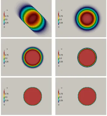
4.1. Test case 1: Pure advection simulation of a circular shape
A circular shape advection test case is proposed in order to evaluate the performance of the LTS scheme in combination with the dimensional
splitting. A square domain [0,330 m]2 discretized on a fine quadrilateral
mesh of 108 900 cells is chosen for this test case, where a circular shape of radius 25 m, centered at (50,50) is set as the initial condition:
u(x, y,0) =
1.0 if p(x−50)2+ (y−50)2 ≤25
0.0 otherwise. (31)
A constant advection velocity of λ = (1,1) and open boundaries are fixed
all over the domain and the numerical results are examined after t=200 s. The conventional upwind scheme (FOU) with a CFL of 0.5 is compared with
the LTS scheme with different CFL numbers in Figure 2. Using even CFL
values, the exact solution is achieved hence odd CFL numbers (1.0, 5.0, 25.0, 75.0 and 151.0) have been chosen in this case. Results highlight that the higher the CFL value chosen, the more accurate the numerical solution is. There are several reasons for this. The main reason is that characteristics are straight lines of constant slope, the temporal error is almost negligible and therefore the spatial accuracy dominates the temporal accuracy. As a consequence, when increasing the CFL number, fewer time steps are done, hence the numerical diffusion associated with the scheme (only first-order accurate) decreases. Apart from that, there is no upper limit to the choice of the CFL number in this case.
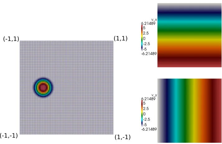
4.2. Test case 2: Advection simulation for a rotating cone
A square 2 m×2 m domain discretized using 8 464 cells (92×92) is used
as a quadrilateral structured mesh to simulate the circular advection of a
(-1,-1)
(1,1) (-1,1)
[image:15.612.117.474.121.352.2](1,-1)
Figure 3: Test case 2: Initial condition and detail of the quadrilateral structured mesh
(left) and velocity field (right) inx-direction(upper) and in y-direction (lower)
u(x, y,0) =
cos2(2πr) r
≤0.25
0.0 otherwise, (32)
where r = p(x+ 0.5)2+y2. The mesh and the initial conditions, as well
as the non-constant velocity field, λ= (−2πy,2πx), are plotted in Figure3.
After one period T (where T=1 in this case), the cone should return to its original position, recovering the initial condition. Also the analytical solution at time T/4, T/2 and 3T/4 can be easily computed.
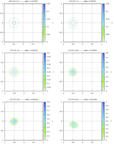
The numerical results computed with the FOU scheme with a CFL of 0.5 and with the LTS scheme with CFL numbers of 1.0, 3.0, 10.0, 20.0 and 60.0
are shown in Figure 4 at T=1. The peak value of each numerical scheme is
also highlighted at the top of each figure.
FOU CFL 0.5 --- uMax = 0.221378
-1 -0.5 0 0.5 1
-1 -0.5 0 0.5 1 0 0.05 0.1 0.15 0.2 0.25 u
LTS CFL 1.0 --- uMax= 0.250347
-1 -0.5 0 0.5 1
-1 -0.5 0 0.5 1 0 0.05 0.1 0.15 0.2 0.25 u
LTS CFL 3.0 --- uMax = 0.452116
-1 -0.5 0 0.5 1
-1 -0.5 0 0.5 1 0 0.05 0.1 0.15 0.2 0.25 0.3 0.35 0.4 0.45 0.5 u
LTS CFL 10.0 --- uMax = 0.750978
-1 -0.5 0 0.5 1
-1 -0.5 0 0.5 1 0 0.1 0.2 0.3 0.4 0.5 0.6 0.7 0.8 u
LTS CFL 20.0 --- uMax = 0.861542
-1 -0.5 0 0.5 1
-1 -0.5 0 0.5 1 0 0.1 0.2 0.3 0.4 0.5 0.6 0.7 0.8 0.9 u
LTS CFL 60.0 --- uMax = 0.912166
-1 -0.5 0 0.5 1
[image:16.612.115.492.149.626.2]-1 -0.5 0 0.5 1 0 0.1 0.2 0.3 0.4 0.5 0.6 0.7 0.8 0.9 1 u
is bigger and fewer steps are required to compute the solution. It is worth
remarking that the numerical results improve on those obtained in [16] where
a sophisticated 2D TVD method is used. On the other hand, the solution is deviating due to the non-uniform velocity field. As fewer time steps are done, the larger magnitude of the time steps means that the dimensional splitting loses too much information about the velocity field to be able to follow com-pletely the correct “pathway”. This deviation is most obvious when using the LTS scheme with a CFL of 60.0, but it is also visible to a lesser extent when the same scheme is applied with with a CFL of 20.0.
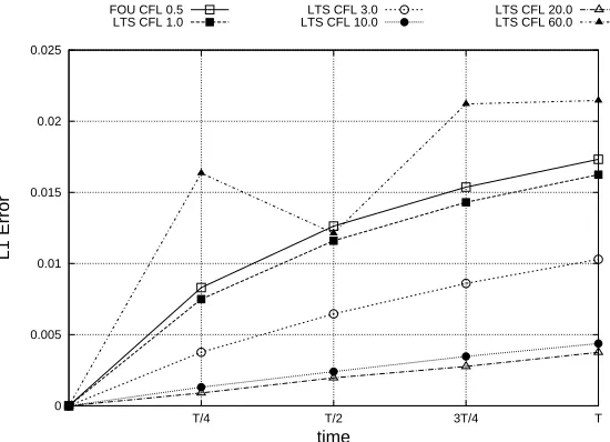
In order to evaluate the quality of the results more fully, the L1 error
between the numerical and the exact solution is also estimated. These errors
are plotted in Figure 5.
0 0.005 0.01 0.015 0.02 0.025
T/4 T/2 3T/4 T
L1 Error
time FOU CFL 0.5
LTS CFL 1.0
LTS CFL 3.0 LTS CFL 10.0
[image:17.612.171.446.312.511.2]LTS CFL 20.0 LTS CFL 60.0
Figure 5: Test case 2: L1errors for the LTS scheme using different CFL numbers.
The LTS scheme with a CFL of 20.0 is the most accurate in terms of this norm, providing the best results. Also, as could be conjectured from
examining Figure 4, the least accurate choice is the LTS with a CFL of 60.0,
even though it achieves the highest peak value. It is not able to reproduce either the exact location or the shape of the rotating cone due to the fact that it is losing important information related to the velocity field when doing these huge time steps.
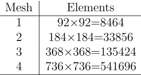
The optimal CFL value is therefore a question of interest. It is not known
starts to decrease. Four different quadrilateral meshes, derived by uniform
mesh refinement (as described by grid refinement 1, Table1), have been used
to clarify which CFL value computes the most accurate solution.
Mesh Elements
1 92×92=8464
2 184×184=33856
3 368×368=135424
[image:18.612.238.376.182.256.2]4 736×736=541696
Table 1: Test case 2. Grid refinement 1. Meshes and elements.
At t=T, the comparison between the numerical solutions computed by the four grids using different CFL values has been carried out. The results
in terms of the L1 norm are shown in Table 2. The symbol ”-” in Table
2 indicates that the results achieved in these cases are the same as for the
previous CFL number.
Mesh CFL L1 Peak value
1 20.0 2.08e-03 0.862
1 30.0 5.12e-03 0.893 1 40.0 1.22e-02 0.924 1 60.0 2.15e-02 0.912 1 100.0 2.51e-02 0.867
1 160.0 -
-2 20.0 1.46e-03 0.937
2 30.0 1.42e-03 0.954
2 40.0 2.99e-03 0.963 2 60.0 4.76e-03 0.971 2 100.0 1.57e-02 0.978 2 160.0 2.51e-02 0.964
Mesh CFL L1 Peak value
3 20.0 6.37e-04 0.968
3 30.0 6.00e-04 0.977
3 40.0 8.40e-04 0.983 3 60.0 1.21e-03 0.988 3 100.0 3.55e-03 0.993 3 160.0 1.23e-02 0.995 4 20.0 3.06e-04 0.984 4 30.0 2.37e-04 0.988
4 40.0 2.23e-04 0.992
4 60.0 4.37e-04 0.994 4 100.0 1.17e-03 0.996 4 160.0 2.92e-03 0.998
Table 2: Test case 2. Grid refinement 1. Comparison between CFL values and error norms on each mesh.
When increasing the number of grid cells, the error in the L1 norm
de-creases, hence ensuring the convergence. Moreover, the peak value increases not only when refining the mesh but also when increasing the CFL value due to the fact that fewer time steps are done, making the scheme less diffusive and allowing higher peak values.
When observing the error in theL1 norm, it is clear that very large CFL
[image:18.612.134.478.370.525.2]exists for which the error is minimal. This optimal CFL number is related not only to the spatial operator (first order) but also to the mesh, being higher when it is refined. For example, for mesh 1, the optimum value is close to 20.0, for mesh 2 and 3, between 20.0 and 30.0 and, for mesh 4, between 30.0 and 40.0. In order to check this hypothesis, an exhaustive grid refinement 2 is proposed.
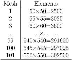
The number of cells of each mesh is summarized in Table3, running each
one with different CFL values from CFL=10.0 to CFL=35.0 (0.5 by 0.5).
Mesh Elements
1 50×50=2500
2 55×55=3025
3 60×60=3600
... ...×...=...
99 540×540=291600
100 545×545=297025
[image:19.612.236.378.255.373.2]101 550×550=302500
Table 3: Test case 2. Grid refinement 2. Meshes and elements.
The considerable amount of data is condensed in Figure6for theL1norm,
where the error and the CFL value for which the norm is at a minimum are plotted against the square root of the number of cells.
When moving towards the right along the x-axis in Figure 6, the number
of cells increases hence the accuracy should be (and is) higher. Moreover, the CFL value for computing the numerical solution with less error (cut-off) grows generally when the mesh increases in number of elements. The more direct implication of this resides in the fact that the CFL value can be increased when refining the mesh. It is worth remarking that the CFL cut-off represents the point at which temporal error is dominating spatial error. Being a first order scheme, the temporal error can become quite high and still not dominate the spatial error. Moreover, in case of having a similar test case with more sharply varying advection speeds, this CFL cut-off would be much lower.
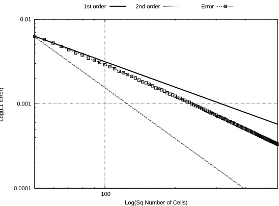
A rate of convergence slightly better than first order is observed in Figure
7where a log-log graph of the error using the optimal values shown in Figure
6and the square root of the number of cells is plotted comparing it with the
0 0.001 0.002 0.003 0.004 0.005 0.006 0.007
50 100 150 200 250 300 350 400 450 500 550 10 12 14 16 18 20 22 24 26 28 30 32 34
L1 Error CFL value
[image:20.612.171.440.146.347.2]Sq Root of Number of Cells Error "Optimum" CFL
Figure 6: Test case 2. Grid refinement 2. MinimumL1error, CFL value for this minimum
error for each mesh
0.0001 0.001 0.01
100
Log(L1 Error)
Log(Sq Number of Cells) 1st order 2nd order Error
[image:20.612.168.442.429.631.2]5. 2D systems of equations: Application to shallow water equations
A 2D hyperbolic non-linear system of equations with source terms can be written in the form:
∂U
∂t +
∂F(U)
∂x +
∂G(U)
∂y =H(U) (33)
or:
∂U
∂t +∇ ·E=H, (34)
in which E=(F,G). Equation (34) is integrated in a volume or grid cell Ω :
∂ ∂t
Z
Ω
UdΩ +
Z
Ω∇ ·
EdΩ =
Z
Ω HdΩ
⇒ ∂t∂
Z
Ω
UdΩ +
I
C
E ·ndC =
Z
Ω
HdΩ, (35)
where n is the outward normal direction, E·n is the normal flux and C
denotes the surface surrounding the volume Ω. The domain is divided into
computational cells, Ωi, using a fixed mesh. Assuming a piecewise constant
representation of the conserved variables [8]
∂ ∂t
Z
Ωi
UdΩ +
NE
X
k=1
(δE)k·nklk =
Z
Ωi
HdΩ, (36)
where nk = (nx, ny) is the outward unit normal vector to cell edge k, δEk=
Ej −Ei, i and j being the indices of the cells sharing the edge k, lk is the
edge length and NE is the number of edges in celli. Following [8], the source
term is linearized as follows
Z
Ωi
HdΩ =
NE
X
k=1
(˜S·n l)nk, (37)
where S is a suitable matrix. Therefore, the fluxes and source terms can
be expressed compactly allowing (36) to be formulated as a homogeneous
∂ ∂t
Z
Ωi
UdΩ +
NE
X
k=1
(δE−S˜)k·nklk= 0. (38)
Applying a local linearization of the problem at each edge, it is possible to
define an approximate Jacobian matrix Jen,k satisfying:
δ(E·n)k =eJn,kδUk. (39)
Using two approximate matrices Pe = (ee1,ee2,ee3), and Pe−1, built using the
eigenvectors of the Jacobian, that diagonalize eJn,k, giving
e
P−k1eJn,kPek =Λek, (40)
where Λek is a diagonal matrix with eigenvalues eλmk in the main diagonal.
According to the local linearisation, the conserved variables as well as the source terms are projected onto the matrix eigenvectors basis:
δUk =PekA˜k (S˜·n)k =PekB˜k (41)
where A˜k = ( ˜α1, α˜2, α˜3)Tk and B˜k = ( ˜β1, β˜2, β˜3)Tk contain the sets of
wave and source strengths, respectively. Therefore, the 2D numerical first order upwind (FOU) scheme can be formulated as follows, dealing with the contributions that arrive to the cell:
Un+1i =Uni −∆t
Ωi NE
X
j=1 3
X
m=1
(˜λ−˜γ˜e)mln
k . (42)
where γm
k is defined as in (15). This update corresponds to (16) for the
one-dimensional shallow water equations and (25) for the two-dimensional scalar
advection equation.
5.1. 2D shallow water equations
The two-dimensional shallow water system of equations can be expressed
as in (33). In particular, U represents the conserved variables
U= (h, qx, qy)T , (43)
whereqx andqy are the unit discharge in thex- andy-direction, respectively,
Fx =
qx,
q2 x
h +
1
2gh
2, qxqy
h T
, Fy =
qy,
qxqy
h , q2 y h + 1 2gh 2 T , (44)
wheregis the acceleration due to gravity. The source terms of the momentum
are due to bed slope and friction
H= (0, gh(S0x−Sf x), gh(S0y−Sf y))T , (45)
where the bed slopes of the bottom level zb are
S0x =−
∂zb
∂x , S0y =− ∂zb
∂y , (46)
and the friction losses are written in terms of Manning’s roughness coefficient
n:
Sf x =
n2u√u2+v2
h4/3 , Sf y =
n2v√u2+v2
h4/3 . (47)
The Jacobian matrix of the normal flux in the 2D model is
J = ∂(E ·n)
∂U =
c2n 0 nx ny
x−uu·n u nx+u·n u ny
c2n
y−vu·n v nx v ny +u·n
, (48)
withn= (nx, ny)T the outward normal vector,u=qx/h,v =qy/h,c=√g h
and u · n = u nx +v ny. In particular, the matrices P and Λ used for
diagonalising this Jacobian matrix and its eigenvalues λm and eigenvectors
em are
P=
1 0 1
u−c nx −cny u+c nx
v−c ny c nx v+c ny
, Λ=
λ1 0 0
0 λ2 0
0 0 λ3
,
e1 =
u−1c nx
v−c ny
, e2 =
−c n0 y
c nx
, e3 =
u+1c nx
v+c ny
,
λ1 =u·n−c , λ2 =u·n, λ3 =u·n+c .
The wave and source strengths derived from the linearization process in
(41) are:
˜
α1 =
δh
2 −
1
2˜c(δq·n−u˜·nδh), α˜2 =
1 ˜
c[δqy −˜v δh)nx−(δqx−u δh˜ )ny)],
˜
α3 =
δh
2 +
1
2˜c(δq·n−˜u·nδh),
˜
β1 =−
1
2c(δz+Sf,n), β˜2 = 0, β˜3 =−β˜1,
˜
uk= √
hiui+
p hjuj √
hi+
p hj
, ˜vk = √
hivi+
p hjvj √
hi+
p hj
, ˜ck =
r
g hi+hj
2 ,
(50)
where ˜u·n = ˜u nx + ˜v ny, δq·n = δqxnx +δqyny and the tilde variables
represent the averaged states at each interface k.
The time step size for the standard first order upwind scheme is governed by the discrete wave celerities defined at each computational cell interface and expressed, in the particular case of a quadrilateral structured grid, as
∆t= CFL min
k,m
Ωi
lk |λ˜mk|
!
, CF L≤0.5. (51)
However, a naive source term discretization could limit the time step size required to ensure numerical stability and positivity of the scheme in complicated test cases. In order to avoid this, a good integration not only of the bed slope source term but also of the friction term, limiting the amount of the numerical source instead of reducing the time step size, is assumed.
More details relating to this procedure can be found in [8, 9].
Once the correct formulation of the source term discretization has been
adopted, the restriction in (51) can be relaxed when using the 2D LTS scheme
and the dimensional splitting technique. Once the time step size is calculated, the procedure consists of computing the contributions at each interface and
sending them along the x- or y-direction with their corresponding time step
size according to (29).
The information is sent from each computational cell interface in a similar
way to the 1D case, replacing ∆xby Ωi/lk in the case of quadrilateral
k sharing the cells i and j, the interface can be relabelled as i+ 1/2 (based
on the evolution operator πx) and cell j as i+ 1, simplifying the notation
when referring to the previous or subsequent neighbouring cells. With this notation:
Ifλem
i+1/2 >0
(˜γ ee)mi+1/2 is subtracted from cellsi+ 1,· · · , i+µm i+1/2
(ν−µ)m
i+1/2(˜γ ee) m
i+1/2 is subtracted from celli+µmi+1/2+ 1
(52)
Ifλem
i+1/2 <0
(˜γ ee)mi+1/2 is subtracted from cellsi,· · · , i+µm
i+1/2+ 1
(ν−µ)m
i+1/2(˜γ ee) m
i+1/2 is subtracted from celli+µmi+1/2
(53)
where m = 1,2,3, ˜γkm = α˜− β˜
˜
λ !m
k
, νkm = ∆t lk Ωi
e
λmk and µm
k =int(νkm).
Af-ter each sub-iAf-teration inside the whole time step, the cells have to be updated also considering the information from the boundaries. The procedure for one time step is the same as that presented in Section 3.2, sending the information
according to (52) and (53).
5.1.1. Wet/dry fronts and CFL limit
The formulation for a wet/dry front is an issue of importance in the 2D shallow water model in order to prevent instabilities and to prevent negative values of water depth. As the dimensional splitting technique divides each time step into three sub steps solving three 1D problems, the way of dealing
with wet/dry interfaces is explained for the 1D system (9).
The treatment of wet/dry fronts in the LTS scheme is previously
men-tioned in [6] where a reduction in the time step size is enforced to recover
the conventional upwind scheme when a wet/dry front appears. In order to avoid reducing the time step size in these kinds of situations, a short
proce-dure consisting of two steps is proposed in this work, following [8]. The first
✲ ✻
❅ ❅ ❅ ❅
h
n iU
nih
ni+1
= 0
U
ni+1h
∗∗i+1
h
∗i
e
λ
2e
λ
1x
t
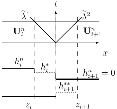
[image:26.612.216.408.126.306.2]z
iz
i+1Figure 8: Sketch of the intermediate states in the (x, t) plane for the subcritical case.
Wet/dry interfaces and negative value in the intermediate stateh∗∗
i+1.
front is located between cells i and i+ 1. The requirement of the positivity
of the intermediate states derived from the Riemann Problem (see Figure
8) between cells i and i+ 1 allows determination of the wet/dry interfaces.
They are expressed as follows:
U∗i =Uni + (˜γee)1i+1/2
U∗∗i+1 =Uni+1−(˜γee)2i+1/2
(54)
where ˜γ and ee are defined in Section 2. More detailed explanation can be
found in [8]. In fact, the following rule is adopted:
• If hn
i+1 = 0 and h∗∗i+1 <0 set i+ 1/2 as a solid interface.
• If hn
i = 0 and h∗i <0 set i+ 1/2 as a solid interface.
where h∗∗
i+1 and h∗i are defined in (54).
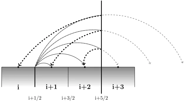
Once all the contributions are calculated and the wet/dry solid interfaces are identified, the second step is applied: the information from each compu-tational interface is sent depending on the character (solid or not solid) of
the involved interfaces. For example, consider νi+1/2 = 4.3 and the interface
to cell i+ 1 and to cell i+ 2. However, asi+ 5/2 is detected as a solid in-terface, information cannot pass through this “wall” and hence is sent back
to the corresponding cells as in the reflection technique [6]. It is illustrated
in Figure 9.
i i+1 i+2 i+3
[image:27.612.151.468.197.371.2]i+1/2 i+3/2 i+5/2
Figure 9: Example of the procedure to send the information with a wet/dry solid interface .
This procedure reduces the appearance of negative water depth values. However, the labelling of the wet/dry interfaces as solid or not comes from a local analysis, but the information is sent far from the neighbouring cells. Therefore, the problem of negative values for the water depth is not totally eliminated. In these extreme cases, an option is to reduce the time step to half the size and to recompute.
On the other hand, a parameter ξ was introduced in [6] to internally
reduce the initial target CFL value in the presence of sharp discontinuities or large source terms. The LTS proposed may produce wrong results in the presence of strong discontinuities in the solution behaving as shocks. To avoid that, at the beginning of every time step the relative size of the discontinuities is evaluated and the target CFL is adjusted accordingly. Then, it is used globally as in any other time step so that the calculations run always with a global time step that is controlled by the most restrictive cell.
The new wet/dry strategy requires a revision of the mentioned parameter in order to avoid undesirable reductions in the target CFL value. In fact,
ξ1 =
mini{hi, hi+1,|δhi+1/2|} |δhi+1/2|
, ξ2 =
mini{|di|,|di+1|,|δdi+1/2|} |δdi+1/2|
, (55)
for 1 ≤ i ≤ N, where h is the water depth, d = h+z is the water surface
level and 0 ≤ ξ ≤ 1. This parameter ξ gives a measure of the size of the
discontinuity, being closer to 0.0 when the discontinuity is strong and around
1.0 when the variables h and d are smooth or gradually varying.
However, the evaluation of ξ in (55) when hi or hi+1 is zero enforces the
recovery of the FOU scheme. Therefore, wet/dry fronts must be reformulated
inside (55) in order to refrain from reducing the CFL initially chosen and a
tolerance (T OL) for the variables is proposed. For example, parameter ξ1
will only act if
min{hi, hi+1,|δhi+1/2|}> T OL , (56)
with an analogous condition imposed for parameter ξ2, replacing h by d. In
this work, T OL= 0.05 m.
6. Numerical results for the 2D shallow water equations
In this section, four challenging time-dependent test cases are presented to test the performance of the 2D LTS scheme and to introduce the wet/dry treatment explored in this work. The CPU time is evaluated.
6.1. Test case 3: Circular dam break
Dam break problems are widely used to test the behaviour of a numerical
scheme. Consider a square frictionless domain Ω = [0,200 m]2 discretized in
a quadrilateral regular mesh of 40 000 cells (200×200) with flat bed elevation
and closed boundaries. The initial condition consists of still water of depth 1 m over all the domain except a circular sector in the lower left corner which
has a 4 m depth of water (see Figure 10):
h(x, y,0) =
4.0 ifpx2+y2 ≤100m
1.0 otherwise. (57)
The boundary treatment was previously considered in [6] for the 1D
Figure 10: Test case 3: Initial state and sampling line.
closed boundaries, the reflection technique, that considers the corresponding downstream edge as a mirror and reflects the waves, is utilised in this work. The numerical results achieved by the conventional FOU scheme with a CFL of 1.0 are compared with those obtained by the LTS scheme with CFLs of
2.0, 4.0 and 8.0 at t = 12 s and t= 20 s (Figures 11 and 12 respectively) for
the water depth.
Although spurious oscillations are detected near the location of the shock when increasing the CFL number, the solutions seem to be less diffusive, not only in the shock front but also near the rarefaction. In order to
corrobo-rate this hypothesis, the comparison through the line plotted in Figure 10is
considered, where a high resolution numerical solution (from now on called ’exact’) can be computed evaluating the problem as a 1D problem on the
radial direction. Figures 13and 14show the exact and numerical results at
t = 12 s for the water depth and for the x- and y-unitary discharge
respec-tively. The LTS scheme becomes visibly less diffusive as the CFL number is increased, although several oscillations appear. However, the velocity field tends to be more sensitive and larger oscillations near the shock fronts are
clearly visible in Figure 14.
6.2. Test case 4: Dam break over adverse slope
1 1.5 2 2.5 3 3.5 4
0 50 100 150 200 250 300
water depth (m)
longitudinal coordinate (m)
[image:32.612.133.481.134.378.2]FOU CFL 0.5 LTS CFL 2.0 LTS CFL 4.0 LTS CFL 8.0 exact
Figure 13: Test case 3: Exact and numerical results for water depth att= 12 s.
discontinuity is over a dry bed, the test case contains all the elements that represent a challenge in shallow flow modelling. A test case, consisting of a dam break over dry bed with adverse slope, is performed as a good measure of the behaviour of the wet/dry front treatment in unsteady flow. Consider the same domain and discretization as the previous test case. The friction is
modelled now using a Manning friction coefficientn = 0.03 s/m13. The initial
condition and the bed level (see Figure 15) are set to
h(x, y,0) =
2.0 if px2+y2 <100
0.0 if 100<px2+y2 <√2 100.0
0.0 if x >√2 100.0,
(58)
z(x, y) =
0.0 if px2 +y2<100
0.0 if 100<px2+y2 <√2 100.0
p
2(x2+y2)
100 −2 if x >
√
2 100.0.
(59)
0 1 2 3 4 5
0 50 100 150 200 250 300
x-unitary discharge (m/s)
longitudinal coordinate (m) FOU CFL 0.5
LTS CFL 2.0 LTS CFL 4.0 LTS CFL 8.0 exact
0 1 2 3 4 5
0 50 100 150 200 250 300
y-unitary discharge (m/s)
longitudinal coordinate (m) FOU CFL 0.5
[image:33.612.119.501.181.309.2]LTS CFL 2.0 LTS CFL 4.0 LTS CFL 8.0 exact
Figure 14: Test case 3: Exact and numerical results at t = 12 s for x-unitary discharge
(left) andy-unitary discharge (right).
[image:33.612.115.494.402.601.2]0 0.5 1 1.5 2
0 50 100 150 200 250 300
water level surface (m)
longitudinal coordinate (m) Bed level FOU CFL 0.5 LTS CFL 3.7
0 0.2 0.4 0.6 0.8 1 1.2 1.4 1.6 1.8 2
0 50 100 150 200 250 300
water level surface (m)
longitudinal coordinate (m) Bed level
FOU CFL 0.5 LTS CFL 3.7
0 0.2 0.4 0.6 0.8 1 1.2 1.4 1.6 1.8 2
0 50 100 150 200 250 300
water level surface (m)
longitudinal coordinate (m) Bed level
FOU CFL 0.5 LTS CFL 3.7
0 0.2 0.4 0.6 0.8 1 1.2 1.4 1.6 1.8 2
0 50 100 150 200 250 300
water level surface (m)
longitudinal coordinate (m) Bed level
[image:34.612.119.499.137.408.2]FOU CFL 0.5 LTS CFL 3.7
Figure 16: Test case 4. Longitudinal profile along the diagonal line achieved by the FOU
scheme and the LTS scheme with a CFL of 3.7 at t= 10 s (upper left), att= 50 s (upper
right), at t= 100 s (lower left) and att= 40 000 s (lower right)
previous test case) is plotted in Figure 16at t = 10 s, t= 50 s and t = 100 s
comparing the numerical results achieved by the FOU scheme and the LTS scheme with an arbitrarily chosen CFL value of 3.7. Also the final state
at t = 40 000 s is shown in Figure 16 (lower right). The same source term
treatment, checking the non-negativity property of the intermediate states of the Riemann Problems, has been implemented in both simulations.
6.3. Test case 5: tsunami test case
The simulation of a tsunami event modelled in a 1/400 laboratory scale
[18, 19] is used to demonstrate the applicability of the LTS scheme to
un-steady real problems. Gauging points were located at
P1 = (4.52,2.196), P2 = (4.52,1.696), P3 = (4.52,1.196), (60)
where the evolution in time of the water level surface is registered. Figure
17 shows the bathymetry of the reduced model as well as the location of
the gauging points mentioned. According to the reported bed material, the
friction is modelled with a Manning coefficient ofn = 0.01 s/m13. More details
[image:35.612.126.480.328.478.2]about the description and the experimental data can be found in [19, 20].
Figure 17: Test case 5: Bed elevation and probe locations.
The initial condition is fixed as a constant water surface level ofh+z = 0.0
and the domain ([0,5.488] × [0,3.388]) has been discretized with a mesh
of 23 716 cells (196 × 121). The boundary conditions are considered as
closed vertical sidewalls (as in the laboratory model) except the incident wave coming from offshore, defined as a variation in time of the water depth (see
Figure19). It is worth remarking that, in this finite volume implementation,
the information given as the boundary condition is imposed at the center of the boundary cells.
The numerical simulation has been carried out using the FOU scheme with a CFL of 0.5 and the LTS scheme with three different CFL values: 2.4,
Figure 18: Test case 5: 3D plot of the water level surface att= 13 s (upper) andt= 18 s (lower)
t = 18 s are illustrated in Figure 18, simulated with the LTS scheme with
a CFL of 4.8. At t = 13 s the shoreline is moving backward due to the
depression wave, but byt = 18 s the wave has reached the end of the domain
and has been reflected.
The time evolution registered experimentally at measured points P1, P2 and P3 is also compared with the numerical results obtained by the FOU
scheme and the LTS scheme with the mentioned CFL values in Figure 19.
-0.015 -0.01 -0.005 0 0.005 0.01 0.015 0.02
0 5 10 15 20
h+z (m) time (s) -0.02 -0.01 0 0.01 0.02 0.03 0.04 0.05
0 5 10 15 20 25
h+z (m)
time (s) P1 experimental
P1 FOU P1 LTS CFL 2.4 P1 LTS CFL 4.8 P1 LTS CFL 7.2
-0.02 -0.01 0 0.01 0.02 0.03 0.04 0.05
0 5 10 15 20 25
h+z (m)
time (s) P2 experimental
P2 FOU P1 LTS CFL 2.4 P1 LTS CFL 4.8 P1 LTS CFL 7.2
-0.02 -0.01 0 0.01 0.02 0.03 0.04 0.05
0 5 10 15 20 25
h+z (m)
time (s) P3 experimental
[image:37.612.118.500.246.523.2]P3 FOU P1 LTS CFL 2.4 P1 LTS CFL 4.8 P1 LTS CFL 7.2
0 0.001 0.002 0.003 0.004 0.005
0 5 10 15 20 25
L1
error
time (s) P1 FOU
P1 LTS CFL 2.4 P1 LTS CFL 4.8 P1 LTS CFL 7.2
0 0.0005 0.001 0.0015 0.002 0.0025
0 5 10 15 20 25
L1
error
time (s) P2 FOU P2 LTS CFL 2.4 P2 LTS CFL 4.8 P2 LTS CFL 7.2
0 0.0005 0.001 0.0015 0.002 0.0025
0 5 10 15 20 25
L1
error
[image:38.612.118.500.138.397.2]time (s) P3 FOU P3 LTS CFL 2.4 P3 LTS CFL 4.8 P3 LTS CFL 7.2
Figure 20: Test case 5: L1-error at probes P1, P2, and P3 relative to a grid converged
solution
to the experimental measurements. Also the results achieved by the three different CFL values used for the LTS scheme do not generate ’a priori’ many differences. It is due to the internal reduction in the time step size during the computation to avoid negative water depth values.
In order to strengthen this hypothesis, the time evolutionL1-error in these
probes P1, P2, and P3 relative to a grid converged solution (the maximum
available resolution data, 392 × 242 cells) is plotted in Figure20. Firstly, as
probes are placed in a critical location, just behind the island, with wet/dry
transitions, the L1-error can provide a very local estimation of the error
Figure 21: Test case 6: Topography and location of the boundaries
6.4. Test case 6: Real world configuration: Ebro river
The proposed LTS scheme is now applied to a realistic test case in order to evaluate its uncertainty in the flooding prediction. For this purpose, a me-andering reach of the Ebro river (Spain) is used. The Digital Terrain Model (DTM) including the bathymetry was provided by the Ebro River Basin
Ad-ministration (www.chebro.es). The domain (3×2km2) is discretized in 300
× 200 square cells, integrating the information coming from the DTM. This
grid will be used for the simulation of a flooding event with the LTS scheme with CFL 4.2 and with the FOU scheme with CFL 0.5. A steady state of 100
m3/s is computed and set as the initial condition before the flooding event,
which represents the failure of a dam located upstream. Therefore, the inlet boundary condition consists of a one day abrupt hydrograph raising to 1400
m3/s in 180 s and decreasing afterwards linearly during the rest of the day
(see Figure 22, left). With this choice, all kind of scenarios such as sharp
shocks, wetting and drying situations, are present. A free flow condition is chosen as the outlet boundary. The location of the inlet and outlet bound-ary conditions, as well as the topography of the test case are displayed in
Figure 21. According to the aerial photograph of the domain, a Manning’s
roughness map is considered, shown in Figure 22(right).
0 200 400 600 800 1000 1200 1400 1600
0 5 10 15 20
discharge (m
3/s)
[image:40.612.125.490.127.229.2]time (h) Inlet Hydrograph
Figure 22: Test case 6: Inlet hydrograph and Manning’s roughness map
grid of 1500000 (1500 × 1000) squared cells using the first order upwind
scheme with CFL 0.5 is chosen as a reference solution in order to compare the schemes mentioned above. The comparison is firstly done using map errors. Therefore, a mapping from the coarse to the fine grid is performed to be able to extract the spatial distribution of the error. The relative error with
respect to the reference solution is analysed for the variables h and velocity
magnitude (modU). As an example, a map error is included corresponding to
t=3h (Figure 23) for the FOU scheme (left) and for the LTS scheme (right).
The meaning is as follows: 0.0 means no differences, 1.0 has to be understood as the scheme (FOU or LTS) is wetting a cell that is completely dry on the reference solution and -1.0 is a dry zone for the scheme (FOU or LTS) that is wetted on the reference solution.
As can be seen, the error for both schemes is almost totally located at the floodplain, where the coarse grid is overestimating the flooding area, possibly due to the incorrect definition of levees. It can be concluded that in terms of water depth, at t=3h, the LTS scheme computes a more accurate solution than the FOU scheme. The main factor responsible for this is the wet/dry treatment, which seems to be more restrictive in this situation. The velocity magnitude is overall well-reproduced in the main river, while the flooding extension overestimates it in the floodplain.
In order to have a quantitative measure of the error, Figure 24 shows
two graphs. On the left, the evolution of the L1-error along the domain over
the 24h hydrograph is extracted for the water depth and for the velocity magnitude. On the right, the evolution of the flooded area computed by each model is compared against the flooded area achieved by the reference solution.
Figure 23: Test case 6: Map error of water depth for the FOU scheme (upper left) and for the LTS scheme (upper right) at t=3h. Map error of velocity magnitude for the FOU scheme (lower left) and for the LTS scheme (lower right) at t=3h.
0 0.1 0.2 0.3 0.4 0.5 0.6
0 5 10 15 20
L1
error
time (h) h L1-error FOU
h L1-error LTS
modU L1-error FOU modU L1-error LTS
500000 1e+06 1.5e+06 2e+06 2.5e+06 3e+06 3.5e+06 4e+06 4.5e+06
0 5 10 15 20
flooded area (m
2)
time (h)
Reference FOU LTS
Figure 24: Test case 6: Evolution of the L1-error (left) and flooded area (right) with
[image:41.612.116.496.482.616.2]obtained by the reference solution although both models overestimate the flooded area.
6.5. Computational time
The use of a LTS scheme with larger CFL values than the conventional
schemes should imply a reduction in the computational burden. Table 4
summarizes the CPU time consumed by each scheme (FOU and LTS) in each test case of relevance. Note that the CFL value of 0.5 (the maximum allowable in squared meshes) is used for the computation with the FOU scheme and the number of cells in both models is always the same for each test case.
Test case FOU time (s) LTS Speed-up
CFL number time (s)
4 11227 CFL 3.7 5105 2.199
5 72 CFL 2.4 48 1.5
CFL 4.8 40 1.8
CFL 7.2 46 1.565
[image:42.612.138.473.294.454.2]6 22380 CFL 4.2 7405 3.022
Table 4: CPU time consumed by the each model in each test case of relevance
7. Conclusions
The implementation of a 2D Large Time Step (LTS) finite volume method has been presented in this work. The extension to two-dimensional domains is achieved by means of the dimensional splitting technique. Previous advances related to the source term discretization and boundary conditions treatment detailed for the 1D case are preserved due to the splitting procedure, solving “by rows” or “by columns” three 1D problems per time step.
The LTS scheme has been presented for the 2D scalar case, dealing with constant and variable velocity fields and with boundary conditions. An easy to follow algorithm is detailed. Some considerations have been highlighted connected to the boundary treatment and information provided by the char-acteristic curves has been utilised. The scheme is less diffusive than the first order upwind (FOU) scheme with a CFL of 0.5 for the 2D scalar equation.
The extension to systems of equations has been described generally, and is then applied to the 2D shallow water equations with source terms. Wet/dry fronts are of interest in any 2D shallow water model. A short procedure based on the reflection technique at closed boundaries is proposed here for dealing with them. It consists of identifying the wet/dry solid interfaces and ensur-ing that information is not sent through them. Associated with the wet/dry treatment, the CFL limit, that reduces the time step size in the presence of
large discontinuities has been reformulated according to [8]. The proposed
wet/dry treatment, combined with a careful source term discretization, en-sures the well-balanced property and makes the reduction in the time step size and the appearance of negative values of the water depth less extreme.
Realistic and notably complex test cases have been suggested to evalu-ate the performance of the 2D LTS scheme under exacting conditions. As expected, it is demonstrated to be less diffusive the standard FOU scheme, although several oscillations appear in the most extreme situations, as in the 1D case. Moreover, the wet/dry fronts are well reproduced, achieving results which are as good as those of the conventional first order upwind scheme, but with the larger CFLs giving the potential for faster computation.
References
[1] Z. Qian and C-H. Lee, A class of large time step Godunov schemes for hyperbolic conservation laws and applications, J. Comput. Phys., 230 (2011) 7418–7440.
[2] M. R. Norman, R. D. Nair and F.H.M. Semazzi, A low communica-tion and large time step explicit finite-volume solver for non-hydrostatic atmospheric dynamics, J. Comput. Phys., 230 (2011) 1567–1584.
[3] Z. Qian and C-H. Lee, On large time step TVD scheme for hyperbolic conservation laws and its efficiency evaluation, J. Comput. Phys., 231 (2012) 7415–7430.
[4] R.J. Leveque, Large Time Step Shock-Capturing Techniques for Scalar Conservation Laws, SIAM J. Numer. Anal., 19, No. 6 (1982), 1091–1109
[5] R.J. Leveque, A Large Time Step Generalization of Godunov’s Method for System of Conservation Laws, SIAM J. Numer. Anal., 22 (1985) 1051–1073.
[6] M. Morales-Hern´andez, P. Garc´ıa-Navarro and J. Murillo, A large time
step 1D upwind explicit scheme (CFL>1): application to shallow water
equations, J. Comput. Phys., 231 (2012) 6532–6557
[7] J. Murillo, J. Burguete, P. Brufau and P. Garc´ıa-Navarro, The influ-ence of source terms on stability, accuracy and conservation in two-dimensional shallow flow simulation using triangular finite volumes, Int. J. Numer. Meth. Fluids, 54 (2007) 543–590.
[8] J. Murillo and P. Garc´ıa-Navarro, Weak solutions for partial differential equations with source terms: Application to the shallow water equations, J. Comput. Phys., 229 (2010) 4327–4368.
[9] J. Murillo and P. Garc´ıa-Navarro, Wave Riemann description of friction terms in unsteady shallow flows: Application to water and mud/debris floods, J. Comput. Phys., 231 (2012) 1963–2001.
[10] J. Murillo, P. Garc´ıa-Navarro, P. Brufau, and J. Burguete, Extension
of an explicit finite volume method to large time steps (CFL>1):
[11] P.L. Roe, Approximate Riemann solvers, parameter vectors and differ-ence schemes, J. Comput. Phys., 43 (1981) 357–372.
[12] M.E. V´azquez-Cend´on, Improved treatment of source terms in upwind schemes for the shallow water equations in channels with irregular ge-ometry. J. Comput. Phys. 148, (1994), 497–498.
[13] E.F. Toro.Riemann solvers and numerical methods for fluid dynamics.
Springer, Berlin, pp. 526, 1997.
[14] J. Murillo, B. Latorre, P. Garc´ıa-Navarro, A Riemann solver for un-steady computation of 2D shallow flows with variable density, J. Com-put. Phys., 231 (2012) 4775–4807,
[15] G. Strang, On the construction and comparison of different schemes. SIAM J. Numer. Anal., 5 (1968) 506–517.
[16] J. Hou, F. Simons and R. Hinkelmann, A new TVD method for advec-tion simulaadvec-tion on 2D unstructured grids, Int. J. Numer. Meth. Fluids, 71 (2012) 1260–1281.
[17] A. Harten, On a large time-step high resolution scheme, Math. Comput., 46(174) (1986) 379-399.
[18] Matsuyama M, The Third International Workshop on Long-wave Runup Models. Wrigley Marine Science Center: Catalina Island, CA, 2004.
[19] Liu, P.L.-F., H. Yeh, and C. Synolakis : Advanced Numerical Models for Simulating Tsunami Waves and Runup. Advances in Coastal and Ocean
Engineering, 10, (2008) pp. 250. Available at 1 (accessed 28th October
2013)
[20] J. Burguete, P. Garc´ıa-Navarro and J. Murillo, Friction term discretiza-tion and limitadiscretiza-tion to preserve stability and conservadiscretiza-tion in the 1D shallow-water model: application to unsteady irrigation and river flow, Int. J. Numer. Meth. Fluids, 58 (2008) 403–425.