Efficient real time path integrals for non Markovian spin boson models

PAPER

Ef

fi

cient real-time path integrals for non-Markovian spin-boson

models

A Strathearn, B W Lovett and P Kirton

SUPA, School of Physics and Astronomy, University of St Andrews, St Andrews, KY16 9SS, United Kingdom

E-mail:[email protected]

Keywords:non-Markovian, path integral, spin-boson model

Abstract

Strong coupling between a system and its environment leads to the emergence of non-Markovian

dynamics, which cannot be described by a time-local master equation. One way to capture such

dynamics is to use numerical real-time path integrals, where assuming a

finite bath memory time

enables manageable simulation scaling. However, by comparing to the exactly soluble independent

boson model, we show that the presence of transient negative decay rates in the exact dynamics can

result in simulations with unphysical exponential growth of density matrix elements when the

finite

memory approximation is used. We therefore reformulate this approximation in such a way that the

exact dynamics are reproduced identically and then apply our new method to the spin-boson model

with superohmic environmental coupling, commonly used to model phonon environments, but

which cannot be solved exactly. Our new method allows us to easily access parameter regimes where

we

find revivals in population dynamics which are due to non-Markovian backflow of information

from the bath to the system.

1. Introduction

Finding accurate descriptions of open quantum systems strongly coupled to external environments is essential for understanding how quantum systems lose their coherence[1,2]. For example, the behaviour of quantum dots in semiconductors[3–7]and NV centres in diamonds[8,9]can both require a strong coupling description. Strong coupling inevitably leads to the emergence of non-Markovian phenomena in such systems, and this has been experimentally demonstrated[10], opening up the potential for exploiting non-Markovianity as a resource in developing quantum technologies[11,12].

In this paper we will introduce a new way of modelling a strongly coupled environment, developing previous approaches based on Feynman’s path integral formulation of open quantum systems[13–16]. In particular, we will show how a technique based on discretisation of the Feynman influence functional—the so-called

augmented density tensor(ADT)can be modified to significantly improve the convergence of simulations in its numerical implementation. This allows us to study the spin-boson model in a very strong coupling regime that shows clear non-Markovian behaviour that we quantify with the widely-used trace distance measure[17].

When the system-environment coupling is weak, Born–Markov master equations[2,18]provide a perturbative approach in which the environment is assumed to be Markovian i.e. memoryless. While this approach is very successful within its range of applicability[2,19], for many physical applications the(rather severe)approximations made when deriving these types of master equation are not justified. A common approach to go beyond the weak coupling regime is to use a polaron-transformed master equation[19–24]. Such an approach has been used to understand features which could not be explained in weak coupling for

semiconducting quantum dots[20], circuit QED[25], energy transfer in biological systems[22,26,27]and Bose–Einstein condensation of photons in optical microcavities[28,29]. However, a polaron master equation comes at the expense of introducing a restriction on the renormalized system Hamiltonian terms. Other master equation based techniques such as Nakajima–Zwanzig projection operator equations[2], time-convolutionless OPEN ACCESS

RECEIVED

19 April 2017

REVISED

20 July 2017

ACCEPTED FOR PUBLICATION

21 August 2017

PUBLISHED

14 September 2017

Original content from this work may be used under the terms of theCreative Commons Attribution 3.0 licence.

Any further distribution of this work must maintain attribution to the author(s)and the title of the work, journal citation and DOI.

master equations[2], reaction co-ordinate methods[30]and Keldysh–Lindbald equations[31]are able to pertubatively go beyond both the Born and Markov approximations but are still, in practice, limited to restricted parameter regimes.

One can overcome this restriction by using non-perturbative approaches. One class of such methods uses the Feynman path integral representation and formally integrates out the environmental degrees of freedom. Then all effects of the system-environment coupling are described by an influence functional[13]that acts only on the reduced system trajectories. This representation of an open quantum system has proved useful in developing both analytical and numerical methods. As an example, the non-interacting blip approximation[15] is a successful non-perturbative analytical method for understanding the spin-boson model, derived from the influence functional. However, this is only applicable for a relatively small range of parameters.

A versatile numerical method forfinding the dynamics of these kinds of systems is the ADT scheme,first introduced as the quasi-adiabatic propagator path integral by Makri and Makarov[32,33]. This is, in principle, applicable to environments with arbitrary spectral density. The main drawback to this technique is the

exponential scaling of storage requirements with system size, though in some cases ways of reducing these requirements are known[34,35]. Hence, the primary use of this method is to calculate the of dynamics of few-level systems in contact with a bosonic reservoir. The ADT has been used to calculate equilibrium correlation functions[36]and system steady states[32]. In addition, multiple spatially separated sites coupled to the same bath can be accounted for[37], and additional Markovian dynamics in the reduced system can be incorporated at no additional computational cost[38]. Practically, the ADT method has been put to use effectively in, for example, benchmarking master equation methods[39,40], simulating systems in the difficult-to-access regime of subohmic system-bath coupling[41]and investigating dissipative dynamics of charge qubits in realistic environments[42,43]. Very recently, it was shown that, as long as the operator which couples to the environment only acts in a small section of Hilbert space much larger systems can be treated at only small numerical cost[44].

Other numerical approaches are able to accurately describe non-perturbative dynamics in spin-boson systems. The hierarchical equations of motion method[45]is regularly used to benchmark master equation approaches[30]. Techniques based on the numerical renormalisation group have been successfully applied to quantum impurity dynamics by mapping baths characterised by particular spectral density forms into semi-infinite one-dimensional chains[46–49]. Ansatz wavefunctions such as matrix product states[50]can also be used following a similar mapping[51], while approaches based on a Monte Carlo sampling of the path integral can be used to look at dynamics[52,53]. For a recent review of many of the techniques mentioned above see Vega and Alonso[54].

The key approximation made in the ADT scheme is that the bath is assumed to have a sharply definedfinite memory time, and so non-Markovian effects are givenfinite range. This is intuitively justified since, for infinite bosonic baths, all correlations decay to negligible size infinite time. The performance of this method has been successfully tested against other numerical methods[55]and exact analytics[56]. However, the full

consequences of the sharp memory time cutoff and how this affects convergence have not been addressed. Moreover, it has been recognised that for superohmic environments using this approximation results in both quantitatively and qualitatively incorrect asymptotic long time behaviour[57,58]. In this paper we will show that, in certain cases, throwing away small long time correlations beyond the cutoff can have dramatic effects, including unbounded growth of density matrix elements. We then propose a less severe way to make this approximation which does not suffer from the same problems.

The structure of this paper is as follows: in section2we introduce the ADT scheme in detail. Following this, in section3, we investigate the results of enforcing thefinite memory approximation upon the exact solution of a pure dephasing model and identify the class of bath spectral densities for which thefinite memory

approximation has most drastic effects. We then propose an alternative way of taking thefinite memory approximation such that the exact solution of the dephasing model is reproduced at all times for arbitrary spectral densities. In section4we go on to apply our method to the spin-boson model with a highly non-Markovian superohmic bath. Wefind that our modified memory cutoff significantly improves convergence in this model and allows us to observe revivals in the population dynamics due to excitation exchange with the environment. We also calculate the trace distance measure of non-Markovianity in this model,finding regimes of non-Markovian behaviour that we compare to the population revivals. Finally, in section5we summarise our results.

2. ADT scheme

are those consisting of a small system of interest linearly coupled to a macroscopic bath of bosonic modes. The generic Hamiltonian of such models is

å

å

= + +

a a

a

a a a

ˆ ˆ † ( )

H H0 s B a a 1

=H0+HB, ( )2

whereH0is the free system Hamiltonian andHBcontains both the free bath Hamiltonian and the system-bath

interaction. Here,aa†(aα)andwaare the creation(annihilation)operators and frequencies of theαth oscillator. The system operatorsˆcouples to the bath operatorsBˆa=g aa a+g aa a* †with coupling constantsgα.

To simplify our notation we work in the Liouvillian representation such that operators in Hilbert space are represented by vectors in Liouville space. To parameterise theDdimensional Hilbert space of the system we use theDeigenstates ofsˆ. Operators in this space are vectorized in the following way

å

å

r = r +ñá - º r ññ º r ññ

+ +

-ˆ_R ∣s s ∣ ∣S ∣ , ( )3

s s s s

S

S R

,

where the sum overSruns over theD2pairs of{s+,s-}ands sˆ∣+ñ = s s+ +∣ ñand likewise fors-. We use the notation∣xññto mean a vector in Liouville space. The bath Hilbert space can also be represented in a similar way, though we do not need to define its basis explicitly in what follows. The evolution of the reduced system, assuming factorising initial conditions is now represented as:



r ññ = r ññr ññ

∣ _R( )t Tr e[ t∣ ( ) ∣0 ], ( )4

R

B B

with the Liouvillian=₀+_B, where0andBgenerate coherent evolution caused byH0andHB

respectively. Recently it has been shown[38]that additional Markovian non-unitary dynamics of the reduced system can be incorporated by adding Lindblad-type dissipators into the free system Louivillian0, making it

straightforward to account for coupling to other baths for which the Born–Markov approximations are well justified. In addition to factorising initial conditions we also assume the initial state of the bath is that of thermal equilibrium when no system is presentrB=exp(-åa a a aw a a† T) , with temperatureTand partition

function.

Thefirst approximation made to make equation(4)computable is to factorise the long time propagator intoN short time propagatorset =(eDt N) _{and then to employ a Trotter splitting between the system and bath parts[59]}

D _» D D _{( )}

e t e B te 0 t, 5

on each of these. The error introduced in this process is(Dt2)_{. We note that the argument that now follows can} be easily adapted to use a symmetrized Trotter splitting[32,33,60]that improves the error to(Dt3)_{. All the} numerical results we present do include this symmetrized splitting, but for simplicity of notation we will use the definition in equation(5)here.

Tracing out the bath degrees of freedom then results in a reduced density matrix at timetN=N tD , whose

elements are

å

r = r

¼

-∣ ( ) ({ }) ({ }) ∣ ( ) ( )

S_{N R N}t F S I S S 0 6

S S

k k 0 R

N

0 1

The functionsF({ })Sk andI({ })Sk constitute the free part of the evolution and the discretized Feynman

influence functional respectively, and are given by





= áá ññ

=

D

-({ }) ∣ ∣ ( )

F Sk S e S 7

j N

j t j

1

1

0



= á ñá ñ

=

+ - D -+

-- D

-∣ ∣ ∣ ∣ ( )

s e s s e s , 8

j N

j H t j j H t j

1

i

1 1 i

0 0

*

å å

= - - -= ¢-= + -- ¢ ¢+ - ¢ ¢ -⎛ ⎝ ⎜ ⎞ ⎠ ⎟ ({ }) ( )( ) ( )

I Sk exp s s s s . 9

k N

k k

k k k k k k k k

1 1

The coefficientsh_{k k- ¢}quantify the non-Markovian‘interaction’between the reduced system at different timestk

andtk¢and are defined as

ò ò

ò ò

h =

¢ -   ¢ ¹ ¢

¢ -   ¢ = ¢ - ¢ - ¢-_¢ ¢ - -⎧ ⎨ ⎪⎪ ⎩ ⎪ ⎪ ( ) ( ) ( )

C t t t t k k

C t t t t k k

d d

d d ,

in terms of the bath autocorrelation function

å

= á + ñ

a

a a

( ) ˆ ( ) ˆ ( ) ( )

C t B t s B s 11

ò

= ¥ d J( )(coth( 2T)cos( t)-i sin( t)), (12)

0

whereJ( )w = å_{a a}∣ ∣g 2d w( a-w)is the spectral density of the bath.

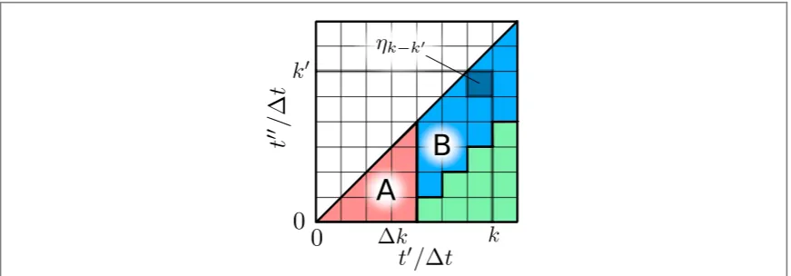
In its current form equation(6)is, in principle, numerically computable, though would require the storage of theD2Nnumbers making up the discretized influence functional. The exponential dependence of storage requirements on the number of timesteps places strict limits on the length of time for which a given simulation can be propagated. To circumvent this issue we make use of thefinite memory approximationoriginally introduced by Makri and Makarov[32,33]. For a continuum of bath oscillator modes the correlation function equation(11)decays at worst algebraically and infinite time becomes effectively zero. This in turn implies that the coefficientsh_{k k- ¢}decay to zero as the differencetk-tk¢is increased. Thefinite memory approximation

involves setting those coefficients for whichk- ¢ > Dk ksuch that the time differencetk-tk¢> D D ºk t tc

identically equal to zero. Here we have introducedtc, the bath cutoff time, which must be suitably large to ensure

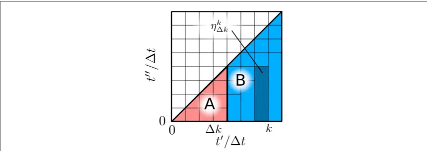
converged results. Infigure1we visualise this memory cutoff in terms of two dimensional integral regions over

¢ - 

( )

C t t . Forfixedkthe coefficientsh_{k k- ¢}correspond to columns of a numberDksquare integral regions extending up to the triangular regions which giveh₀. Thefinite memory approximation is then made by setting all of the coefficients in the green region to zero. This has the effect that the dynamics we calculate in region A are exact and the approximation only affects what happens for timest>tc+ Dt.

With thefinite memory approximation we can now reformulate equation(6)in terms of the iterative propagation of an object known as the ADT(as before). This propagation is computationally realised most efficiently as contractions between multidimensional tensors but the analogy to standard density matrix propagation is most easily seen by representing it as operator-vector multiplication in an augmented Liouville space:



r +t ññ = t r ññ

∣ _RA(t c) e ∣ _RA( )t , (13)

A c

where∣r_RAññis the vectorized ADT andA_{is the augmented Liouvillian. The augmented space is constructed by}

taking the product ofDkcopies of the original Hilbert space. The basis of this space at a given timetkis

constructed by taking a product of reduced system basis states at that time and the previousD -k 1times

¼

- -D +

tk 1 tk k 1

ññ = ññ -ññ ¼ -D +ññ

∣SkA ∣Sk ∣Sk 1 ∣Sk k 1 , (14)

thus giving the augmented Hilbert space a dimension ofD2Dk_{. The information stored in the ADT is a set of}

amplitudes weighting each of the trajectories the reduced system could have taken through its Hilbert space in the previousDktimesteps of the evolution. The physical reduced density matrix at a given time is then found by summing these amplitudes:

å

r ññ = áá ¼ áá r ññ

¼

- -D +

- -D +

∣ _R( )tk S ∣ S ∣ ( )t . (15)

S S

k 1 k k 1 _RA k

k 1 k k 1

Computing equation(6)with the memory cutoff requires the storage of theD2Dk_{elements of the vector}

representing the augmented state and theD4Dk_{elements of the propagator matrix. As mentioned above this is}

not the optimal representation for actually carrying out the propagation; in fact the alternative tensor

representation of the propagator only has_D2(D +k 1)_{elements. In theappendixwe explicitly construct this more}

efficient tensor propagation and also give the matrix elements of the propagator,ááSkA∣ eA ct∣SkA_-Dkññ, as well as

the components of the initial augmented state vector,ááSDk∣r tR( )ññ

A A

c , required for both tensor and matrix

representations of the method.

The scheme then has two parameters which need to be adjusted to ensure convergence of results. The memory cutoff time,tc, should be made large enough, by increasingDk, such that increasing it any further has

negligible effects on thefinal result. At the same time the error induced by the Trotter splitting must also be eliminated by decreasing the timestepDt, which in turn decreasestcfor a givenDk. Thus, achieving the best

results requires both maintaining a small enough timestepDtto eliminate the Trotter error while at the same time keeping it large enough such that the number of timesteps required to capture the correlation time of the bath is kept as small as possible. Details on the method forfinding the optimal value ofDtthat minimises the overall error can be found in[43].

Finally, we note that the ADT has many properties in common with a standard density matrix: it is both Hermitian and has unit trace, from which it follows that a system density matrix calculated from it is also guaranteed to have these properties. To describe a physical state it is also necessary that the system density matrix is positive. Proving this is, in general, more difficult and it is known that the ADT scheme does not guarantee positivity of the reduced system state[57]. In the following section we will gain an understanding of how non-positive reduced system states can occur and describe a procedure to help prevent this from happening.

3. Memory cutoff in an exactly soluble model

To investigate the role of thefinite memory approximation in the occurrence of non-positive reduced system states, here we study the effects of making this approximation on an exactly soluble pure dephasing model where

=

[H s0, ˆ] 0. The simplest example of such a model is that of a two level system described by the Hamiltonian

s

=

H0 z 2which couples to the bath viasˆ=sz. This is theindependent boson model[2]which we will use as an

example here. Note however that what follows can be applied to any model which satisfies the commutation relation above.

3.1. Independent boson model

For this model the Trotter splitting in equation(5)is exact since the system and bath Hamiltonians commute. Also, by moving to the interaction picture of the reduced system we may ignore the dynamics induced byH0and

the free system propagator is therefore the identity

 _{d d}

áá D ññ = áá ñññ =

- - +

-+

-∣ ∣ ∣ ( )

Sk e 0 tSk 1 S Sk k 1 s s_{k k} 1 s sk k 1. 16

The summation in equation(6)can now be carried out exactly(without thefinite memory approximation)to obtain

r r

áá_{S ∣ ( )t} ññ =_eG( )áá_{S ∣} ññ_{, (17)}

N R N S tN N, N 0

where

h h

G = -

--

-+ -+

-( ) ( ) [ ( )]

(( ) ( ) ) [ ( )] ( )

S t s s t

s s t

, Re

i Im . 18

N N N N N

N N N

2 2 2

Here we have defined the function

ò ò

å å

h = h = ¢ -   ¢

= ¢= - ¢

¢

( )tN C t( t )d d ,t t (19)

k N

k k

k k

t t

0 0 0 0

N

which governs all dynamics induced by the interaction with the bath. We see that state populations on the diagonal ofr_R( )t (wheres+=s-)do not undergo evolution and all dynamics are in the decay and oscillations of the coherences.

In what follows we examine the effect of making thefinite memory approximation on the functionh( )t . Note that this also describes the effects of making this approximation on the discretized influence functional since thehk k- ¢coefficients can be written entirely in terms of this function,

h h h h

h

= - + ¹ ¢

= ¢

- ¢ - ¢+ - ¢ -

¢-⎧ ⎨ ⎩

( ) ( ) ( )

( ) ( )

t t t k k

t k k

2

. 20

k k

k k 1 k k k k 1

To work out how the solution is changed when we impose the memory cutoff we must consider what happens to the functionh( )t when we remove those coefficients for whichk- ¢ > Dk kfrom the sum in equation(19). Infigure1we see there are two distinct regions of the integral domain left after performing the memory cutoff: whent<tc+ Dt,(region A)ηis unaffected by the cutoff and region B wheret>tc+ Dtand

at least some correlations are cutoff. The sum of the coefficients within region A is exactlyh t( c+ Dt), while using equation(20)the sum of all the coefficients in a single strip of region B ish t( c+ D -t) h t( )c . There are

D

-N k 1of these strips in total and so by summing up all coefficients remaining after thefinite memory approximation wefind the functionh( )t is approximated as

h »h t + -t h t + D -h t

D

( )t ( ) (t ) ( t) ( ) ( )

t . 21

c c c c

This result can also be obtained in theD t 0limit by settingC t( )=0fort >tcin the integral of

equation(19). By making a change of variables= ¢ - t t , wefind

ò ò

h( )t = ¢ C s( )d ds t¢ (22)

t t

0 0

ò ò

ò ò

» t ¢ + ¢

t t

¢

( ) ( ) ( )

C s d ds t C s d ds t 23

t t

0 0 0

c

c c

h t t h t

= ( )c +(t- c) ˙ ( )c , (24)

where the dot indicates a time derivative. Thus the dynamics of the pure dephasing model with thefinite memory approximation imposed are as follows: at timest tc+ Dtthe exact dynamics are followed. While

fort >tc+ Dtthere is an exponential decay with rategc=Re[ ˙ ( )]h tc accompanied by a Lamb-shift of the

system frequencies,L =c Im[ ˙ ( )]h tc .

It is easy to see now how a problem can arise if the memory cutoff is at a point where the gradient ofh( )t is negative. The resultant decay rate is negative and hence there is exponential growth of all coherences fort >tc.

This inevitably leads to the system density matrix becoming non-positive.

Additionally, unlessRe[ ˙ ( )]h tc =0identically,finite steady state coherences will be impossible to produce. Increasingtcincreases the time it takes for the coherences to decay or grow away from the true steady state, but

forfinitetcthe convergence of thefinite memory approximation, and hence the ADT scheme, cannot be

guaranteed at arbitrary times.

To investigate how these problems manifest in the dynamics of a real example we need to specify the environmental coupling, quantified by the spectral densityJ( )w , which determines the form ofh( )t . We consider the spectral density

w a w

w

= _nn w w

-

-( ) ( )

J

2 _c 1e , 25

c

which is characterised by the dimensionless coupling constant,α, ohmicity,νand an exponential cutoff at a scale given bywc. It has been found that the general condition forh˙ ( )t >0is that the functionJ( )w coth(w 2T) w2

be convex, and that for spectral densities of the form equation(25)this condition is fulfilled whenn <ncritfor

some critical ohmicityncrit[61]. The value ofncritvaries monotonically fromncrit=2andncrit=3as

temperature is increased from 0 to¥. Negative decay rates arise whenn>ncrit. Therefore atT=0 it is in the

superohmic regime, wheren>2, that we expect tofind thefinite memory cutoff results in non-positive dynamics. To demonstrate this we plot infigure2the time dependent decay rate resulting from both ohmic and superohmic spectral densities at zero temperature. We also plot the resultant dynamics of the coherence, for both the exact solution of the independent boson model, equation(17), and with the memory cutoff imposed. In this case the imaginary part of the exponential in equation(17)disappears, since the eigenvalues ofsˆhave equal magnitude, so the dynamics are that of pure decay. For the ohmic case the decay rate is always positive and using the memory cutoff produces exponential decay to the correct steady-state of zero coherence. There is still a significant discrepancy at intermediate times, but this can be reduced by increasingtc. For a superohmic spectral

density there is a large window of time when the decay is negative. Making the cutoff in this window results in unphysical dynamics with exponential growth. Notably, in this superohmic case the decay rate approaches zero from below asymptotically. This means that increasingtcdoes not remove this spurious asymptotic behaviour,

it just shifts its onset to longer and longer times.

To conclude this analysis we point out a situation in which even the ohmic and sub-ohmic regimes 

n

<

0 2can display negative decay rates and hence non-positive states. In constructing physically realistic models one may want to account for how spatially separated states interact with the same bath of oscillators. For the case of the two-level independent boson model considered above in three dimensions the spatial separation of the two system eigenstates is accounted for via a multiplicative correction to the spectral density

w

equation(25)go asJ( )w µwn+ -2e w wc_{and the effective critical ohmicity for the transition to non-Markovian} dynamics with negative decay rates now lies in the range0<ncrit1and the potential for the memory cutoff to produce unphysical dynamics exists for all values ofν.

3.2. Fixing the non-positive evolution

We now seek a way of taking the memory cutoff such that the exact solution equation(17)is always reproduced using the ADT method. A general way to do this would be to define a new set of the coefficientsh˜k k_{- ¢},



- ¢ D

k k kin such a way that their sum is constrained as follows,

å å

å å

= ¢= -D - ¢ = ¢= - ¢

˜ ( )t , (26)

k N

k k k

k

k k k

N

k k

k k

0 0 0

thus reproducing the exact dynamics governed byh( )t , independent of bothtcandDt. It seems reasonable that

we should attempt to redefine as few of the coefficients as possible, since they already exactly account for non-Markovian correlations within a timespantc(up to the Trotter error). The key idea behind thefinite memory

cutoff is that the most non-local temporal correlations in the system are the most insignificant, hence∣h_{k k- ¢}∣»0 for largek- ¢k. Thus we redefine only the coefficients with the largestk- ¢ = Dk kas follows

å

h h h h

h

= + º - ¢ = D

- ¢ < D

- ¢ - ¢ = D

-- D - ¢

⎧ ⎨ ⎪

⎩ ⎪

˜ k k k ( )

k k k.

27

k k

k k j

k k

k j k

k

k k

0 1

This redefinition will not introduce any problems as long as∣h_{k k- ¢}∣»∣ ˜h_{k k- ¢}∣which is true sincetcis already

large enough to naïvely justify thefinite memory approximation. This redefinition is visualised infigure3in a similar way to the standard memory cutoff infigure1. From this schematic one can identify that this redefinition

corresponds to extending the lower limit of the integral down to zero. This means that it is straightforward to calculate the redefined coefficient:

ò ò

h h h t h t

= ¢ -   ¢

= - - + - D

t

D

-( )

( ) ( ) ( ) ( ) ( )

C t t t t

t t t

d d

. 28

k k

t

t t

k k

0

1 c c

k k k

1 c

In terms of implementing the ADT scheme the main consequence is that now a new propagator must be

constructed at every step of the iterative propagation, though the actual structure of each propagator is essentially identical to the original. Thus, although slightly more time consuming, carrying out the propagation is no more complicated than before. The time-dependence in our method is fundamentally different from that generated

Figure 2.The decay rateh˙ ( )t and dynamicsexp(-4 Re[ ( )])h t forn=1,n=3, in red and blue, respectively, for exact results

(dotted)and with the memory cutoff(dashed). The vertical lines indicate the memory cutoff timew tc c=2.5and other parameters

by time-dependent Hamiltonians, in that it is due to the non-local influence of the bath interaction itself. In the standardfinite memory approximation thefinite ranged non-Markovian correlations allow the problem to be reformulated as one with Markovian evolution but in a higher dimensional augmented Hilbert space as in equation(13). We have gone one step further by allowingAto be time-dependent, thus allowing transient

non-positive evolution of the reduced system state beyond the cutoff timetcwhile still maintaining overall positive

evolution from the initial state. This is not possible in the standard ADT scheme where the augmented

Liouvillian is time-independent and so must have no positive eigenvalues to ensure positive evolution. We point out here that the instability of steady states and non-positivity in the ADT scheme for superohmic environments has been recognised before, and a similar redefinition of theh_{k k- ¢}coefficients has been proposed[57,58]but only in a way that gives qualitatively correct asymptotic behaviour of the pure dephasing model above, but does not reproduce the exact solution identically.

In the following section we show that this new method is useful for more complicated models which do not have an exact solution by applying it to the more general spin-boson model.

4. Application to the spin-boson model

The spin-boson model[62]provides a paradigmatic example of an open quantum system and can be used to model a wide variety of physical systems. For example, it has been applied to the problem of electron transfer in biological aggregates[63], exciton dynamics in quantum dots[4], transport in mesoscopic systems[64]and chemical reactions[65]. The system Hamiltonian isH0=sz+Vsxand the coupling to the environment is

through the operatorsˆ=sz. Hereòagain gives the energy splitting of the two levels, while thesxterm generates

coherent transitions between the two states. The addition of thissxterm breaks the integrability of the

independent boson model and allows for a rich variety of physics to be explored.

In what follows we will be particularly interested in the case where the environment is superohmic, since this is where we found the most pathological behaviour in the independent boson model. The superohmic regime is most studied in the context of quantum dots strongly coupled to a phononic environment[4,5,66]. For many parameters a polaron master equation provides a successful route to capturing non-perturbative effects[19], but for highly non-Markovian environments this approach fails. Here we show how the ADT scheme is able to capture backflow of energy from the environment to the system in this regime.

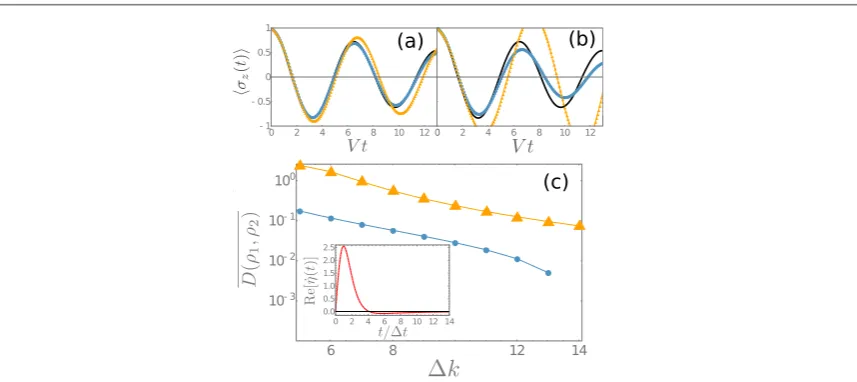
To show the improvement gained by the new integration scheme which we detailed in the previous section, we show how the convergence of the results withDkchanges as compared to the standard approach. Infigure4

we study the spin-boson model with=0at zero temperature with a large reservoir cutoff frequency

wc V=5. Tofind an approximation for the error in our results we compare everything to the most converged case: that using the new memory cutoff atD =k 14. We then calculate the time average of the trace distance[67]

between these converged results and each other case. The trace distance is given by

r r = r -r

( ( ) ( )) ∣ ( ) ( )∣ ( )

D t , t 1 t t

2Tr , 29

1 2 1 2

where where∣ ∣_A = _AA†_{,r( )t}

1 is the converged density matrix andr2( )t is the density matrix we want to

compare tor₁( )t . We show this deviation as a function ofDkfor both approaches in the panel(c)offigure4. We see that our new approach converges much more quickly than the standardfinite memory approximation: by

D =k 11the errors in the new approach are negligible while the standardfinite memory approximation still has significant errors atD =k 14. This can also be seen in the dynamics infigures4(a)and(b)where we see that our new approach converges much more quickly when increasingDk.

It is difficult tofind convergence with this set of parameters because the gradient ofh( )t approaches zero from below(as can be seen in the inset tofigure4(c))and so the problems we found for the independent boson model still occur, although here they are less severe and the standard approach only gives unphysical results at very smallDk.This problem becomes even worse if we move further towards the so-called scaling limit of the model[62], wherewcis the largest energy scale in the problem, by increasing the value ofwc. This means a

smaller requiredtc, but also results in a larger magnitude ofh t˙ ( )c so that the timescale for the onset of divergent

dynamics becomes much shorter and achieving convergence over appreciable lengths of time becomes very difficult.

Now we have shown the improvement gained by our improved memory cutoff we examine in detail the dynamics of the spin-boson model in a parameter regime which is difficult to access using the standard memory cutoff approximation: when there is non-Markovian behaviour far from the scaling limit with a lower cutoff frequencywc V=1and atfinite temperature. In this limit the required value ofDkwithout our improvement would be much too large to store in memory for a standard computer.

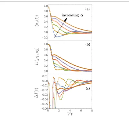
Infigure5(a)we show the population difference dynamics with initially excited spin,r₀= ñá∣1 1∣, for system-bath couplings between0.5<a<1.9. At low coupling strengths we see simple damped oscillations, as would be captured by a weak coupling master equation. Increasing the coupling changes these oscillations from underdamped to overdamped, as would be found using for example a polaron master equation. However, the overdamped regime is accompanied by a highly non-Markovian feature: a revival of the population difference which becomes more pronounced at stronger couplings.

In order to establish a more concrete quantification of the non-Markovian nature of these dynamics we examine how distinguishable two distinct initial states are as they evolve in time. To do this we again use the trace distanceD( ( )r₁t ,r₂( ))t as a natural measure. For a Markovian system as time evolves all states move closer to the steady state and so asymptotically we expectlimt¥r1( )t =limt¥r2( )t =rsteady, provided the steady

stater_steadyis unique. This means thatD( ( )r₁ t ,r₂( ))t monotonically decays to zero for any two initial states. If, however, the dynamics are non-Markovian then, for certain pairs of initial states, there can be increases in the trace distance as a function of time as the environment allows information toflow back into the system. It is therefore evident that quantity of interest is actually

r r

DI t( )= ( ( ) ( )) ( )

tD t t

d

d 1 , 2 , 30

which is positive when these non-Markovian features occur.

Infigures5(b)and(c)we show the trace distance andDI t( ), for the same set of parameters as in(a), using the orthogonal initial statesr₁( )t = ñá∣1 1∣andr₂( )t = - ñá-∣ 1 1∣. At low values of coupling there are weak oscillations inDI t( )between negative and positive which are damped and pushed out to longer times as the

Figure 4.Top panels: dynamics of the spin-boson model for(a)D =k 11and(b)D =k 6compared to the converged results(black) for the improved memory approximation(blue)and the standard ADT(orange). Panel(c): the trace distance between the converged result against the value ofDkused for the standardfinite memory approximation(orange triangles)and our improved memory approximation(blue dots). The inset shows the time dependent decay function. Parameters in all panels area=0.7,wc V=5,

coupling is increased. Increasing the coupling still further leads to an additional positive region ofDI t( )at short times, which remains there, closely following the early time revival we see in the population differences in figure5. This observation confirms that this feature is a signature of information backflow. Similar features have been observed in biased spin-boson models(i.e.¹0)[24,51,68]. Here, we show quantitatively that non-Markovian features are present in the dynamics of the unbiased spin-boson model.

To analyse the dependence of the non-Markovian revival in the population dynamics on the parameters describing the bath wefit the dynamics to the sum of two decaying oscillations:

a _{( )t} =_Ae-g _cos(w_t)+_Be-g _sin(w _t +f_{), (31)}

z 1t 1 2t 2

with the constraintaz( )0 =A + Bsin( )f =1. The frequencyw1and decay rateg₁parameters capture the

weak-coupling and long time dynamics, whilew2andg₂describe the higher frequency short time dynamics of

the revival. An example of one of thesefits, fora=0.6, is shown in the inset tofigure6.

We show howg₂ Vandw2 Vvary as the coupling to the bath,α, is increased infigure6(a). Bothg2 Vand

w2 Vincrease with coupling at roughly the same rate and, although the behaviour is certainly not linear, this

dependence implies that increasing coupling simply causes the timescale over which the revival occurs to shorten. This is consistent with the revival being due to a backflow of information from the bath: we would expect larger couplings to simultaneously cause quicker information backflow and to wash it out more quickly. Infigure6(b)we show what happens as the temperature of the bath is changed. Increasing temperature both increases the effective coupling to the bath but also scrambles temporal correlations, reducing the bath correlation time. Therefore we see both the damping and frequency of the revival increase with increasing temperature.

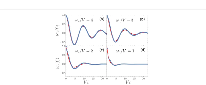
Before concluding, we compare the results above to those obtained using a Markovian polaron master equation[19]. If our interpretation of the revival is correct, then it is obvious that any approach which does not fully account for the dynamics of the bath will be unable to reproduce this feature. For example, the population

Figure 5.₍a₎Population difference dynamics for various values of coupling strength to the batha=0.5, 0.7, 1, 1.3, 1.6, 1.9.

difference dynamics predicted using the polaron master equation are of the same form as equation(31)but with g₁=g₂andw1=w2[19,20]. This is shown infigure7. For the largest values ofwcin(a)and(b)the system is in

the scaling limit[62], where the polaron technique works well, and indeed wefind good agreement of the two methods, with only small deviations occurring at very short timescales. Aswcdecreases, we enter a more

non-Markovian regime and we see that the polaron master equation starts to fail. It is difficult tofind converged results which show this effect more clearly than shown here, since in the scaling limit divergent dynamics occur on very short timescales, as discussed earlier. The long time dynamics predicted by the polaron equation are qualitatively correct, taking the form of an exponentially decaying oscillation, but as anticipated it completely fails to capture the non-Markovian revival which we found above using the improved ADT. We attribute this to the breakdown of the Markov approximation used in deriving the polaron master equation. From our earlier discussion, we know that the revival in dynamics is most prominent for smaller values ofwc, i.e. for baths with

longer correlation times. This, together with the poor agreement of ADT with the polaron master equation at short times, confirms our conclusion that this feature is a highly non-Markovian effect which could not be produced using any form of time-local master equation.

5. Summary

We have shown how the standardfinite memory approximation in the ADT numerical scheme can cause unphysical behaviour resulting in periods of non-positive evolution. We have provided an improvement to this method which is able to reproduce the exact solution to the pure dephasng model. To demonstrate the

applicability of this new method we have shown converged results for dynamics of the symmetric spin-boson model in a superohmic environment. We found that our new method is able to reach convergence using significantly smaller computational resources than the standardfinite memory approximation. At strong system-bath coupling strengths in this regime we found highly non-Markovian revivals in the dynamics which are accompanied by non-monotonicity of the trace distance between different initial states. These features are not present in simpler analytical approaches such as polaron master equations.

Figure 6.The decayg₂ V₍purple dots₎and frequencyw2 V(green squares)fitting parameters corresponding to the high frequency

sinusoidal oscillation present on top of the decaying cosine. In(a)these are plotted against dimensionless couplingαwith wc V=T V=1. In(b)these are plotted against temperature withwc V=a=1. The inset shows an example of thefit to

equation(31) (blue solid line)compared to the numerical results(red dots)ata=1.

Figure 7.Population difference plotted using the ADT with our improved memory cutoff(blue dots)and the polaron master equation

Acknowledgments

We acknowledge useful discussions with EMGauger. We thank D P S McCutcheon for providing the code used for the polaron simulations. AS acknowledges a studentship from EPSRC(EP/L505079/1). BWL

acknowledges support from EPSRC(EP/K025562/1). PGK acknowledges support from EPSRC(EP/M010910/ 1). The research data supporting this publication can be found at:http://doi.org/10.17630/

21764101-6493-46e7-ab85-65cccc1fb9e5.

Appendix. Explicit construction of propagation methods

We start by rewriting the summand of equation(6)in the following form



 

= áá ññ

= ¢= ¢ D ⎛ ⎝ ⎜⎜ ⎞_⎠⎟⎟ ({ }) ({ }) ˜( ) ∣ ∣ ( )

F Sk I Sk I S S, S e S , A1

j N

j j

j j t

1 1

1 0 0

where



= - ¢ ¹

áá ññ - ¢ =

f f ¢ -D ¢ -¢ ¢ ⎪ ⎪ ⎧ ⎨ ⎩ ˜( ) ∣ ∣ ( ) ( ) ( )

I S S j j

S S j j

, e 1

e e 1, A2

j j

S S

j t j S S

, , j j j j 0 with *

f(S Sj, j¢)=(sj+-s-j)(s+j¢hj j- ¢-s-j¢hj j- ¢). (A3)

There is noS0dependence in any of theI S S˜( k, k¢)so theS0summation in equation(6)can be carried out,

propagating the reduced system for a timeDtunder the free Liouvillian0into the staterR(Dt). Thefinite

memory approximation, settingh_{k k- ¢}=0fork- ¢ > Dk k, then translates toI S S˜( k, k¢)=1fork- ¢ > Dk k. This allows the product overI S S˜( k, k¢)ʼs to be rewritten as

 



= ¢=

¢

=D +

- -D D D

-˜( ) ( ) ( ) ( )

I S S, S S, S A S ,S S , A4

j N j j j j j k N

j j j k k k

1 1 1

1 1 1

where we have defined



L - ¼ -D =

= D

-(S Sj, j Sj k) I S S˜( , ), (A5)

m k

j j m

1

0

to be the elements of the propagator tensor, and

 

¼ = áá D ññ

D D

-= D

¢=

¢

( ) ∣ ( ) ˜( ) ( )

A S k,S k S S R t I S S, , A6

k k

k k

k k

1 1 1

1 1

to be the elements of the initial ADT. The summations over theSkcan now be carried out one at a time by

iteratively multiplying and contracting tensors:

å

¼ = L ¼ ¼

- -D + - -D - - -D

-D

( ) ( ) ( ) ( )

A S Sk, k Sk k S S, S A S ,S S , A7

S

k k k k k k k k

1 1 1 1 2

k k

with the initial condition equation(A6). The reduced system density matrix at a timetkis then retrieved by

summing over all but theSkindex

å

áá ññ = ¼

¼

- -D +

- -D +

∣ ( ) ( ) ( )

Sk R tk A S S, S . A8

S S

k k 1 k k 1

k 1 k k 1

The propagator tensor equation(A5)hasD +k 1indices and so has_D2(D +k 1)_{elements, making the tensor}

contraction representation of the propagation less demanding than representing the augmented state as a vector and propagating with aD4Dk_{sized matrix. Within the Liouvillian matrix formalism for propagation,}

equation(13), and using the basis defined in equation(14), the elements of the augmented state at a timetkare r

ááSk∣ R( )tkññ =A S S( k, k- ¼Sk-D +k ) (A9)

A A

1 1

and the matrix elements of the propagator across the timespantchave the simple analytic form



_

áá t ññ = L ¼

-D

= -D +

- -D

∣ ∣ ( ) ( )

Sk e Sk k S S, S . A10

j k k

k

j j j k

A A

1

1

Thus another way of solving the problem would be to construct and diagonalize this propagator tofind the eigenvectors of the augmented LiouvillianA_{, though for typical valuesD ~k 10it is much more efficient to use}

the iterative propagation schemes above.

ORCID iDs

B W Lovett https://orcid.org/0000-0001-5142-9585

References

[1]Chirolli L and Burkard G 2008Adv. Phys.57225

[2]Breuer H-P and Petruccione F 2002The Theory of Open Quantum Systems(Oxford: Oxford University Press)

[3]Madsen K H, Ates S, Lund-Hansen T, Löffler A, Reitzenstein S, Forchel A and Lodahl P 2011Phys. Rev. Lett.106233601

[4]Ramsay A J, Gopal A V, Gauger E M, Nazir A, Lovett B W, Fox A M and Skolnick M S 2010Phys. Rev. Lett.104017402

[5]Ramsay A J, Godden T M, Boyle S J, Gauger E M, Nazir A, Lovett B W, Fox A M and Skolnick M S 2010Phys. Rev. Lett.105177402

[6_]Wilson-Rae I and Imamo_ğlu A 2002Phys. Rev.B65235311

[7]McCutcheon D P S 2016Phys. Rev.A93022119

[8]Stanwix P L, Pham L M, Maze J R, Le Sage D, Yeung T K, Cappellaro P, Hemmer P R, Yacoby A, Lukin M D and Walsworth R L 2010 Phys. Rev.B82201201

[9]Wang Z-H and Takahashi S 2013Phys. Rev.B87115122

[10]Liu B-H, Li L, Huang Y-F, Li C-F, Guo G-C, Laine E-M, Breuer H-P and Piilo J 2011Nat. Phys.7931

[11]Bylicka B, Chruściński D and Maniscalco S 2014Sci. Rep.45720

[12]Rivas A, Huelga S F and Plenio M B 2010Phys. Rev. Lett.105050403

[13]Feynman R P and Vernon F L 1963Ann. Phys.24118

[14]Feynman R P and Hibbs A R 1965Quantum Mechanics and Path Integrals(New York: McGraw-Hill)

[15]Caldeira A and Leggett A 1983PhysicaA121587

[16]Weiss U 2012Quantum Dissipative Systems(Singapore: World Scientific)

[17]Breuer H-P, Laine E-M and Piilo J 2009Phys. Rev. Lett.103210401

[18]Lindblad G 1976Commun. Math. Phys.48119

[19]Nazir A and McCutcheon D P S 2016J. Phys.: Condens. Matter28103002

[20]McCutcheon D P S and Nazir A 2011Phys. Rev.B83165101

[21]Roy C and Hughes S 2012Phys. Rev.B85115309

[22_]Pollock F A, McCutcheon D P S, Lovett B W, Gauger E M and Nazir A 2013New J. Phys.15075018

[23_]Jang S, Cheng Y-C, Reichman D R and Eaves J D 2008J. Chem. Phys.129101104

[24]Jang S 2009J. Chem. Phys.131164101

[25]Marthaler M, Utsumi Y, Golubev D, Shnirman A and Schön G 2011Phys. Rev. Lett.107093901

[26]Kolli A, O’Reilly E J, Scholes G D and Olaya-Castro A 2012J. Chem. Phys.137174109

[27]Zimanyi E N and Silbey R J 2012Phil. Trans. R. Soc.A3703620

[28]Kirton P and Keeling J 2013Phys. Rev. Lett.111100404

[29]Kirton P and Keeling J 2015Phys. Rev.A91033826

[30]Iles-Smith J, Lambert N and Nazir A 2014Phys. Rev.A90032114

[31]Müller C and Stace T M 2017Phys. Rev.A95013847

[32]Makri N and Makarov D E 1995J. Chem. Phys.1024600

[33]Makri N and Makarov D E 1995J. Chem. Phys.1024611

[34]Sim E 2001J. Chem. Phys.1154450

[35]Makri N 2017J. Chem. Phys.146134101

[36]Shao J and Makri N 2002J. Chem. Phys.116507

[37]Nalbach P, Eckel J and Thorwart M 2010New J. Phys.12065043

[38]Barth A M, Vagov A and Axt V M 2016Phys. Rev.B94125439

[39]Chang H-T, Zhang P-P and Cheng Y-C 2013J. Chem. Phys.139224112

[40_]McCutcheon D P S, Dattani N S, Gauger E M, Lovett B W and Nazir A 2011Phys. Rev.B84081305

[41_]Nalbach P and Thorwart M 2010Phys. Rev.B81054308

[42]Thorwart M, Eckel J and Mucciolo E R 2005Phys. Rev.B72235320

[43]Eckel J, Weiss S and Thorwart M 2006Eur. Phys. J.B5391

[44]Cygorek M, Barth A M, Ungar F and Axt V M 2017 arXiv:1704.03347

[45]Tanimura Y and Kubo R 1989J. Phys. Soc. Japan58101

[46]Anders F B and Schiller A 2005Phys. Rev. Lett.95196801

[47]Bulla R, Lee H-J, Tong N-H and Vojta M 2005Phys. Rev.B71045122

[48]Anders F B, Bulla R and Vojta M 2007Phys. Rev. Lett.98210402

[49]Bulla R, Costi T A and Pruschke T 2008Rev. Mod. Phys.80395

[50]Yao Y, Duan L, Lü Z, Wu C-Q and Zhao Y 2013Phys. Rev.E88023303

[51]Prior J, Chin A W, Huelga S F and Plenio M B 2010Phys. Rev. Lett.105050404

[52]Egger R and Mak C H 1994Phys. Rev.B5015210

[53]Kast D and Ankerhold J 2013Phys. Rev. Lett.110010402

[54]de Vega I and Alonso D 2017Rev. Mod. Phys.89015001

[55]Nalbach P, Ishizaki A, Fleming G R and Thorwart M 2011New J. Phys.13063040

[56]Thorwart M, Reimann P and Hänggi P 2000Phys. Rev.E625808

[57_]Vagov A, Croitoru M D, Glässl M, Axt V M and Kuhn T 2011Phys. Rev.B83094303

[58_]Nahri1 D G, Mathkoor F H A and Ooi C H R 2016J. Phys.: Condens. Matter29055701

[60_]Suzuki M 1976Commun. Math. Phys.51183

[61_]Haikka P, Johnson T H and Maniscalco S 2013Phys. Rev.A87010103

[62]Leggett A J, Chakravarty S, Dorsey A T, Fisher M P A, Garg A and Zwerger W 1987Rev. Mod. Phys.591

[63]Xu D and Schulten K 1994Chem. Phys.18291

[64]Brandes T 2005Phys. Rep.408315

[65]Garg A, Onuchic J N and Ambegaokar V 1985J. Chem. Phys.834491

[66]Kok P and Lovett B W 2010Introduction to Optical Quantum Information Processing(Cambridge: Cambridge University Press)

[67]Breuer H-P, Laine E-M, Piilo J and Vacchini B 2016Rev. Mod. Phys.88021002