ISSN Online: 1947-394X ISSN Print: 1947-3931
DOI: 10.4236/eng.2019.1111050 Nov. 15, 2019 759 Engineering
Thermal Modeling of a Multilayer Integrated LC
Filter for Temperature Distribution Calculation
Somo Coulibaly
1, Diby Kadjo Ambroise
2, Loum Georges
11Institut National Polytechnique, UMRI EEA (LARIT-SISE), Yamoussoukro, Ivory Coast 2Université Félix Houphouët-Boigny, SSMT (LPMCT), Abidjan, Ivory Coast
Abstract
Thermal behavior of integrated passive components has become an impor-tant issue when designing these components. This paper presents the thermal modeling of a multilayer integrated LC filter used in DC-DC step-down con-verter for temperature distribution calculation. The approach used for this analysis is based on thermal equivalent circuit. Temperature distribution is obtained from algebraic equation, which is in vector and matrix form. The results of analytical calculation are compared with simulation results from fi-nite element method. These results showed a good correlation.
Keywords
Thermal Modeling, Integrated LC Filter, Temperature Distribution, F. E. M. Simulation
1. Introduction
Thermal design of electronic components and systems is to ensure that the tem-perature rise caused by the losses remains within acceptable limits. In power electronic converter, temperature causes around 54% of all the converter fail-ure [1]. It is therefore necessary to investigate the structures of the integrated LC passive module thermally to guarantee reliable operation of the integrated power module. Thermal modeling and simulation have become essential parts in process design. These integrated components are essentially magnetic compo-nents. Modeling these components provide good study of investigation of the temperature evolution through the integrated component.
However, modeling magnetic components requires knowledge of electromag-netic losses. These losses are due to current flow in the windings (“copper losses”), to the temporal variation of the magnetic field in the magnetic cores (“iron
How to cite this paper: Coulibaly, S., Am-broise, D.K. and Georges, L. (2019) Thermal Modeling of a Multilayer Integrated LC Filter for Temperature Distribution Calculation. Engineering, 11, 759-767.
https://doi.org/10.4236/eng.2019.1111050
Received: October 1, 2019 Accepted: November 12, 2019 Published: November 15, 2019
Copyright © 2019 by author(s) and Scientific Research Publishing Inc. This work is licensed under the Creative Commons Attribution International License (CC BY 4.0).
DOI: 10.4236/eng.2019.1111050 760 Engineering
2. Integrated LC Filter Overview
The studied integrated LC filter is shown in Figure 1[2] [3]. It consists of a PCB planar inductor sandwiched between two ferrite layers, and a capacitive part made of ferrite multilayer capacitors. The ferrite layers are flexible ferrite sheets used for both inductor magnetic core and capacitor dielectric medium. Inductor and capacitor parts are stacked together in series connection to give the inte-grated LC component.
3. Thermal Modeling of the Integrated LC Filter
The thermal analysis of an integrated component consists of studying its ability to evacuate heat to the outside. The purpose of such a study is to predict the risks of overheating of the different materials.
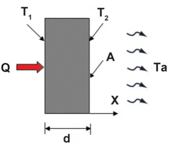
If one side of a solid is warmer than the other side, then heat flow goes through the body from the warmer side to the cooler one. Heat flow mechanism through a solid material is illustrated by Figure 2. Difference temperature from inside the component to outside consists of heat conduction and heat convec-tion.
The rate of heat loss is given by [4]:
(
1 2)
1 2th
A T T T T Q
d R
λ ⋅ ⋅ − −
[image:2.595.258.523.495.706.2]= = (1)
DOI: 10.4236/eng.2019.1111050 761 Engineering Figure 2. Heat Flow illustration in a solid material.
where:
th d R
A λ
=
⋅ is the thermal resistance of the solid [K/W];
Q = the heat flow [W];
T1 and TL = the temperatures at the ends of the solid material [K]; d = the thickness crossed by the heat source [m];
A = the surface of the heat source [m2];
λ = the thermal conductivity of the material [W/(m·K)].
On the outside surface of the solid material, heat transfer is mainly heat con-vection which is conducted between air and the surface. It can be obtained based on the Newton’s law of cooling [4]:
(
)
f af a
th
T T Q h A T T
R
−
= ⋅ ⋅ − = (2)
where:
Q = rate of heat flow (W); 1
th R
h A
=
⋅ is the thermal resistance for convection (K/W);
h = convective heat transfer coefficient (W/m2K); A = cross sectional area (m2);
Tf = surface temperature (K); Ta = ambient temperature (K).
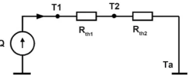
The thermal system of Figure 2 can be converted into an equivalent electrical system as shown in Figure 3 where voltage plays the same role as temperature (Equation (1)).
Rth1 is the thermal resistance of the solid for conduction; Rth2 is the thermal re-sistance for convection.
Since Q is constant throughout the network, it follows that:
2
1 2
1 2
a
th th
T T T T
Q
R R
− −
= = (3)
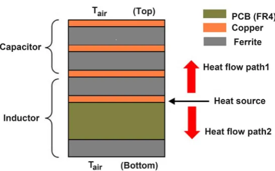
DOI: 10.4236/eng.2019.1111050 762 Engineering The heat source generated inside le component by the spiral winding copper is drained towards ambient air taking two dissipation paths as shown in Figure 4. In this representation, we considered that capacitor part of the integrated LC filter is made of two layers of ferrite material for demonstration purpose. In practice, number of ferrite layers depends on the value of capacitor.
Knowing the loss in the spiral winding, the thermal model must allow deter-mining the operating temperature in some points of the component along the heat flowing path.
Thermal modeling of an integrated multilayer structure is quite complex. To simplify the modeling of this component, we make a number of assumptions [5]:
Each layer must satisfy the heat conduction equation. Steady state conduction;
One-dimensional heat flow; Constant properties of materials;
Uniform heat flow in each layer; Perfect contact between layers;
Perfectly flat layers with uniform thickness;
Component boundaries (top and bottom faces) convect heat to the ambient on both sides.
From the cross section view of the structure shown in Figure 4, the equivalent thermal model of the structure can be represented as interconnection of the thermal resistance of each layer as in electrical circuit (Figure 5).
In this representation, Rthcu, Rthfe and RthFR4 stand for the thermal resistances of copper, ferrite and PCB layers, respectively.
The conduction path 1 consists of seven resistors: Rthcu/2 (resistance between the center of the conductor and its lower surface), Rthfe (resistance due to the fer-rite layer) and Rthcu (resistance due to the copper layer).
The conduction path 2 consists of two resistors: Rthcu/2 (resistance between the center of the conductor and its upper surface), RthFR4 (resistance due to the epoxy PCB) and Rthfe (resistance due to the ferrite layer).
[image:4.595.278.474.69.153.2]DOI: 10.4236/eng.2019.1111050 763 Engineering Figure 4. Cross section of the integrated LC component showing heat flow paths from heat source to the outside.
Figure 5. Integrated LC component thermal model.
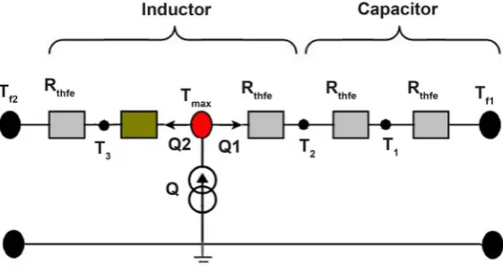
Because of the high thermal conductivity of the copper and its small thickness (35 μm), the temperature may be considered as uniform inside the spiral winding, and then Tcu and Tmax are equal. We can therefore neglect the thermal resistance Rthcu/2 on each side of Tmax. This leads to the reduced model circuit shown in
Figure 6.
The heat source Q generated by the copper spiral winding at the node Tmax is spread into two heat sources Q1 and Q2 such that Q = Q1 + Q2 because of energy conservation.
Finally, the problem is to determine temperatures Tmax, T1, T2, T3, Tf1 and Tf2 from the knowing thermal resistors Rthfe, RthFR4, Rthcu and the generated heat Q. Temperature Tair is fixed by forced or natural convection on both flat faces of the integrated LC component.
Under the above assumptions, temperature distribution can be calculated from the following equations:
(
)
(
)
1 fe max 2 fe 2 1
Q =K ⋅ T −T =K ⋅ T −T (4)
(
)
(
)
1 fe 2 1 fe 1 f1
Q =K ⋅ T −T =K ⋅ T −T (5)
(
)
(
)
1 fe 1 f1 f1 air
Q =K ⋅ T −T = ⋅ ⋅h A T −T (6)
(
)
(
)
2 FR4 max 3 fe 3 f2
Q =K ⋅ T −T =K ⋅ T −T (7)
(
)
(
)
2 fe 3 f2 f2 air
Q =K ⋅ T −T = ⋅ ⋅h A T −T (8)
(
)
(
)
4 max 3 max 2
FR fe
DOI: 10.4236/eng.2019.1111050 764 Engineering Figure 6. Reduced thermal model of integrated LC component.
where h [W/(m2·K)] is the coefficient of heat transfer by convection, A [m2] the area of the layers of materials, KFR4 and Kfe are defined as the thermal conduc-tance (inverse of thermal resisconduc-tance) of PCB and ferrite layers, respectively.
These simultaneous equations can be rearranged by putting unknown para-meters (Tf2, T3, Tmax, T2, T1, Tf1) on one side and the known ones on the other side. This leads to the matrix equation [Kth] × [T] = [F] represented by Equation (10) where Kth is matrix of thermal Conductance, T the unknown temperature vector and F the heat source vector.
(
)
2
3
max
4 2
1
4 4
0 0 2 0 0
0 0 0 2 0
0 0 0 0
0 0 0 0
0 0 0 0
0
0 0 0
fe fe fe f
fe fe fe
fe fe
air
fe fe FR
fe fe air
f
FR FR fe fe
K K K T
K K K T
K K T h A T
K K K T
K h A K T h A T
T
K K K K
− ⋅
− ⋅
− ⋅ ⋅
× =
− + ⋅ − ⋅ ⋅
− + −
(10) The unknown nodal temperatures are given by the following relation:
[ ]
[ ] [ ]
1th
T = K − ⋅ F (11)
The solution can be obtained by using numerical calculation software such as MATLAB.
4. Results and Discussions
To verify the solution of the analytical method, “Heat Flow Problem” module of FEMM software [6][7] has been used. The values of the properties of the mate-rials used in the design of the integrated LC filter are given in Table 1.
Calculated thermal resistance and their corresponding thermal conductance are given in Table 2.
DOI: 10.4236/eng.2019.1111050 765 Engineering Table 1. Thermal conductivity λ of different materials.
Material λ [W/mK)] Thickness (mm)
PCB_FR4 0.3 1.6
Copper 401 0.035
Ferrite 1.5 0.2
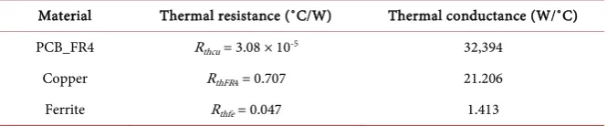
Table 2. Values of thermal resistance and corresponding thermal conductance.
Material Thermal resistance (˚C/W) Thermal conductance (W/˚C)
PCB_FR4 Rthcu = 3.08 × 10⁻⁵ 32,394
Copper RthFR4 = 0.707 21.206
Ferrite Rthfe = 0.047 1.413
Since for the design of the integrated LC filter, inductor and capacitor values needed depend on material thicknesses and properties, the calculation of the temperature at each of the six nodesinvolve three parameters which are:
Ambient temperature near top and bottom faces;
Convective heat-transfer coefficient on faces f1 and f2;
Generated heat source Q inside the component.
Keeping constant power dissipated inside the component, temperature distri-bution will depend on convective heat-transfer coefficient (h) and ambient tem-perature (Ta).
Assuming constant power Q = 1 W dissipated inside the component in an en-vironment of temperature Ta = 30˚C, the effect of convective heat-transfer coef-ficient on temperature rise inside the integrated LC component will be studied.
For the convective heat-transfer coefficient (h), four different physical situa-tions [8] may be presented:
h→∞, when outer temperature is fixed at the ambient value;
h = 100 W/m2/K, representing forced convection; h = 10 W/m2/K, representing natural convection; h = 0, representing adiabatic operation.
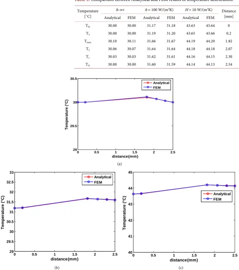
Temperature distribution for analytical calculation and FEM through the com-ponent for each physical situation of the heat-transfer coefficient is presented in
Table 3.
Results of analytical calculation and FEM solution are shown in Figures 7(a)-(c).
Calculation and simulation for h = 0 have not been reported, since tempera-ture are unrealistically high for the multilayer integrated LC component.
[image:7.595.207.540.185.254.2]DOI: 10.4236/eng.2019.1111050 766 Engineering
(a)
(b) (c)
Figure 7. Comparison between analytical and FEM results of temperature distribution: (a) h→∞ , (b) h = 100 W/(m2K), (c) h = 10
W/(m2K).
From these results, it can be observed that for one-dimensional steady state heat conduction problem with uniform heat generation, thermal resistance ap-proach can be used to investigate the temperature distribution inside the multi-layer integrated LC component.
0 0.5 1 1.5 2 2.5
29 29.5 30 30.5
distance(mm)
Tempe
rature (°
C)
Analytical FEM
0 0.5 1 1.5 2 2.5
29 29.5 30 30.5 31 31.5 32 32.5 33
distance(mm)
Tempe
rature (°
C)
Analytical FEM
0 0.5 1 1.5 2 2.5
40 41 42 43 44 45
distance(mm)
Tempe
rature (°
C)
[image:8.595.57.538.78.621.2]DOI: 10.4236/eng.2019.1111050 767 Engineering
5. Conclusion
In this paper, temperature distribution in a multilayer integrated LC has been carried out using conduction and convection heat transfer. Temperature distri-bution in the different material layers has been determined from thermal resis-tance approach knowing the generated heat source and multilayer material properties. Numerical validation of the results of the established model was done using heat transfer module of the FEMM software. A good correlation between analytical calculation using Matlab software and finite element method simula-tion tool for the temperature distribusimula-tion in the integrated LC component has been observed according to the assumptions made.
Acknowledgements
The authors would like to thank Tanoh Aka for his useful discussions.
Conflicts of Interest
The authors declare no conflicts of interest regarding the publication of this pa-per.
References
[1] Hienonen, R., Karjalainen, M. and Lankinen, R. (1997) Verification of the Thermal Design of Electronic Equipment. Technical Research Centre of Finland (VTT). [2] Coulibaly, S., Loum, G. and Diby, K.A. (2015) Design of Integrated LC Filter Using
Multilayer Flexible Ferrite Sheets. IOSR Journal of Electrical and Electronics Engi-neerings (IOSR-JEEE), 10, 35-43.
[3] Coulibaly, S., Loum, G. and Diby, K.A. (2016) Implementation of an Integrated LC Component for the Output Filter of a Step-Down DC-DC Converter. American Scientific Research Journal for Engineering, Technology, and Sciences (ASJETS), 26, 178-189.
[4] Sippola, M. (2003) Developments for the High Frequency Power Transformer De-sign and Implementation. Dissertation for the Degree of Doctor of Science in Tech-nology, Helsinki University of TechTech-nology, Espoo, Finland.
[5] Wolmarans, P.J. (2003) Investigation of a Class of Distributed Planar Conducted RF-EMI Filters for Integration in Power Electronic Converters. Dissertation of Ma-gister Ingeneriae in Electrical and Electronic Engineering, Rand Afrikaans Univer-sity, Johannesburg.
[6] Meeker, D. (2013) Finite Element Method of Magnetics. User’s Manual, Version 4.2.
[7] Pusz, A. and Trojnacki, Z. (2012) The Modeling of Thermal Conductivity Measure-ments Using FEMM Application. Archives of Materials Science and Engineering, 53, 53-60.
[8] Gomadam, P.M., White, R.E. and Weidner, J.W. (2003) Modeling Heat Conduction in Spiral Geometries. Journal of the Electrochemical Society, A1339-A1345.
![Figure 1. Exploded view of the structure [3].](https://thumb-us.123doks.com/thumbv2/123dok_us/8754287.390069/2.595.258.523.495.706/figure-exploded-view-structure.webp)