Word Based Dialog State Tracking with Recurrent Neural Networks

Word-Based Dialog State Tracking

with Recurrent Neural Networks

Matthew Henderson, Blaise Thomson and Steve Young

Department of Engineering, University of Cambridge, U.K.

{mh521, brmt2, sjy}@eng.cam.ac.uk

Abstract

Recently discriminative methods for track-ing the state of a spoken dialog have been shown to outperform traditional generative models. This paper presents a new word-based tracking method which maps di-rectly from the speech recognition results to the dialog state without using an explicit semantic decoder. The method is based on a recurrent neural network structure which is capable of generalising to unseen dialog state hypotheses, and which requires very little feature engineering. The method is evaluated on the second Dialog State Tracking Challenge (DSTC2) corpus and the results demonstrate consistently high performance across all of the metrics.

1 Introduction

While communicating with a user, statistical spo-ken dialog systems must maintain a distribution

over possible dialog states in a process called

di-alog state tracking. This distribution, also called the belief state, directly determines the system’s decisions. In MDP-based systems, only the most likely dialog state is considered and in this case the primary metric is dialog state accuracy (Bo-hus and Rudnicky, 2006). In POMDP-based sys-tems, the full distribution is considered and then the shape of the distribution as measured by an L2 norm is equally important (Young et al., 2009). In both cases, good quality state tracking is essential to maintaining good overall system performance.

Typically, state tracking has assumed the output of a Spoken Language Understanding (SLU) com-ponent in the form of a semantic decoder, which maps the hypotheses from Automatic Speech Recognition (ASR) to a list of semantic hypothe-ses. This paper considers mapping directly from ASR hypotheses to an updated belief state at each

turn in the dialog, omitting the intermediate SLU

processing step. This word-based state tracking

avoids the need for an explicit semantic represen-tation and also avoids the possibility of informa-tion loss at the SLU stage.

Recurrent neural networks (RNNs) provide a natural model for state tracking in dialog, as they are able to model and classify dynamic se-quences with complex behaviours from step to step. Whereas, most previous approaches to dis-criminative state tracking have adapted station-ary classifiers to the temporal process of dialog (Bohus and Rudnicky, 2006; Lee and Eskenazi, 2013; Lee, 2013; Williams, 2013; Henderson et al., 2013b). One notable exception is Ren et al. (2013), which used conditional random fields to model the sequence temporally.

Currently proposed methods of discriminative state tracking require engineering of feature func-tions to represent the turn in the dialog (Ren et al., 2013; Lee and Eskenazi, 2013; Lee, 2013; Williams, 2013; Henderson et al., 2013b). It is un-clear whether differences in performance are due to feature engineering or the underlying models.

This paper proposes a method of using simplen

-gram type features which avoid the need for fea-ture engineering. Instead of using inputs with a se-lect few very informative features, the approach is to use high-dimensional inputs with all the infor-mation to potentially reconstruct any such hand-crafted feature. The impact of significantly in-creasing the dimensionality of the inputs is man-aged by careful initialisation of model parameters. Accuracy on unseen or infrequent slot values is an important concern, particularly for discrim-inative classifiers which are prone to overfitting training data. This is addressed by structuring the recurrent neural network to include a compo-nent which is independent of the actual slot value in question. It thus learns general behaviours for specifying slots enabling it to successfully decode

ASR output which includes previously unseen slot values.

In summary, this paper presents a word-based approach to dialog state tracking using recurrent neural networks. The model is capable of gen-eralising to unseen dialog state hypotheses, and requires very little feature engineering. The ap-proach is evaluated in the second Dialog State Tracking Challenge (DSTC2) (Henderson et al., 2014) where it is shown to be extremely competi-tive, particularly in terms of the quality of its con-fidence scores.

Following a brief outline of DSTC2 in section 2, the definition of the model is given in section 3. Section 4 then gives details on the initialisation methods used for training. Finally results on the DSTC2 evaluation are given in 5.

2 The Second Dialog State Tracking Challenge

This section describes the domain and method-ology of the second Dialog State Tracking Chal-lenge (DSTC2). The chalChal-lenge is based on a large corpus collected using a variety of telephone-based dialog systems in the domain of finding a restaurant in Cambridge. In all cases, the subjects were recruited using Amazon Mechanical Turk.

The data is split into a train, dev and test set. The train and dev sets were supplied with labels, and the test set was released unlabelled for a one week period. At the end of the week, all partici-pants were required to submit their trackers’ out-put on the test set, and the labels were revealed. A mis-match was ensured between training and test-ing conditions by choostest-ing dialogs for the eval-uation collected using a separate dialog manager. This emulates the mis-match a new tracker would encounter if it were actually deployed in an end-to-end system.

In summary, the datasets used are:

• dstc2 train- Labelled training consisting of 1612 dialogs with two dialog managers and two acoustic conditions.

• dstc2 dev - Labelled dataset consisting of 506 calls in the same conditions as dstc2 train, but with no caller in common. • dstc2 test- Evaluation dataset consisting of

1117 dialogs collected using a dialog man-ager not seen in the labelled data.

In contrast with DSTC1, DSTC2 introduces dy-namic user goals, tracking of requested slots and

tracking the restaurant search method. A DSTC2 tracker must therefore report:

• Goals: A distribution over the user’s goal for each slot. This is a distribution over the possi-ble values for that slot, plus the special value

None, which means no valid value has been

mentioned yet.

• Requested slots: A reported probability for each requestable slot that has been requested by the user, and should be informed by the system.

• Method: A distribution over methods, which encodes how the user is trying to use the di-alog system. E.g. ‘by constraints’, when the user is trying to constrain the search, and ‘fin-ished’, when the user wants to end the dialog.

A tracker may report the goals as a joint over all slots, but in this paper the joint is reported as a product of the marginal distributions per slot.

Full details of the challenge are given in Hen-derson et al. (2013a), HenHen-derson et al. (2014). The trackers presented in this paper are identified un-der ‘team4’ in the reported results.

3 Recurrent Neural Network Model This section defines the RNN structure used for dialog state tracking. One such RNN is used per slot, taking the most recent dialog turn (user input plus last machine dialog act) as input, updating its internal memory and calculating an updated belief over the values for the slot. In what follows, the

notationa⊕bis used to denote the concatenation

of two vectors,aandb. Theith_{component of the}

vectorais writtena|i.

3.1 Feature Representation

Extracting n-grams from utterances and dialog

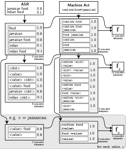
acts provides the feature representations needed for input into the RNN. This process is very sim-ilar to the feature extraction described in Hender-son et al. (2012), and is outlined in figure 1.

For n-gram features extracted from the ASR

N-best list, unigram, bigram and trigram features

are calculated for each hypothesis. These are

then weighted by theN-best list probabilities and

summed to give a single vector.

Dialog acts in this domain consist of a list of component acts of the form

acttype(slot=value) where the slot=value

extracted from each such component act are

‘acttype’, ‘slot’, ‘value’, ‘acttype

slot’, ‘slot value’ and ‘acttype slot

value’, or just‘acttype’for the actacttype().

Each feature is given weight 1, and the features from individual component acts are summed.

To provide a contrast, trackers have also been implemented using the user dialog acts output by an SLU rather than directly from the ASR output.

In this case, the SLUN-best dialog act list is

en-coded in the same way except that the n-grams

from each hypothesis are weighted by the corre-sponding probabilities, and summed to give a sin-gle feature vector.

Consider a word-based tracker which takes an

ASRN-best list and the last machine act as input

for each turn, as shown in figure 1. A combined

feature representation of both the ASRN-best list

and the last machine act is obtained by concate-nating the vectors. This means that in figure 1 the

food feature from the ASR and the food feature

from the machine act contribute to separate

com-ponents of the final vectorf.

f_v ASR food jamaican indian food 1.0 0.9 0.1 <value> food <value> 0.9 0.9 Machine Act confirm food confirm food jamaican food jamaican 1.0 1.0 1.0

e.g. v = jamaican

confirm food <value> food <value>

1.0 1.0

for each value, v jamaican food 0.9

<slot> <value>

1.0 1.0 <value> <slot> 1.0

confirm 1.0 <value> 1.0 confirm <slot> <value> <slot> <value> 1.0 1.0 <value> 1.0 indian 0.1

<value> food 1.0 jamaican <slot> 0.9 indian <slot> 0.1

confirm food <value> 1.0 food <value> 1.0

confirm <slot> jamaican 1.0 <slot> jamaican 1.0 0.9 jamaican food 0.1

indian food confirm(food=jamaican)

food _1.0 <slot> 1.0 f_s f 5 non-zero elements 6 non-zero elements 2 non-zero elements 6 non-zero elements 8 non-zero elements 3 non-zero elements 11 non-zero elements 14 non-zero elements 5 non-zero elements jamaican _1.0

Figure 1: Example of feature extraction for one

turn, givingf,fs andfv. Heres = food. For all

v /∈{indian, jamaican},fv =0.

Note that all the methods for tracking reported in DSTC1 required designing feature functions. For example, suggested feature functions included the SLU score in the current turn, the

probabil-ity of an ‘affirm’ act when the value has been confirmed by the system, the output from base-line trackers etc. (e.g. Lee and Eskenazi (2013), Williams (2013), Henderson et al. (2013b)). In contrast, the approach described here is to present the model with all the information it would need to reconstruct any feature function that might be useful.

3.2 Generalisation to Unseen States

One key issue in applying machine learning to the task of dialog state tracking is being able to deal with states which have not been seen in training. For example, the system should be able to recog-nise any obscure food type which appears in the set of possible food types. A na¨ıve neural

net-work structure mappingn-gram features to an

up-dated distribution for the food slot, with no tying of weights, would require separate examples of

each of the food types to learn whatn-grams are

associated with each. In reality howevern-grams

like‘<value> food’and‘serving<value>’are likely

to correspond to the hypothesis food=‘<value>’for

any food-type replacing‘<value>’.

The approach taken here is to embed a network which learns a generic model of the updated belief of a slot-value assignment as a function of ‘tagged’ features, i.e. features which ignore the specific identity of a value. This can be considered as re-placing all occurrences of a particular value with

a tag like‘<value>’. Figure 1 shows the process of

creating the tagged feature vectors,fsandfv from

the untagged vectorf.

3.3 Model Definition

In this section an RNN is described for tracking

the goal for a given slot, s, throughout the

se-quence of a dialog. The RNN holds an internal

memory, m ∈ RNmem _{which is updated at each}

step. If there areN possible values for slots, then

the probability distribution output p is in RN+1_,

with the last componentp|N giving the

probabil-ity of the Nonehypothesis. Figure 2 provides an

overview of howpandmare updated in one turn

to give the new belief and memory,p0_andm0_.

One part of the neural network is used to learn a mapping from the untagged inputs, full memory

and previous beliefs to a vector h ∈ RN _which

goes directly into the calculation ofp0_:

p m

h

N. Net.

gv pv

N. Net. for each value, v

h+g

p’

softmax m

’

logistic for each slot, s f

f_s

fv

pN

Figure 2: Calculation ofp0_andm0_{for one turn}

where NNet(·) denotes a neural network function

of the input. In this paper all such networks have one hidden layer with a sigmoidal activation func-tion.

The sub-network forhrequires examples of

ev-ery value in training, and is prone to poor general-isation as explained in section 3.2. By including a

second sub-network forgwhich takes tagged

fea-tures as input, it is possible to exploit the obser-vation that the string corresponding to a value in various contexts is likely to be good evidence for

or against that value. For each valuev, a

compo-nent ofgis calculated using the neural network:

g|v = NNet

f⊕fs⊕fv⊕

{p|v, p|N} ⊕m

∈R

By using regularisation, the learning will

pre-fer where possible to use the sub-network for g

rather than learning the individual weights for

each value required in the sub-network forh. This

sub-network is able to deal with unseen or infre-quently seen dialog states, so long as the state can be tagged in the feature extraction. This model can

also be shared across slots sincefsis included as

an input, see section 4.2.

The sub-networks applied to tagged and un-tagged inputs are combined to give the new belief:

p0 _{= softmax ([h+g]⊕ {B})∈R}N+1

whereB is a parameter of the RNN, contributing

to theNonehypothesis. The contribution fromg

may be seen as accounting for general behaviour

of tagged hypotheses, whileh makes corrections

due to correlations with untagged features and

value specific behaviour e.g. special ways of ex-pressing specific goals and fitting to specific ASR confusions.

Finally, the memory is updated according to the logistic regression:

m0 _{= σ(W}

m0f+Wm1m)∈RNmem

where theWmiare parameters of the RNN.

3.4 Requested Slots and Method

A similar RNN is used to track the requested slots.

Here thevruns over all the requestable slots, and

requestable slot names are tagged in the feature

vectorsfv. This allows the neural network

calcu-latingg to learn general patterns across slots just

as in the case of goals. The equation for p0 _is

changed to:

p0 _{= σ(h+g)}

so each component ofp0_{represents the probability}

(between 0 and 1) of a slot being requested. For method classification, the same RNN struc-ture as for a goal is used. No tagging of the feastruc-ture vectors is used in the case of methods.

4 Training

The RNNs are trained using Stochastic Gradient Descent (SGD), maximizing the log probability of the sequences of observed beliefs in the training data (Bottou, 1991). Gradient clipping is used to avoid the problem of exploding gradients (Pascanu et al., 2012). A regularisation term is included,

which penalises thel2 norm of all the parameters.

It is found empirically to be beneficial to give more weight in the regularisation to the parameters used

in the network calculatingh.

When using the ASR N-best list, f is

typi-cally of dimensionality around 3500. With so many weights to learn, it is important to initialise the parameters well before starting the SGD algo-rithm. Two initialisation techniques have been in-vestigated, the denoising autoencoder and shared initialisation. These were evaluated by training trackers on the dstc2 train set, and evaluating on dstc2 dev (see table 1).

4.1 Denoising Autoencoder

Joint Goals Method Requested Shared

init. dAinit. Acc L2 Acc L2 Acc L2

0.686 0.477 0.913 0.147 0.963 0.059 X 0.688 0.466 0.915 0.144 0.962 0.059 X 0.680 0.479 0.910 0.152 0.962 0.059

X X 0.696 0.463 0.915 0.144 0.965 0.057

Baseline: 0.612 0.632 0.830 0.266 0.894 0.174

Table 1: Performance on the dev set when varying initialisation techniques for word-based tracking. Acc

denotes the accuracy of the most likely belief at each turn, and L2 denotes the squaredl2 norm between

the estimated belief distribution and correct (delta) distribution. For each row, 5 trackers are trained

and then combined using score averaging. The final row shows the results for thefocus-based baseline

tracker (Henderson et al., 2014).

underlying representations of the input, has been found effective as an initialisation technique in deep learning (Vincent et al., 2008).

A dA is used to initialise the parameters of the RNN which multiply the high-dimensional input

vectorf. The dA learns a matrixWdAwhich

re-duces f to a lower dimensional vector such that

the original vector may be recovered with minimal loss in the presence of noise.

For learning the dA,f is first mapped such that

feature values lie between 0 and 1. The dA takes as

inputfnoisy, a noisy copy off where each

compo-nent is set to 0 with probabilityp. This is mapped

to a lower dimensional hidden representationh:

h=σ(WdAfnoisy+b0)

A reconstructed vector, frec, is then calculated

as:

frec=σ WdAT h+b1

The cross-entropy betweenf andfrecis used as

the objective function in gradient descent, with an

addedl1regularisation term to ensure the learning

of sparse weights. As the ASR features are likely to be very noisy, dense weights would be prone to

overfitting the examples.1

When using WdA to initialise weights in the

RNN, training is observed to converge faster. Ta-ble 1 shows that dA initialisation leads to better solutions, particularly for tracking the goals.

4.2 Shared Initialisation

It is possible to train a slot-independent RNN,

us-ing trainus-ing data from all slots, by not includus-ingh

in the model (the dimensionality ofhis dependent

1_{The state-of-the-art in dialog act classification with very}

similar data also uses sparse weights Chen et al. (2013).

on the slot). Inshared initialisation, such an RNN

is trained for a few epochs, then the learnt param-eters are used to initialise slot-dependent RNNs for each slot. This follows the shared initialisation procedure presented in Henderson et al. (2013b).

Table 1 suggests that shared initialisation when combined with dA initialisation gives the best per-formance.

4.3 Model Combination

In DSTC1, the most competitive results were achieved with model combination whereby the output of multiple trackers were combined to give more accurate classifications (Lee and Eskenazi, 2013). The technique for model combination used here is score averaging, where the final score for each component of the dialog state is computed as the mean of the scores output by all the trackers being combined. This is one of the simplest meth-ods for model combination, and requires no extra training data. It is guaranteed to improve the accu-racy if the outputs from the individual trackers are not correlated, and the individual trackers operate

at an accuracy>0.5.

Multiple runs of training the RNNs were found to give results with high variability and model combination provides a method to exploit this variability. In order to demonstrate the effect, 10 trackers with varying regularisation parame-ters were trained on dstc2 train and used to track dstc2 dev. Figure 3 shows the effects of combin-ing these trackers in larger groups. The mean

ac-curacy in the joint goals from combiningm

track-ers is found to increase withm. The single output

from combining all 10 trackers outperforms any single tracker in the group.

vary-A

ccuracy

# trackers combined, m

1 2 3 4 5 6 7 8 9 10

0.64 0.65 0.66 0.67 0.68 0.69 0.70 0.71 0.72

Figure 3: Joint goal accuracy on dstc2 dev from system

combination. Ten total trackers are trained with varying reg-ularisation parameters. For eachm = 1. . .10, all subsets of sizemof the 10 trackers are used to generate10_Cm com-bined results, which are plotted as a boxplot. Boxplots show minimum, maximum, the interquartile range and the median. The mean values are plotted as connected points.

ing model hyper-parameters (e.g. regularisation parameters, memory size) and combine their out-put using score averaging. Note that maintaining around 10 RNNs for each dialog state components is entirely feasible for a realtime system, as the RNN operations are quick to compute. An un-optimised Python implementation of the tracker including an RNN for each dialog state compo-nent is able to do state tracking at a rate of around 50 turns per second on an Intel® Core™ i7-970 3.2GHz processor.

5 Results

The strict blind evaluation procedure defined for the DSTC2 challenge was used to investigate the effect on performance of two contrasts. The first contrast compares word-based tracking and con-ventional tracking based on SLU output. The sec-ond contrast investigates the effect of including

and omitting the sub-network forh in the RNN.

Recallhis the part of the model that allows

learn-ing special behaviours for particular dialog state hypotheses, and correlations with untagged fea-tures. These two binary contrasts resulted in a to-tal of 4 system variants being entered in the chal-lenge.

Each system is the score-averaged combined output of 12 trackers trained with varying hyper-parameters (see section 4.3). The performance of the 4 entries on the featured metrics of the chal-lenge are shown in table 2.

It should be noted that the live SLU used the word confusion network, not made available in the challenge. The word confusion network is known

to provide stronger features than theN-best list for

language understanding (Henderson et al., 2012; T¨ur et al., 2013), so the word-based trackers

us-ing N-best ASR features were at a disadvantage

in that regard. Nevertheless, despite this hand-icap, the best results were obtained from word-based tracking directly on the ASR output, rather than using the confusion network generated SLU

output. Includingh always helps, though this is

far more pronounced for the word-based

track-ers. Note that trackers which do not includehare

value-independent and so are capable of handling new values at runtime.

The RNN trackers performed very competi-tively in the context of the challenge. Figure 4 vi-sualises the performance of the four trackers rela-tive to all the entries submitted to the challenge for the featured metrics. For full details of the evalua-tion metrics see Henderson et al. (2014). The box in this figure gives the entry IDs under which the results are reported in the DSTC (under the team ID ‘team4’). The word-based tracker including

h(h-ASR), was top for joint goals L2 as well as

requested slots accuracy and L2. It was close to the top for the other featured metrics, following closely entries from team 2. The RNN trackers performed particularly well on measures assessing the quality of the scores such as L2.

There are hundreds of numbers reported in the

DSTC2 evaluation, and it was found that the h

-ASR tracker ranked top on many of them. Consid-ering L2, accuracy, average probability, equal er-ror rate, log probability and mean reciprocal rank across all components of the the dialog state, these

give a total of 318 metrics. The h-ASR tracker

ranked top of all trackers in the challenge in 89 of these metrics, more than any other tracker. The

ASR tracker omittinghcame second, ranking top

in 33 of these metrics.

The trackers using SLU features ranked top in all of the featured metrics among the trackers which used only the SLU output.

6 Conclusions

Tracker

Inputs Joint Goals Method Requested

entry Include_h Live_ASR Live_SLU Acc L2 ROC Acc L2 ROC Acc L2 ROC

0 X X 0.768 0.346 0.365 0.940 0.095 0.452 0.978 0.035 0.525

1 X 0.746 0.381 0.383 0.939 0.097 0.423 0.977 0.038 0.490

2 X X 0.742 0.387 0.345 0.922 0.124 0.447 0.957 0.069 0.340

3 X 0.737 0.406 0.321 0.922 0.125 0.406 0.957 0.073 0.385

Table 2: Featured metrics on the test set for the 4 RNN trackers entered to the challenge.

0.4 1.0

0.6 0.8

0.0 0.8

A

ccuracy

Joint Goals Method Requested All

0.2 0.4 0.6

L2

entry0 entry2

entry1 entry3

word-based

SLU input

full model no h

baseline

Figure 4: Relative performance of RNN trackers for

fea-tured metrics in DSTC2. Each dash is one of the 34 trackers evaluated in the challenge. Note a lower L2 is better. ROC metric is only comparable for systems of similar accuracies, so is not plotted. Thefocusbaseline system is shown as a circle.

lost in the omitted SLU step.

In general, the RNN appears to be a promising model, which deals naturally with sequential input and outputs. High dimensional inputs are handled well, with little feature engineering, particularly when carefully initialised (e.g. as here using de-noising autoencoders and shared initialisation).

Future work should include making joint pre-dictions on components of the dialog state. In this paper each component was tracked using its own RNN. Though not presented in this paper, no im-provement could be found by joining the RNNs. However, this may not be the case for other do-mains in which slot values are more highly cor-related. The concept of tagging the feature func-tions allows for generalisation to unseen values and slots. This generalisation will be explored in future work, particularly for dialogs in more open-domains.

Acknowledgements

Matthew Henderson is a Google Doctoral Fellow.

References

Dan Bohus and Alex Rudnicky. 2006. A

K-hypotheses+ Other Belief Updating Model. Proc. of the AAAI Workshop on Statistical and Empirical Methods in Spoken Dialogue Systems.

L´eon Bottou. 1991. Stochastic gradient learning in neural networks. In Proceedings of Neuro-Nˆımes 91, Nˆımes, France. EC2.

Yun-Nung Chen, William Yang Wang, and Alexan-der I Rudnicky. 2013. An empirical investigation of sparse log-linear models for improved dialogue act classification. InAcoustics, Speech and Signal Pro-cessing (ICASSP), 2013 IEEE International Confer-ence on.

Matthew Henderson, Blaise Thomson, and Jason Williams. 2013a. Dialog State Tracking Challenge 2 & 3 Handbook. _{camdial.org/˜mh521/dstc/}. Matthew Henderson, Blaise Thomson, and Steve

Young. 2013b. Deep Neural Network Approach for the Dialog State Tracking Challenge. In Proceed-ings of SIGdial, Metz, France, August.

Matthew Henderson, Blaise Thomson, and Jason Williams. 2014. The second dialog state tracking challenge. InProceedings of the SIGdial 2014 Con-ference, Baltimore, U.S.A., June.

Sungjin Lee and Maxine Eskenazi. 2013. Recipe for building robust spoken dialog state trackers: Dialog state tracking challenge system description. In Pro-ceedings of the SIGDIAL 2013 Conference, Metz, France, August.

Sungjin Lee. 2013. Structured discriminative model for dialog state tracking. InProceedings of the SIG-DIAL 2013 Conference, Metz, France, August. Razvan Pascanu, Tomas Mikolov, and Yoshua Bengio.

2012. Understanding the exploding gradient prob-lem. CoRR.

Hang Ren, Weiqun Xu, Yan Zhang, and Yonghong Yan. 2013. Dialog state tracking using conditional ran-dom fields. In Proceedings of the SIGDIAL 2013 Conference, Metz, France, August.

G¨okhan T¨ur, Anoop Deoras, and Dilek Hakkani-T¨ur. 2013. Semantic parsing using word confusion net-works with conditional random fields. In INTER-SPEECH.

Pascal Vincent, Hugo Larochelle, Yoshua Bengio, and Pierre-Antoine Manzagol. 2008. Extracting and composing robust features with denoising autoen-coders. In Proceedings of the 25th International Conference on Machine Learning, Helsinki, Fin-land.

Jason Williams. 2013. Multi-domain learning and gen-eralization in dialog state tracking. InProceedings of the SIGDIAL 2013 Conference, Metz, France, Au-gust.