Effect of small sample size on text categorization with support vector
machines
Paweł Matykiewicz
Biomedical Informatics Cincinnati Children’s Hospital
3333 Burnet Ave Cincinnat, OH 45220, USA
John Pestian
Biomedical Informatics Cincinnati Children’s Hospital
3333 Burnet Ave Cincinnat, OH 45220, USA
Abstract
Datasets that answer difficult clinical ques-tions are expensive in part due to the need for medical expertise and patient informed con-sent. We investigate the effect of small sample size on the performance of a text categoriza-tion algorithm. We show how to determine whether the dataset is large enough to train support vector machines. Since it is not pos-sible to cover all aspects of sample size cal-culation in one manuscript, we focus on how certain types of data relate to certain proper-ties of support vector machines. We show that normal vectors of decision hyperplanes can be used for assessing reliability and internal cross-validation can be used for assessing sta-bility of small sample data.
1 Introduction
Every patient visit generates data, some on paper, some stored in databases as structured form fields, some as free text. Regardless of how they are stored, all such data are to be used strictly for pa-tient care and for billing, not for research. Papa-tient health records are maintained securely according to the provisions of the Health Insurance Portability and Accountability Act (HIPAA). Investigators must obtain informed consent from patients whose data will be used for other purposes. This means defin-ing which data will be used and how they will be used. In addition to writing protocols and obtain-ing consent from patients, medical experts must ei-ther manually codify important information or teach a machine how to do it. All of these labor-intensive
tasks are expensive. No one wants to collect more data than is necessary.
Our research focuses on answering difficult neu-ropsychiatric questions such as, “Who is at higher risk of dying by suicide?” or “Who is a good candidate for epilepsy surgery evaluation?” Large amounts of data that might answer these questions exist in the form of text dictated by clinicians or written by patients and thus unavailable. Parallel to the collection of such data, we explored whether small datasets can be used to build reliable methods of making this information available. Here, we in-vestigate how text classification training size relates to certain aspects of linear support vector machines. We hypothesize thata sufficiently large training sub-set will generate stable and reliable performance es-timates of a classifier. On the other hand, if the dataset is too small, then even small changes to the training size will change the performance of a classifier and manifest unstable and unreliable esti-mates. We introduce quantitive definitions for sta-bility and reliasta-bility and give empirical evidence on how they work.
2 Background
How much data is needed for reliable and stable analysis? This question has been answered for most univariate problems, and a few solutions exist for multivariate problems, but no widely accepted an-swer is available for sparse and high-dimensional data. Nonetheless, we will review the few sample size calculation methods that have been used for ma-chine learning.
Hsieh et al. (1998) described a method for calcu-lating the sample size needed for logistic and lin-ear regression models. The multivariate problem was simplified to a series of univariate two-sample t-tests on the input variables. A variance inflation fac-tor was used to correct for the multi-dimensionality which quantifies the severity of multicollinearity in the least squares regression: collinearity deflates and non-collinearity inflates sample size estima-tion. Computer simulations were done on low-dimensional and continuous data, so it is not known whether the method is applicable to text categoriza-tion.
Guyon et al. (1998) addressed the problem of de-termining what size test set guarantees statistically significant results in a character recognition task, as a function of the expected error rate. This method does not assume which learner will be used. Instead, it requires specific parameters that describe hand-writing data collection properties such as between-writers variance and within-writer variance. The downside of this method is that it must assume the worst-case scenario: a large variance in data and a low error rate for the classifier. For this reason larger datasets are recommended.
Dobbin et al. (2008) and Jianhua Hu (2005) fo-cused only on sample size for a classifier that learns from gene expression data. No assumptions were made about the classifier, only about the data struc-ture. All gene expressions were measured on a con-tinuous scale that denotes some luminescence cor-responding to the relative abundance of nucleic acid sequences in the target DNA strand. The data, re-gardless of size, can be qualified using just one pa-rameter, fold change, which measures changes in the expression level of a gene under two different con-ditions. Furthermore, the fold change can be stan-dardized for compatibility with other biological ex-periments: with a lower standardized fold change, more samples are needed, and with more genes, more samples are needed. There is a strong assump-tion about data makeup, but no assumpassump-tion is made about the classifier. This solution allows for small sample sizes but does not generalize to text classifi-cation data.
Way et al. (2010) evaluated the performance of various classifiers and featured a selection technique in the presence of different training sample sizes.
Experiments were conducted on synthetic data, with two classes drawn from multivariate Gaussian dis-tributions with unequal means and either equal or unequal covariance matrices. The conclusion was that support vector machines with a radial kernel performed slightly better than the LDA when the training sample size was small. Only certain combi-nations of feature selection and classification meth-ods work well with small sample sizes. We will use similar assumptions for sparse and high-dimensional data.
Most recently, Juckett (2012) developed a method for determining the number of documents needed for a gold standard corpus. The sample size calculation was based on the concept of capture probabilities. It is defined as the normalized sum of probabilities over all words of interest. For example, if the re-quired capture probability is 0.95 for a set of med-ical words, when using larger corpora that contain these words, it must first be calculated how many documents are needed to capture the same probabil-ity in the target corpus. This method is specific to linguistic research on annotated corpora, where the probabilities of individual words in the sought cor-pora must match the probabilities of words in the target domain. This method focuses solely on the data structure and does not assume an algorithm or the task that it will serve. The downside is a higher sample size.
When reviewing various methods for sample size calculation, we found that as more assumptions can be made, fewer data are needed for meaningful anal-ysis. Assumptions can be made about data structure and quality, the task the data serve, feature selection, and the classifier. Our approach exploits a scenario where the task, the feature selection, and the classi-fier are known.
3 Data
The first dataset was created by Anderson (1935) and introduced to the world of statistics by Fisher (1936). Since then it has been used on countless oc-casions to benchmark machine learning algorithms. Each row of data has four variables to describe the shape of an iris calyx: sepal length, sepal width, petal length, and petal width. The dataset contains 50 measurements for each of three subspecies of the iris flower: setosa, versicolor, and virginica. All measurements of the setosa calyx are separable from the rest of the data and thus were not used in our ex-periments. Instead, we used data corresponding to versicolor and virginica (VV), which is more inter-esting because of a small class overlap. The noise is introduced mostly by sepal width and sepal length.
The second dataset was created by Lewis and Ringuette (1994) and is the one most commonly used to benchmark text classification algorithms. The collection is composed of 21,578 short news stories from the Reuters news agency. Some stories have manually assigned topics, like “earn,” “acq,” or “money-fx,” and others do not. In order to make the dataset comparable across different uses, a “Modi-fied Apte” (“ModApte”) split was proposed by Apt´e et al. (1994). It has 9,603 training and 3,299 exter-nal testing documents, a total of 135 distinct topics, with at least one topic per document. The most fre-quent topic is “earn,” which appears in 3,964 docu-ments. Here, we used only the “wheat” and “corn” categories, which appear 212 and 181 times in the training set along with 71 and 56 cases in the test set. These topics are semantically related, so it is no surprise that 59 documents in the training set and 22 documents in test set have both labels. This gives a total of 335 unique training instances and 105 unique test instances. Interestingly, it is eas-ier to distinguish “corn” news from “not corn just wheat” news than it is to distinguish “wheat” from “not wheat just corn.” The latter seems to be a good dataset for benchmarking sample size calculation. We will refer to the “wheat” versus “not wheat” training set as WCT and the “wheat” versus “not wheat” external test set asWCE.
The third dataset was extracted from the appendix in Shneidman and Farberow (1957). It contains 66 suicide notes (SN) organized into two categories: 33 genuine and 33 simulated. The authors of the notes were matched in both groups by gender (male), race
(white), religion (Protestant), nationality (native-born U.S. citizens), and age (25-59). Authors of the simulated suicide notes were screened for personal-ity disorders or tendencies toward morbid thoughts that would exclude them from the study. Individu-als enrolled in the study were asked to write a sui-cide note as if they were going to take their own life. Notes were anonymized, digitized, and prepared for text processing (Pestian et al., 2010).
The fourth dataset was collected in a clinical con-trolled trial at Cincinnati Children’s Hospital Med-ical Center Emergency Department. Sixty patients were enrolled, 30 with suicidal behavior and 30 con-trols from the orthopedic service. The suicidal be-havior group comprised 15 females and 15 males with an average age of≈15.7 years (SD ≈1.15). The control group included 15 females and 15 males with an average age of≈14.3 years (SD ≈1.21). The interview consisted of five open-ended ubiqui-tous questions (UQ): “Does it hurt emotionally?” “Do you have any fear?” “Are you angry?” “Do you have any secrets?” and “Do you have hope?” The interviews were recorded in an audio format, transcribed by a medical transcriptionist, and pre-pared for analysis by removing the sections of the interview where the questions were asked. To pre-serve the UQ structure, n-grams from each of the five questions were separated (Pestian et al., 2012).
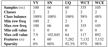
VV SN UQ WCT WCE
Samples(m) 100 66 60 335 105
Classes 2 2 2 2 2
Class balance 100% 100% 100% 58% 48%
Min row freq 100 2 2 3 0
Max row freq 100 66 60 335 105
Min cell value 1 0 0 0 0
Max cell value 7.9 102.045 64 117 892
Features(n) 4 60 7,282 7,132 7,132
[image:3.612.315.538.462.560.2]Sparsity 0% 60% 92.3% 97% 98%
4 Methods
Feature extraction. Every text classification algo-rithm starts with feature engineering. Documents in theUQ,WCT, andWCEsets were represented by a bag-of-n-grams model (Manning and Schuetze, 1999; Manning et al., 2008). Every document was tokenized, and frequencies of unigrams, bigrams, and trigrams were calculated. All digit numbers that appeared in a document were converted to the same token (”NUMB”). Documents become row vectors and n-grams become column vectors in a large sparse matrix. Each n-gram has its own dimen-sion, with the exception ofUQdata, where n-grams are represented separately for each of the five ques-tions. Neither stemming nor a stop word list were applied to the textual data. Suicide notes (SN) were not represented by n-grams. In previous studies, we found that the structure of the note and its emotional content are indicative of suicidality, not its seman-tic content. Hence, the SN dataset is represented by the frequency of 23 emotions assigned by men-tal health professionals, the frequency of 34 parts of speech, and by three readability scores: Flesch, Fog, and Kincaid.
Feature weighting. Term weighting was chosen
ad hoc. UQ, WCT, and WCE had a logarithmic term frequency (log-tf) as local weighting and an in-verse document frequency (idf) as global weighting but were derived only from the training data (Salton and Buckley, 1988; Nakov et al., 2001).
Feature selection. To speed up calculations, the least frequent features were removed from theSN, UQ,WCT, and WCE datasets (see minimum row frequency in Table 1). Further optimization of the feature space was done using an information gain filter (Guyon and Elisseeff, 2003; Yang and Peder-sen, 1997). Depending on the experiment, some of the features with the lowest information gain were removed. For example,IG = 0.4 means that 40% of the features, those with a higher information gain, were kept, and the other 60%, those with a lower in-formation gain, were removed. Lastly, all row vec-tors in UQ, WCT, and WCE were normalized to unit length (Joachims, 1998).
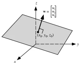
[image:4.612.360.488.55.157.2]Learning algorithm.We used linear support vec-tor machines (SVM) to learn from the data. Sup-port vector machines are described in great detail in
Figure 1: Normal vectorwof a hyperplane.
Schlkopf and Smola (2001). We will focus on just two aspects: properties of the normal vector of de-cision hyperplane (see Figure 1) and internal cross-validation (see Figure 2). SVMis in essence a sim-ple linear classifier:
f(x) = sgn(hw,xi+b) (1)
wherexis an input vector that needs to be classified,
h·,·iis the inner product, wis a weight vector with the same dimensionality asx, andbis a scalar. The functionf outputs+1ifxbelongs to the first class or−1ifxbelongs to the second class.SVMdiffers from other linear classifiers on howwis computed. Contrary to other classifiers, it does not solvew di-rectly. Instead, it uses convex optimization to find vectors from the training set that can be used for cre-ating the largest margin between training examples from the first and second class. Hence, the solution towis in the form of the linear combination of co-efficients and training vectors:
w=
m X
i=1
αiyixi (2)
wheremis the number of training vectors,αi ≥ 0
are Lagrange multipliers, yi ∈ {−1,1} are
numer-ical codes for class labels, andxi are training row
vectors. Vectorw is perpendicular to the decision boundary, and its proper name in the context of SVM is the normal vector of decision hyperplane1 (see Figure 1). One of the properties ofSVMis that outlying training vectors are not used inw. These vectors have the corresponding coefficientαi = 0.
In fact, these vectors can be removed from the train-ing set and the convex optimization procedure will
1If
result in exactly the same solution. We can use this property to probe how reliable training data are for the classification task. If we have enough data that we can randomly remove some, what is left will re-sult in w∗ ≈ w. On the other hand, if we do not have enough data, then random removal of training data will result in a very different equation, because the decision boundary changes andw∗ 6=w.
Reliability of performance.The relationship be-tweenw∗andwcan be measured. We introduce the SVMreliability index (SRI):
SRI(w∗,w) =|r(w∗,w)| (3)
= |
Pn
i=1(wi∗−w∗)(wi−w)| pPn
i=1(w∗i −w∗)2 pPn
i=1(wi−w)2
which is the absolute value of the Pearson product-moment correlation coefficient between convex op-timization solution w∗ corresponding to a training subset and w corresponding to the full dataset2. Pearson’s correlation coefficient discovers linear de-pendency between two normally distributed random variables and has its domain on a continuous seg-ment between −1 and +1. In our case, we are looking for a strong linear dependency between con-stituents of the training weight vectorw∗i and con-stituents of the full dataset weight vectorwi. Some
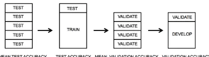
numerical implementations of SVM cause the out-put values for the class labels to switch. We cor-rected for this effect by applying absolute value to the Pearson’s coefficient, resulting inSRI ∈ [0,1]. We did not have a formal proof on howSRIrelates to SVM performance. Instead, we showed empir-ical evidence for the relationship based on a few small benchmark data. Stability of performance. SVM generalization performance is usually mea-sured using cross-validation accuracy. In particu-lar, we use balanced accuracy because it gives bet-ter evidence for a drop in performance when solving unbalanced problems. Following Guyon and Elis-seeff (2003) and many others, we divided the data into three sets: test, training, and validation. Mean test balanced accuracyaT is estimated using strati-fied Monte Carlo cross-validation (MCCV), where
2
[image:5.612.321.529.59.116.2]We experimented with Pearson’s correlation, Spearman’s correlation, one-way intraclass correlation, Cosine correlation, Cronbach’s coefficient, and Krippendorff’s coefficients and found that Pearson’s correlation coefficient works well with both low-dimensional and high-dimensional spaces.
Figure 2: Estimation and resampling: mean test balanced accuracy and mean validation balanced accuracy should match. To prevent overfitting, tuning machine learning should be guided by mean validation accuracy and con-firmed by mean test accuracy. This procedure requires the “develop” set to be large enough to give reliable and stable estimates.
the proportion of the training set to the test set is varied between 0.06 and 0.99. Mean validation bal-anced accuracy aV (MVA) is estimated using K -fold validation (also known as internal cross-validation), where K = m2 and m is the number of training cases. In the case of the “wheat” versus “not wheat just corn” dataset, we have, in addition, the external validation setWCEand corresponding mean external balanced accuracyaE. Correct esti-mation of the learner’s generalization performance should result in all three accuracies being equal:
aT ≈aV ≈aE. Furthermore, we want all three ac-curacies to be the same regardless of the amount of data. If we have enough data that we can randomly remove some, what is left will result inaV∗ ≈aV∗∗. On the other hand, if we do not have enough data, then random removal of training data will result in very different accuracy estimations:aV∗ 6=aV∗∗.
Sample size calculation. We do not have a good way of predicting how much data will be needed to solve a problem with a small p-value, but this is a matter of convenience. Rather than looking to the future, we can simply ask if what we have now is enough. If we can build a classifier that gives re-liable and stable estimates of performance, we can stop collecting data. Reliability is measured bySRI, while stability is measured byMVA, not as a single value but merely as a function of the training size:
SRI(t) =|r(wtm,wm)| and (4)
aT(t) =aTtm (5)
where t is a proportion of the training data, t ∈
ability of the dataset to produce classification mod-els with reliable and stable performance estimates, we need two more measures: sample dispersion of SRIand sample dispersion ofMVA:
cSRI(t≥p) =
sSRI(t≥p)
SRI(t≥p) and (6)
cM V A(t≥p) =
saT(t≥p)
aT(t≥p) (7)
defined as the coefficient of variation of allSRI or MVA measurements for training data sizes greater thanpm˙. For example, we want to know if our 10-fold cross-validation (CV) for a dataset that has 400 training samples is reliable and stable. 10-fold CV is 0.9 of training data, so we need to measureSRI andMVAfor different proportions of training data,
t = {0.90,0.91, . . . ,0.99}, and then calculate dis-persion forcSRI(t≥0.9)andcM V A(t≥0.9).
Nu-merical calculations will give us sense of good and bad dispersion across different datasets.
5 Results
Do I have enough data? The first set of experi-ments was done with untuned algorithms. We set the SVMparameter toC = 1and did not use any fea-ture selection. Figure 3 shows four examples of how SVMperformance depends on the training set size. The performance was measured using mean test bal-anced accuracy, MVA, and SRI. Numerical calcu-lations showed thatVVneeds at least 30 randomly selected training examples to produce reliable and stable results with high accuracy. cSRI(t ≥ 0.75)
is 0.005 and cM V A(t ≥ 0.75) is 0.016. SN was
not encouraging regarding the estimated accuracy; SRIdropped, suggesting that theSVMdecision hy-perplanes are unreliable. Mental health profession-als can distinguish between genuine and simulated notes about 63% of time. Machine learning does it correctly about 73% of time if text structure and emotional content are used. Even so, the sample size calculation yields high dispersion (cSRI(t ≥
0.75) = 0.134 and cM V A(t ≥ 0.75) = 0.082).
UQis small and high-dimensional, and yet the re-sults were reliable and stable (cSRI(t ≥ 0.75) =
0.015 and cM V A(t ≥ 0.75) = 0.023). Patients
enrolled in the UQ study also received the Sui-cide Ideation Questionnaire (Raynolds, 1987) and
the Columbia-Suicide Severity Rating Scale (Pos-ner et al., 2011). We found that UQ was no dif-ferent from the structured questionnaires. UQ de-tects suicidality mostly by emotional pain and hope-lessness, which were mildly present in four control patients. Other instruments returned errors because the same few teenagers reported risky behavior and morbid thoughts. WCT produced reliable and sta-ble accuracy estimates, but no large amounts of data could be removed (cSRI(t ≥ 0.75) = 0.010and
cM V A(t ≥ 0.75) = 0.053). It seems that WCE
is somehow different from WCT, or it might be a case of overfitting, which causes the mean test ac-curacy to diverge fromMVAas the training dataset gets smaller. Algorithm tuning. No results should be regarded as satisfactory until a thorough param-eter space search has been completed. Each step of a text classification algorithm can be improved. To attempt a complete description of the dependency of a minimal viable sample size on text classifica-tion would be both impossible and futile, since new methods are discovered every day. However, to start somewhere, we focused only on the feature selection andSVMparameterC3. Feature selection removes noise from data. Parameter C informs the convex optimization process about the expected noise level. If both parameters are set correctly, we should see an improvement in the reliability and stability of the results. There are several methods for tuning SVM; the most commonly used but computation-ally expensive is internal cross-validation (Duan et al., 2003; Chapelle et al., 2002). Figure 5 shows the results of the parameter tuning procedure. VV andSNare not extremely high-dimensional, so we tuned just parameterC. MVAmaxima were found atC = 0.45withVV,C = 0.05withSN,C = 0.4 and IG = 0.1584 with UQ, and C = 2.5 and
IG = 0.8020withWCT. Do I have enough data after algorithm tuning? Internal cross-validation (MVA) did not improve dispersion universally (see Table 2). VVimproved on reliability but not stabil-ity. SN scored much better on both measures, but we do not yet know what the cutoff for having a low enough dispersion is.UQdid worse on all mea-sures after tuning. WCTimproved greatly on mean
3
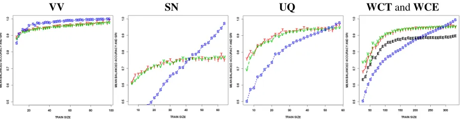
VV SN UQ WCTandWCE
Figure 3: SRIindex (S),MVAaccuracy (V) and mean test accuracy (T) averaged over 120 repetitions and different training data sizes. LinearSVMwithC= 1and no feature selection. VV(cSRI(t ≥0.75) = 0.005andcM V A(t≥
0.75) = 0.016),UQ(cSRI(t≥0.75) = 0.015andcM V A(t≥0.75) = 0.023), andWCT(cSRI(t≥0.75) = 0.010
andcM V A(t ≥ 0.75) = 0.053) gave stable and reliable estimates, butSNdid not (cSRI(t ≥ 0.75) = 0.134and
cM V A(t≥0.75) = 0.082).
[image:7.612.75.535.295.415.2]VV SN UQ WCT
Figure 4: MVA (internal cross-validation) parameter tuning results. Maxima were found atC = 0.45 withVV,
C= 0.05withSN,C= 0.4andIG= 0.1584withUQ, andC= 2.5andIG= 0.8020withWCT.
VV SN UQ WCTandWCE
Figure 5: SRIindex (S),MVAaccuracy (V), and mean test accuracy (T) averaged over 60 repetitions and different training data sizes. Tuned classification algorithms: VVwithC = 0.45and no feature selection,SNwithC = 0.05
and no feature selection,UQwithC= 0.4andIG= 0.1584, andWCTwithC = 2.5andIG = 0.8020. Stability and reliability: VVhadcSRI(t≥0.75) = 0.003andcM V A(t≥0.75) = 0.018),SNhadcSRI(t ≥0.75) = 0.085
andcM V A(t ≥ 0.75) = 0.075,UQ hadcSRI(t ≥ 0.75) = 0.025andcM V A(t ≥ 0.75) = 0.024, andWCThad
[image:7.612.73.536.485.607.2]test accuracy, mean external validation, and stability dispersion (see Figure 5). It would be interesting to see if improvement on both reliability dispersion and stability dispersion would bring mean test accuracy and mean external validation even closer together.
aT(t≥0.75)c
SRI(t≥0.75)cM V A(t≥0.75) VVno tuning 0.965 0.005 0.016
SNno tuning 0.744 0.134 0.082
UQno tuning 0.946 0.015 0.023 WCTno tuning 0.862 0.010 0.053
VVwith tuning 0.970 0.003 0.018
SNwith tuning 0.755 0.085 0.075 UQwith tuning 0.941 0.025 0.024
WCTwith tuning0.946 0.025 0.011
Table 2: Sample size calculation before and after tuning with internal cross-validation (MVA). Even though mean test accuracy (aT(t≥0.75)) improved forVV,SN, and WCT, reliability and stability did not improve univer-sally. Internal cross-validation alone might not be ade-quate for tuning classification algorithms for all data.
6 Discussion
Sample size calculation data for a competition and for problem-solving.In general, there might be two conflicting objectives when calculating whether what we have collected is a large enough dataset. If the objective is to have a shared task with many par-ticipants and, thus, many unknowns, the best course of action is to assume the weakest classifier: uni-grams with no feature weighting or selection trained using the simplest logistic regression. On the other hand, if the problem is to be solved with only one classifier and the least amount of data, then the strongest assumptions about the data and the algo-rithm are required.
The fallacy of untuned algorithms. After years of working with classification algorithms to solve difficult patient care problems, we have found that a large amount of data is not needed; usually sam-ples measured in the hundreds will suffice, but this is only possible when a thorough parameter space search is conducted. It seems that reliability and stability dispersions are good measures of how well the algorithm is tuned to the data without overfitting. Moreover, we now have a new direction for thinking about optimizing classification algorithms: instead of focusing solely on accuracy, we can also measure the dispersion and see whether this is a better
indi-cator of what would happen with unevaluated data. There is a great deal of data available, but very little that can be used for training.
What to measure? VC-bound, span-bound, ac-curacy, F1, reliability, and stability dispersions are just a few examples of indicators of how well our models fit. What we have outlined here is how one of the many properties of SVM, the property of the normal vector, can be used to obtain insights into data. Normal vectors are constructed using La-grangian multipliers and support vectors; accuracy is constructed using a sign function on decision val-ues. It is feasible that other parts ofSVM may be more suited to algorithm tuning and calculation of minimum viable training size.
7 Conclusion
Power and sample size calculations are very impor-tant in any domain that requires extensive expertise. We do not want to collect more data than necessary. There is, however, a scarcity of research in sample size calculation for machine learning. Nonetheless, the existing results are consistent: the more that can be assumed about the data, the problem and the al-gorithm, the fewer data are needed.
We proposed two independent measures for eval-uating whether available datasets are sufficiently large: reliability and stability dispersions. Reliabil-ity dispersion measures indirectly whether the deci-sion hyperplane is always similar and how much it varies, while stability dispersion measures how well we are generalizing and how much variability there is. If the sample size is large enough, we should always get the same decision hyperplane with the same generalization accuracy.
With little empirical evidence, we can conclude that classifier performance measured by just a single
References
Edgar Anderson. 1935. The irises of the gaspe peninsula. Bulletin of the American Iris Society, 59:2–5.
Chidanand Apt´e, Fred Damerau, and Sholom M. Weiss. 1994. Automated learning of decision rules for text categorization. ACM Trans. Inf. Syst., 12(3):233–251, July.
Olivier Chapelle, Vladimir Vapnik, Olivier Bousquet, and Sayan Mukherjee. 2002. Choosing multiple parame-ters for support vector machines. Machine Learning, 46:131–159.
Kevin K. Dobbin, Yingdong Zhao, and Richard M. Si-mon. 2008. How large a training set is needed to de-velop a classifier for microarray data? Clinical cancer research : an official journal of the American Associ-ation for Cancer Research, 14(1):108–114, January. Kaibo Duan, S. Sathiya Keerthi, and Aun Neow Poo.
2003. Evaluation of simple performance measures for tuning svm hyperparameters. Neurocomputing, 51:41–59.
Ronald A. Fisher. 1936. The use of multiple measure-ments in taxonomic problems. Annals of Eugenics, 7:179–188.
Isabelle Guyon and Andre Elisseeff. 2003. An introduc-tion to variable and feature selecintroduc-tion. J. Mach. Learn. Res., 3:1157–1182, March.
Isabelle Guyon, John Makhoul, Richard Schwartz, and Vladimir Vapnik. 1998. What size test set gives good error rate estimates? Pattern Analysis and Machine Intelligence, IEEE Transactions on, 20(1):52–64, Jan-uary.
Fushing Y. Hsieh, Daniel A. Bloch, and Michael D. Larsen. 1998. A simple method of sample size cal-culation for linear and logistic regression. Statistics in Medicine, 17(14):1623–1634, December.
Fred A. Wright Jianhua Hu, Fei Zou. 2005. Practical fdr-based sample size calculations in microarray experi-ments. Bioinformatics, 21(15):3264–3272, August.
Thorsten Joachims. 1998. Text categorization with sup-port vector machines: Learning with many relevant features. In Claire Ndellec and Cline Rouveirol, ed-itors, Machine Learning: ECML-98, volume 1398, pages 137–142. Springer-Verlag, Berlin/Heidelberg.
David Juckett. 2012. A method for determining the num-ber of documents needed for a gold standard corpus. Journal of Biomedical Informatics, page In Press, Jan-uary.
David D. Lewis and Marc Ringuette. 1994. A com-parison of two learning algorithms for text categoriza-tion. InThird Annual Symposium on Document Anal-ysis and Information Retrieval, pages 81–93.
Christopher D. Manning and Hinrich Schuetze. 1999. Foundations of Statistical Natural Language Process-ing. The MIT Press, 1 edition, June.
Christopher D. Manning, Prabhakar Raghavan, and Hin-rich Schtze. 2008. Introduction to Information Re-trieval. Cambridge University Press, 1 edition, July. Preslav Nakov, Antonia Popova, and Plamen Mateev.
2001. Weight functions impact on lsa performance. InEuroConference RANLP’2001 (Recent Advances in NLP), pages 187–193.
John Pestian, Henry Nasrallah, Pawel Matykiewicz, Au-rora Bennett, and Antoon Leenaars. 2010. Suicide note classification using natural language processing: A content analysis. Biomedical Informatics Insights, pages 19–28, August.
John Pestian, Jacqueline Grupp-Phelan, Pawel Matkiewicz, Linda Richey, Gabriel Meyers, Christina M. Canter, and Michael Sorter. 2012. Suicidal thought markers: A controlled trail exam-ining the language of suicidal adolescents. To Be Determined, In Preparation.
Kelly Posner, Gregory K. Brown, Barbara Stanley, David A. Brent, Kseniya V. Yershova, Maria A. Oquendo, Glenn W. Currier, Glenn A. Melvin, Lau-rence Greenhill, Sa Shen, and J. John Mann. 2011. The ColumbiaSuicide severity rating scale: Initial va-lidity and internal consistency findings from three mul-tisite studies with adolescents and adults. The Amer-ican Journal of Psychiatry, 168(12):1266–1277, De-cember.
William M. Raynolds, 1987.Suicidal Ideation Question-naire - Junior. Odessa, FL: Psychological Assessment Resources.
Gerard Salton and Christopher Buckley. 1988. Term-weighting approaches in automatic text retrieval. In-formation Processing & Management, 24(5):513–523. Bernhard Schlkopf and Alexander J. Smola. 2001. Learning with Kernels: Support Vector Machines, Regularization, Optimization, and Beyond. The MIT Press, 1st edition, December.
Edwin S. Shneidman and Norman Farberow. 1957. Clues to Suicide. McGraw Hill Paperbacks.