D S Sharma, R Sangal and E Sherly. Proc. of the 12th Intl. Conference on Natural Language Processing, pages 285–294, Trivandrum, India. December 2015. c2015 NLP Association of India (NLPAI)
Simultaneous Feature Selection and Parameter Optimization Using
Multi-objective Optimization for Sentiment Analysis
Mohammed Arif Khan1, Asif Ekbal1and Eneldo Loza Menc´ıa2
1Dept. of Computer Science & Engineering, Indian Institute of Technology Patna, India 2KE Group, Dept. of Informatics, Technische Universitat Darmstadt, Germany
1{arif.mtmc13, asif}@iitp.ac.in 2[email protected]
Abstract
In this paper, we propose a method of feature selection and parameter optimiza-tion for sentiment analysis in Twitter mes-sages. Appropriate features and param-eter combinations have significant effect to the performance of any classifier. As base learning algorithms we make use of Random Forest and Support Vector Ma-chines. We perform sentiment analysis at the message level, and use the plat-form of SemEval-2014 shared task. We achieve substantial performance improve-ment with our proposed model over the systems that are developed with random feature subsets and default parameter com-binations.
1 Introduction
Social media has grown enormously over the last decade. Huge amount of unstructured texts are generated through social media platforms such as Twitter, blogs etc. People’s opinions on certain aspects or events are always important. Mining relevant information from such large amounts of text manually is almost impossible, and so there is an obvious need to develop automatic systems that can extract the most important information from these large data sets. Sentiment analysis or opinion mining, a multi-disciplinary area covering natural language processing, data mining and ma-chine learning, aims at extracting emotions from texts. This is an active research area, which has been used in different applications such as finan-cial prediction (Mittal and Goel, 2012), evaluat-ing customer feedbacks (Maks and Vossen, 2013) and understanding users’ opinions about products and/or services (Mukherjee and Bhattacharyya, 2012) etc. Literature shows that machine learn-ing (Bo Pang and Vaithyanathan, 2002), (Boiy and
Moens, 2009) and lexicon-based (Maite Taboada and Stede, 2011), (Cataldo Musto and Polignano, 2014) approaches have more predominantly been used for sentiment analysis.
One of the earliest studies on sentiment anal-ysis on microblogging websites was provided by (Alec Go and Huang, 2009). The work presents a distant supervised based approach for senti-ment classification using hash tags in tweets. (Kevin Gimpel, 2011) propose an approach to sentiment analysis in twitter using Part-of-Speech (PoS) tagged n-gram features and some twitter specific hash tags. The scarcity of labelled data is often a bottleneck for any machine learning based system, and sentiment analysis is not an ex-ception. A technique for automatically creating labelled datasets for sentiment analysis research has been proposed in (Pak and Paroubek, 2010). (Apoorv Agarwal and Passonneau, 2011) used tree kernel decision tree that made use of the features such as kernel decision, Part-of-Speech informa-tion, lexicon based features and several other fea-tures. Previous studies such as (Dmitry Davi-dov and Rappoport, 2010) observed that hash tags and smileys work good for sentiment analysis. (Nielsen, 2011) concluded that the AFINN word list performs slightly better than ANEW (Affec-tive Norms for English Words) in twitter sentiment analysis. Most of the supervised approaches have used the features such as N-grams, PoS informa-tion, emoticons and opinion words. Among the supervised approaches, Support Vector Machine (SVM) (Vapnik, 1995) and Naive Bayes (Mitchell, 1997) have been popularly used.
algorithm. This is also termed as attribute selec-tion/ subset selection etc. By removing most ir-relevant and redundant features from the data, fea-ture selection helps to improve the performance of a classifier. In a ML approach, appropriate fea-ture selection can be thought of as an optimiza-tion problem. Some of the prior works where fea-ture selection has been modelled within the frame-works of evolutionary optimization techniques in-clude (Ekbal and Saha, 2012; Ekbal and Saha, 2013). These works primarily focussed on named entity recognition in multiple languages. In gen-eral a classifier has many parameters whose values heavily influence the performance of a classifier. Therefore, like feature selection, determining the appropriate values of parameters for a classifier is another important key issue.
In this paper we propose a method of feature selection and parameter optimization within the framework of multiobjective optimization (MOO) (Deb, 2001). We implement a diverse set of fea-tures, consider their various subsets, and opti-mise various functions such as recall and preci-sion, F-measure and number of features etc. As the base learning algorithms we use Support Vec-tor Machines (Vapnik, 1995) and Random For-est (Breiman, 2001). We have carried out exper-iments on the benchmark set up of SemEval-2014 shared task1. Evaluation shows that our proposed
system achieves substantial performance improve-ment over the model developed with random fea-ture subsets and default parameter settings. The key contributions of the paper are two-fold, viz. (i). proposing a joint model of feature selection and parameter optimization, especially for senti-ment analysis and (ii) the use of MOO based evo-lutionary methods in the broad areas of opinion mining.
The rest of the paper is structured as follows. Section 2 describes the features that we implanted for sentiment analysis. In Section 3 we present our proposed method for feature selection and param-eter optimization. In Section 4, we report the eval-uation results with analysis and discussions. Fi-nally, in Section 5 we conclude the paper.
2 Features for Sentiment Analysis
Feature plays an important role in sentiment clas-sification. We implement 55 features, and we cat-egorise these into the five groups.
1http://alt.qcri.org/semeval2014/task9/
1. Emoticon Features:
Positive Smiley (pSmiley): It is a com-mon practice that people represents emoti-cons through variety of smileys. A smiley present in a tweet directly represents its sen-timent. A feature is defined that identifies whether the positive smiley(s) is/are present or not in a tweet. We used a set of positive smiles available at this web page2.
Negative Smiley (nSmiley): Similar to positive smiley, we also obtain a set of nega-tive smileys from the same source. The value of this feature is set to “yes” or “no” depend-ing upon whether the tweet contains the neg-ative smiley or not.
Last Token Smiley (LastTokenSmiley):
This feature indicates whether the last token in a tweet is a smiley or not. The presence of this smiley clearly indicates that tweet can’t be of neutral type.
2. Lexicon Features: We use three automati-cally built sentiment lexicons, namely NRC Hash tag Sentiment Lexicon (Saif Moham-mad and Zhu, 2013) , Sentiment140 Lexicon (Saif Mohammad and Zhu, 2013) and Bing Liu Lexicon (Xiaowen Ding and Yu, 2008).
NRC Hash tag Sentiment Lexicon:
(Saif Mohammad and Zhu, 2013) showed that hashtagged emotion words are good indicators that the tweet as a whole (even without the hashtagged emotion word) is expressing the same emotion. We adapted that idea and obtain the following features from this Lexicon:
(i) (LexNRC): Scores of all the words are summed up. A feature value is, thereafter, set to based on the overall score of the tweet. The feature values are set to +1 , 0 or -1 depend-ing upon whether the overall score is above 1, varies within the range -1 and +1 or less than -1.
(ii) (PositiveLexNrcToken): A feature is gen-erated that takes the value equal to the num-ber of words present in a tweet having their scores greater than zero.
2http://www.datagenetics.com/blog/october52012/index.html
(iii) (NegativeLexNrcToken): A feature is de-fined that takes the value equal to the number of words having the negative scores.
(iv) (MaxLexNrc): This feature indicates the maximum positive score among all the tokens in a tweet.
(v) (MinLexNrc): This feature indicates the minimum value (i.e. maximum negative score) of polarity among all the tokens of a tweet.
(v) (LastNonZeroScoreNrc): This feature corresponds to the polarity of the last token of the tweet. This feature has been defined based on the observation that the sentiment as expressed in the last word of the tweet has great influence on the overall sentiment of any tweet.
Sentiment140 Lexicon: In this lexicon, the individual scores of the tokens have been calculated based on the number of tweets in which these tokens co-occur with the positive or the negative emoticons. For every tweet in the data set, following features are defined using the sentiment score, i.e. score(w) of each token w in the tweet:
(i) (Lex140): Feature that corresponds to the total score =Pw∈tweetscore(w).
(ii) (PositiveLex140Token): Feature that in-dicates the number of tokens in the tweet with score(w)>0
(iii) (NegativeLex140Token): Feature that in-dicates the number of tokens in the tweet with score(w)<0
(iv) (MaxLex140): Feature that indicates the maximal score of any token in the tweet = maxw∈tweetscore(w)
(v) (MinLex140): Feature that corresponds to the minimal score of any token in the tweet = minw∈tweetscore(w)
(vi) (LastNonZeroScore140): The score of the last positive token ( score(w)>0 ) in the tweet
Bing Liu’s Lexicon: We define the follow-ing two features based on this lexicon. (i) (BllPositiveWords): A feature is defined that has the value equal to the number of
words of a tweet present in the BLL’s (Bing Liu Lexicon) word list of positive lexicons. (ii) (BllNegativeWords): This feature is de-fined based on the number of words of a tweet present in the BLL’s (Bing Liu Lexicon) word list of negative lexicons.
3. SentiWordNet Features: Based on the Sen-tiWordNet dictionary (Andrea Esuli and Se-bastiani, 2010) we define the following fea-tures that depend on the number of words bearing positive, negative and neutral senti-ments.
SWN Positive words (SwnPositiveToken-Count): This is an integer-valued feature that is set equal to the number of words hav-ing more positive sentiment.
SWN Negative words (SwnNegativeTo-kenCount): Similar to the feature defined above, this is also denoted by an integer-valued feature that takes the value equal to the number of words that bear more negative sentiments.
SWN Neutral words (SwnNeutralToken-Count): This feature determines the num-ber of neutral words for a tweet. This is ob-tained by the following formula:
SWN Neutral words = (number of words in a tweet) - (number of SWN positive words + number of SWN negative words).
SWN Polarity (SwnPolarity): For every tweet a polarity score is assigned based upon the scores of the constituent tokens. Let x and y denote the sum of positive and nega-tive sentiment scores, respecnega-tively, for all the words of a tweet. Now we assign the polar-ities of the words as follows. If (x-y)>0.5 then polarity of the tweet is assigned to be positive; If (x-y)< -0.5 then polarity of the tweet is assigned to be negative; and if (x-y) lies between -0.5 to 0.5 then the polarity of the tweet is assigned to be neutral.
we use the CMU ARK tagger 3. We define
a feature vector that considers the number of PoS categories present in a tweet. These features are listed in Table 2 from feature number 30 to feature number 54.
5. Miscellaneous Features: Beside the above four categories of features, we also imple-mented the following features:
Hash Count (HashCount): This feature gives the difference of number of positive hashtags (ex, #excellent, #thankful) and neg-ative hashtags (ex. #bad, #terror). A posi-tive value (negaposi-tive value) of this feature in-dicates positive (negative) sentiment.
Tweet Length (TweetLength): Generally, a long tweet have more number of stop words. This feature counts the number of words present in a particular tweet. More is the number of stop words present in a tweet higher is the chance of it not being of neutral polarity.
Capital Characters (InitCap): If majority of the words present in a tweet are capitalised then there is more chance that the overall sen-timent of the tweet is non-neutral. We com-pute the ratio of captalised words with re-spect to the total number of words present in a tweet. If this ratio is above a certain threshold then we set the feature value to 1, otherwise 0.
All Cap Words (AllUpperWords): This is an integer-valued feature, the value of which is set to the number of words equal to the number of capitalised words. This feature is defined based on the assumption that the words written using only the capitalised let-ters express sentiments more strongly.
Negation (NotPresent): The presence of words such as “not”, “couldn’t”, won’t”, “shouldn’t” etc. reverts the polarity of the sentence. We manually create a list of all such words from the training data. A binary-valued feature is then defined that is set to “yes” or “no” depending upon the presence of such word in the tweet.
3http://www.ark.cs.cmu.edu/TweetNLP/
Stop Words (StopWords): In the previous study (Hassan Saif and Alani, 2012), it has been shown that the classifiers learned with stop words outperform those learned without stop words. Here we define a feature based on the number of stop words present in a tweet. If the number of stop words is greater than 20 % (in terms of the number of words) then the tweet has more possibility of being neutral.
Elongated Words (ElongatedWords): To represent strong emotions, people, in gen-eral, use to repeat the same character more than twice. Some of the examples are: “happpppy”, “coooool” etc. We define this feature in such a way that checks whether there is at least one elongated words present in the tweet.
Last Token (LastToken): This feature checks whether “?” or “!” is present in the last position of the tweet or not. The presence of such token in the last position denotes that the overall sentiment expressed in the tweet may be neutral. For ex. ”U remember her from the 90s?”, ”Hello Mumbai Gud morn-ing!”.
3 Proposed Approach
In this section, firstly we introduce the concept of multiobjective optimization (MOO), formulate the problem of simultaneous feature selection and parameter optimization and then describe the pro-posed approach.
3.1 Multi-objective Formulation for feature subset selection
Multiobjective optimization (MOO) deals with the concept of optimising more than one function at a time. Compared to single objective optimization (SOO) that concerns in optimising only one func-tion at a time, it has the ability to produce more than one feasible solutions which are equally im-portant from the algorithmic point of view. This concept has been widely used for solving many decision problems. Mathematically, MOO (Deb, 2001) can be described as follows:
Find the vectors
x∗ = [x∗1, x∗2, ..., x∗N]T (1)
of decision variables that simultaneously opti-mize the M objective values
f1(x), f2(x), ...., fM(x);N ≥M, N >1, M >1 (2) while satisfying the constraints, if any.
3.2 Formulation of the Problem
Performance of any classifier depends greatly on the parameters used. Generally we choose the best parameters of any classifier following a heuris-tics based method, where various combinations are tested on a held-out dataset and then finally the most promising one selected. This process is time-consuming and computation intensive, and there-fore, some automatic techniques are most pre-ferred.
Given a set of features F, appropriate parameters P and two classification quality measures, recall and precision, determine the feature subsetF∗and parameter subset P∗ such that maximize [recall, precision] where F∗⊆F and P∗⊆P.
In our case we use precision, recall, accuracy and the number of features as the objective func-tions. We build the following two frameworks as follows: (i). maximizing recall and precision, and (ii). minimising the number of features and max-imising the accuracy. As precision and recall have trade-off (Buckland and Gey, 1994) so this combi-nation will provide non-dominant pareto optimal solutions. In second framework we aim for high accuracy while using least computational cost (i.e. minimizing number of features). Along with these objective functions, we use the following parame-ters:
Random forest: Number of trees;
LibSVM: Cost and gamma parameters;
LibLinear: Cost parameter.
In Random Forest, more number of trees pro-vides better accuracy but it uses more computa-tional time. Cost parameter ’C’ is a regularisation parameter, which controls the trade-off between achieving a low error on the training data and min-imising the norm of the weights. It determines the influence of the misclassification on the objective function. As gamma increases, the algorithm tries harder to avoid misclassifying training data, which leads to overfitting.
3.3 Encoding of the Problem
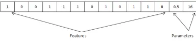
[image:5.612.327.519.283.325.2]If total number of features is N and the number of parameter to be optimized is M, then the length of the chromosome will be N+M. For an exam-ple, we encode a problem in Figure 1. The first 12 bits of the chromosome represent the features and the remaining bits encode the parameters. Each of the first 12 bits represents a feature, and this is randomly initialised to either 0 or 1. If the ith position of a chromosome is 1 then theithfeature participates in constructing the classifier else not. Here out of 12 features, 7 (first, fourth, fifth, sixth, eighth, tenth and eleventh) have been used to con-struct the classifier. If the population size is P then all the P number of chromosomes of this popula-tion are initialized in the same way.
Figure 1: Encoding of the problem
3.4 Fitness Computation
For the fitness computation, the following proce-dure was executed.
(i) Let there are F number of features present in a particular chromosome (i.e. there are total F number of 1’s present in the chromosome).
(ii) Construct a classifier with only these F fea-tures.
(iii). Perform 3-fold cross validation to compute the objective function values.
(iii) The aim is to optimize the values of the objective functions using the search capability of NSGA-II .
3.5 Other Operators
equally important from the algorithmic points of view.
3.6 Selection of Final Solution
MOO provides large number of non-dominated solutions (Deb, 2001) on the final Pareto optimal front. Although each of these solutions are equally important but sometimes the user may require a single solution. Hence, we develop a method for selecting a single solution from the set of solu-tions. For every solution of the final pareto opti-mal front, (i) classifier is trained using the features present in that particular solution (ii) evaluated for 3-fold cross validation on the training set (iii) se-lected the best feature combination that yileds the highest F-measure value and (iv). use this particu-lar feature combination to report the final evalua-tion results.
3.7 Pre-processing and Experimental Setup
The data has to be pre-processed before being used for actual machine learning training. Each tweet is processed to extract only those relevant parts that are useful for sentiment classification. For exam-ple, we removed the tweets that don’t have any la-bel information in the training data; symbols and punctuation markers are filtered out; URLs are re-placed by the word URL; words starting with dig-its are removed etc. Each tweet is then passed through the ARK tagger developed by CMU4for
tokenization and Part-of-Speech (PoS) tagging. From pre-processed tweets we build the final training set. For each tweet in the training set we extract the vectors based on all the features as de-fined above. As the base classifiers we make use of two different learning algorithms, namely Sup-port Vector Machine (SVM) (Vapnik, 1995) and Random Forest (Breiman, 2001). For SVM we use two implementations as available in LibSVM (Chang and Lin, 2011) and LibLINEAR (Rong-En Fan and Hsieh, 2008).
4 Experiments and Result Discussion
In this section we describe the datasets we used for our experiments, report the evaluation results and provide necessary analysis.
4http://www.ark.cs.cmu.edu/TweetNLP/
4.1 Datasets
We use the data sets from SemEval-20145shared
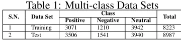
[image:6.612.333.513.198.240.2]task. The data sets contain 8,223 classified tweets in the training data and 8,987 tweets as part of the test data. Details of the data sets are shown in Ta-ble 1. Please note that we make use of our own evaluation script that also considers the accuracies of neutral classes when we perform evaluation. In contrast, the official evaluation of SemEval script simply ignores the neutral classes.
Table 1: Multi-class Data Sets
S.N. Data Set Positive NegativeClass Neutral Total
1 Training 3071 1210 3942 8223 2 Test 3506 1541 3940 8987
4.2 Feature sets
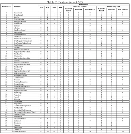
We generate different models using the various feature combinations as shown in Table 2. Brief descriptions of these feature sets are described as below:
S55: is a set of 55 features as listed in Table 2. The intuition behind selection of the features in S55 is described in Section 2.
R20: is a subset of 20 features randomly se-lected from S55.
R30: is a subset of 30 features randomly se-lected from S55.
R40: is a subset of 40 features randomly se-lected from S55.
OS55 with FS & PO: This corresponds to the feature set on which joint feature selection and pa-rameter optimization are performed.
OS55 with default parameters: This corre-sponds to the feature set where feature selection is performed but instead of using parameter op-timization technique we make use of the default parameter settings.
4.3 Parameters for MOO
We use R20, R30 and R40 feature sets to construct the baseline models. Following parameter values are used for the NSGA-II. Population size = 32 ; Number of generations = 20; Number of objective functions = 2; Number of real variables = 2; Prob-ability of crossover of real variable = 0.98; Proba-bility of mutation of real variable = 0.50; Distribu-tion index for crossover = 14; DistribuDistribu-tion index for mutation = 38; Number of binary variables = 55
5http://alt.qcri.org/semeval2014/task9/
Table 2: Feature Sets of S55
Feature No Features R20 R30 R40 S55 OS55 for Exp-PRFeature sets OS55 for Exp-ANF Random
Forest LibSVM LibLINEAR RandomForest LibSVM LibLINEAR
0 HashCount 1 0 1 1 0 0 0 0 0 0
1 TweetLength 1 0 1 1 0 1 0 0 0 0
2 InitCap 0 1 1 1 1 1 1 1 1 1
3 PercentCapital 0 1 0 1 0 1 0 1 1 1
4 AllUpperWword 0 0 1 1 1 0 1 0 0 0
5 NotPresent 0 1 0 1 1 0 0 0 0 0
6 pSmiley 1 0 1 1 0 0 0 1 0 1
7 nSmiley 0 1 1 1 1 1 1 1 1 1
8 LastTokenSmiely 0 1 1 1 1 0 0 1 0 0
9 StopWords 1 0 1 1 0 1 1 0 1 1
10 ElongatedWords 0 1 1 1 1 0 0 0 1 1
11 LastToken 0 0 1 1 1 0 0 0 1 0
12 SwnPositiveTokenCount 1 0 0 1 1 1 0 1 0 0
13 SwnNegativeTokenCount 0 1 1 1 1 1 1 0 1 1
14 SwnNeutralTokenCount 0 0 1 1 1 0 0 1 0 0
15 SwnPolarity 1 1 0 1 1 1 1 1 1 1
16 LexNRC 0 1 1 1 1 1 1 0 1 1
17 PositiveLexNrcToken 1 0 1 1 0 1 0 0 1 0
18 NegativeLexNrcToken 0 1 0 1 0 0 1 1 0 0
19 MaxLexNrc 0 0 1 1 1 1 1 1 1 1
20 MinLexNrc 1 0 1 1 1 1 1 1 1 1
21 LastNonZeroScoreNrc 0 1 1 1 0 0 1 0 0 0
22 Lex140 1 0 1 1 0 0 0 0 0 0
23 PositiveLex140Token 0 1 0 1 1 0 0 0 0 0
24 NegativeLex140Token 0 1 1 1 0 0 0 1 0 1
25 MaxLex140 1 0 1 1 0 0 1 0 0 0
26 MinLex140 0 0 1 1 1 0 0 1 0 0
27 LastNonZeroScore140 0 1 1 1 0 0 0 0 0 0
28 BllPositiveWords 1 0 1 1 1 1 1 1 1 1
29 BllNegativeWords 0 1 0 1 1 1 1 1 1 1
30 CommonNoun 0 1 1 1 1 0 1 1 1 0
31 Pronoun 1 1 0 1 0 1 0 0 1 0
32 NominalPossessive 0 0 1 1 1 0 0 0 1 1
33 ProperNnoun 0 1 1 1 0 0 0 0 0 0
34 ProperNounPossessive 1 1 0 1 1 1 1 1 0 1
35 NominalVerbal 0 0 1 1 1 0 1 1 0 0
36 ProperNounVerbal 0 1 0 1 0 0 1 1 0 1
37 VerbCoupla 1 0 1 1 1 0 0 1 0 0
38 Adjective 0 1 1 1 1 0 1 1 0 1
39 Adverb 0 1 0 1 0 1 0 1 1 0
40 Injection 0 0 1 1 0 1 0 0 1 0
41 Determiner 1 0 1 1 1 0 0 1 0 0
42 Preposition 0 1 1 1 1 0 1 0 0 1
43 ConditionalConjunction 0 0 1 1 0 1 1 0 1 1
44 VerbParticle 1 1 0 1 0 0 0 0 0 0
45 ExistentialPredeterminer 0 1 1 1 0 0 0 0 0 0 46 ExistentialPredeterminerVerbal 0 1 0 1 0 0 0 1 0 0
47 NumberOfHash 1 0 1 1 0 0 0 1 0 1
48 AtMention 1 0 1 1 1 1 1 1 0 1
49 DiscourseMarker 0 1 1 1 1 1 1 1 0 0
50 UrlEmail 1 0 1 1 1 0 0 1 0 0
51 Emoticon 0 1 0 1 1 1 1 1 1 1
52 Numeral 0 1 1 1 1 1 1 1 1 1
53 Punctuaion 0 1 0 1 1 1 0 0 0 1
54 OtherPOS 1 0 1 1 1 1 1 1 1 1
Number of features 20 30 40 55 33 25 26 31 23 26
1 denotes the presence and 0 denotes the absence of a particular feature in the corresponding feature set
4.4 Experimental Results
At first we perform experiments using recall and precision as the two objective functions. Experi-mental results are shown in Table 3. Here we de-fine the three models as follows: Model-1: Ran-dom Forest; Model-2: LibSVM and Model-3: Li-bLinear. The baseline model developed with ran-dom forest classifier shows the highest perfor-mance (i.e. 53.60%) for the system that makes use of 40 features. Random forest based baseline model developed with 20 features (i.e. R20) yields the F-measure values of 50.40% and the model de-veloped with 30 features (i..e R30) shows the F-measure value of 52.30%. With LibLinear
Table 3: Results for Exp-PR
S. N. Feature Sets metersPara- Random Classifiers Forest LibSVM LINEAR
Lib-1 R20 PR 52.1052.70 60.4056.30 49.9053.20 F1 52.30 50.60 50.10 2 R30 PR 50.5050.80 52.3044.60 52.9052.10 F1 50.40 31.00 50.40 3 R40 PR 53.5054.10 58.7053.50 50.5052.20 F1 53.60 46.20 51.00 4 S55 PR 55.1055.60 57.9049.20 53.5055.10 F1 55.10 39.10 53.40 5 with FS & POOS55 PR 62.2061.00 61.0060.60 62.4060.30 F1 59.30 59.10 57.70 6 default paametersOS55 PR 55.5056.10 59.4057.30 62.3060.60 F1 55.50 53.90 58.30 % improvement due to FS 00.40 14.80 04.90
% improvement due to
FS and PO 04.20 20.00 04.30
P=Precision, R=Recall, F1=F-measure (all in %) FS= Feature Selection, PO= Parameter Optimization
Hence it can be concluded that performing fea-ture election and parameter optimisation together is better suited compared to the model that makes use of only the default parameters of the classi-fiers. However, third model achieves higher per-formance with the defaults parameters only. The parameters selected through MOO are shown in Table 5.
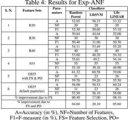
[image:8.612.317.531.48.249.2]Results of the experiments when accuracy and number of features are optimised are shown in Table 4. Results show that both feature selec-tion (FS) and parameter optimizaselec-tion (PO) yield better accuracies with F-measure values of 59.70, 59.20 and 55.50 for the respective models. When the selected feature set is used train the classifiers with default parameters, the models show the F-measure values of 55.50%, 56.10% and 58.00% for the three models, respectively. This again shows quite similar behaviours, i.e. first two classifiers perform superior with the joint model framework. However third model yields higher performance when the classifier is trained with the features selected through MOO based approach, but uses the default parameters.
Here we observe that in both the experiments, LibLinear implementation of SVM provides better result with default parameter configurations com-pared to their respective optimized parameter sets. This may be attributed to the fact that further atten-tion is required to select the parameters of LibLin-ear model. Our approach is evolutionary in nature, and therefore, better accuracies can be achieved by either increasing the number of generations or size of the population or both.
Table 4: Results for Exp-ANF
S. N. Feature Sets metersPara- Random Classifiers Forest LibSVM LINEAR
Lib-1 R20 NFA 52.6520 56.3320 53.3220 F1 52.30 50.60 53.10 2 R30 NFA 50.8430 44.6430 52.0030 F1 50.40 31.00 50.30 3 R40 NFA 54.1140 53.4940 55.2040 F1 53.60 46.20 54.10 4 S55 NFA 55.6155 49.255 54.1655 F1 55.10 39.10 49.90 5 with FS & POOS55 NFA 61.3231 60.5823 59.0626 F1 59.70 59.20 55.50 6 default paametersOS55 NFA 56.0831 58.5323 60.2426 F1 55.50 56.10 58.00 % improvement due to FS 00.40 17.00 08.10
% improvement due to
FS and PO 04.60 20.10 05.60
A=Accuracy (in %), NF=Number of Features, F1=F-measure (in %), FS= Feature Selection, PO=
Parameter Optimization
Table 5: Optimized Parameters
S.N. Classifier Parameters Exp-PR ExperimentExp-ANF
1. Random Forest Trees 862, 853 1990 2. LibSVM GammaCost 2ˆ(-10)2ˆ14 2ˆ(-9)2ˆ14 3. LibLINEAR Cost 4 2ˆ(-2), 2ˆ(-7), 2ˆ(-8)
4.5 Comparisons
tem II’. Here ’Our System I’ has much better F-measure than the average F-F-measure of our system which ignores the neutral class. This shows that our system provides better F-measure for neutral class.
Table 6: Comparisons with some existing systems
S.
N. System Live F-measure
Jou-rnal 2014
SMS 2013
Twi-tter 2013
Twi-tter 2014
Twitter 2014 Sar-casm
Ave-rage
1. NRC Canada-B 74.84 70.28 70.75 69.85 58.16 68.78 2. Coooolll-B 72.90 67.68 70.40 70.14 46.66 65.55 3. TeamX-B 69.44 57.36 72.12 70.96 56.50 65.27 4. SAIL-B 69.34 56.98 66.80 67.77 57.26 63.63 5. Our System I 64.16 74.75 68.39 60.62 35.48 60.68 6. SU-sentilab-B 55.11 49.60 50.17 49.52 31.49 47.18 7. Our System II 57.77 45.00 49.40 47.84 25.76 45.15 8. DAEDALUS-B 40.83 40.86 36.57 33.03 28.96 36.05
5 Conclusion and Future Work
In this work, we have posed the problem of si-multaneous feature selection and parameter opti-mization as a MOO problem, and evaluate this for sentiment analysis. We have implemented signif-icantly diverse set of features for the task. Ex-periments show the effectiveness of the proposed approach with significant performance improve-ments over the various baselines developed with random feature subsets. It is also evident from the evaluation results that simultaneous feature se-lection and parameter optimization is better com-pared to the only feature selection.
In future, we would like to add more features to increase the baseline performance. More detailed parameter selection, for example, the kernel func-tion of SVM need to be optimised to realise the ef-fects of more systematic parameter optimization.
Acknowledgments
We thank the anonymous reviewers for their com-ments. This work is, in part, supported by German Academic Exchange Service (DAAD) through DAAD-IIT Master Sandwich Program.
References
[Alec Go and Huang2009] Richa Bhayani Alec Go and Lei Huang. 2009. Twitter sentiment classification using distant supervision. Technical report, Univ. stanford.
[Andrea Esuli and Sebastiani2010] Stefano Baccianella Andrea Esuli and Fabrizio Sebastiani. 2010. Senti-wordnet 3.0: An enhanced lexical resource for sen-timent analysis and opinion mining. InSeventh
con-ference on International Language Resources and Evaluation LREC’10, Valletta, Malta, May.
[Apoorv Agarwal and Passonneau2011] Ilia Vovsha Owen Rambow Apoorv Agarwal, Boyi Xie and Rebecca Passonneau. 2011. Sentiment analysis of twitter data. In Proceedings of the Workshop on Languages in Social Media, pages 30–38. Association for Computational Linguistics.
[Bo Pang and Vaithyanathan2002] Lillian Lee Bo Pang and Shivakumar Vaithyanathan. 2002. Thumbs up?: sentiment classification using machine learn-ing techniques. InProceedings of the ACL-02 con-ference on Empirical methods in natural language processing-Volume 10, pages 79–86. Association for Computational Linguistics.
[Boiy and Moens2009] Erik Boiy and Marie-Francine Moens. 2009. A machine learning approach to sen-timent analysis in multilingual web texts. Informa-tion retrieval, 12(5):526–558.
[Breiman2001] Leo Breiman. 2001. Random forests. Mach. Learn., 45(1):5–32, October.
[Buckland and Gey1994] Michael K. Buckland and Fredric C. Gey. 1994. The relationship between re-call and precision.JASIS, 45(1):12–19.
[Cataldo Musto and Polignano2014] Giovanni Semer-aro Cataldo Musto and Marco Polignano. 2014. A comparison of lexicon-based approaches for senti-ment analysis of microblog posts. Information Fil-tering and Retrieval, page 59.
[Chang and Lin2011] Chih-Chung Chang and Chih-Jen Lin. 2011. Libsvm: A library for support vector ma-chines. InACM Transactions on Intelligent Systems and Technology.
[CHRIS NICHOLLS2009] FEI SONG CHRIS NICHOLLS. 2009. Improving senti-ment analysis with part-of-speech weighting. In Eighth International Conference on Machine Learning and Cybernetics, Baoding, July.
[Deb2001] Kalyanmoy Deb. 2001. Multi-objective Optimization Using Evolutionary Algorithms. John Wiley and Sons, Ltd, England.
[Dmitry Davidov and Rappoport2010] Oren Tsur Dmitry Davidov and Ari Rappoport. 2010. En-hanced sentiment learning using twitter hashtags and smileys. InColing 2010: Poster Volume, pages 241–249, Beijing, August.
[Ekbal and Saha2012] Asif Ekbal and Sriparna Saha. 2012. Multiobjective optimization for classifier ensemble and feature selection: an application to named entity recognition.IJDAR, 15(2):143–166.
[Ekbal and Saha2013] Asif Ekbal and Sriparna Saha. 2013. Full length article: Simulated annealing based classifier ensemble techniques: Application to part of speech tagging.Inf. Fusion, 14(3):288–300, July.
[Gizem Gezici and Saygin2013] Berrin Yanikoglu Dilek Tapucu Gizem Gezici, Rahim Dehkharghani and Yucel Saygin. 2013. Su-sentilab: A classi-fication system for sentiment analysis in twitter. In Proceedings of the International Workshop on Semantic Evaluation, pages 471–477.
[Hassan Saif and Alani2012] Yulan He Hassan Saif and Harith Alani. 2012. Semantic sentiment analysis of twitter. In11th international conference on The Semantic Web ISWC’12, Volume I, Heidelberg.
[JulioVillena Roman2014] Gonzalez Cristobal Jose Carlos JulioVillena Roman, Janine Gar-cia Morera. 2014. Daedalus at semeval-2014 task 9: Comparing approaches for sentiment analysis in twitter.
[Kevin Gimpel2011] Nathan Schneider Kevin Gimpel. 2011. Part-of-speech tagging for twitter: Annota-tion, features, and experiments. InProceeding HLT ’11 Proceedings of the 49th Annual Meeting of the Association for Computational Linguistics: Human Language Technologies: short papers - Volume 2 Pages 42-47.
[Liu and Motoda1998] Huan Liu and Hiroshi Motoda. 1998. Feature Selection for Knowledge Discovery and Data Mining. Kluwer Academic Publishers, Norwell, MA, USA.
[Liu and Yu2005] Huan Liu and Lei Yu. 2005. Toward integrating feature selection algorithms for classifi-cation and clustering. IEEE Trans. on Knowl. and Data Eng., 17(4):491–502.
[Maite Taboada and Stede2011] Milan Tofiloski Kim-berly Voll Maite Taboada, Julian Brooke and Man-fred Stede. 2011. Lexicon-based methods for sentiment analysis. Computational linguistics, 37(2):267–307.
[Maks and Vossen2013] Isa Maks and Piek Vossen. 2013. Sentiment analysis of reviews: Should we an-alyze writer intentions or reader perceptions? In RANLP, pages 415–419.
[Mitchell1997] Thomas M. Mitchell. 1997. Machine Learning. McGraw-Hill, Inc., New York, NY, USA, 1 edition.
[Mittal and Goel2012] Anshul Mittal and Arpit Goel. 2012. Stock prediction using twitter sentiment anal-ysis.Standford University.
[Miura et al.2014] Yasuhide Miura, Shigeyuki Sakaki, Keigo Hattori, and Tomoko Ohkuma. 2014. Teamx: A sentiment analyzer with enhanced lexicon map-ping and weighting scheme for unbalanced data. In Proceedings of the 8th International Workshop on Semantic Evaluation (SemEval 2014), pages 628– 632, Dublin, Ireland, August. Association for Com-putational Linguistics and Dublin City University.
[Mukherjee and Bhattacharyya2012] Subhabrata Mukherjee and Pushpak Bhattacharyya. 2012. Fea-ture specific sentiment analysis for product reviews. In Computational Linguistics and Intelligent Text Processing, pages 475–487. Springer.
[Nielsen2011] F. ˚A. Nielsen. 2011. Afinn. Technical report, Richard Petersens Plads, Building 321, DK-2800 Kgs. Lyngby, March.
[Nikolaos Malandrakis and Narayanan2014] Colin Vaz Jesse Bisogni Alexandros Potamianos Niko-laos Malandrakis, Michael Falcone and Shrikanth Narayanan. 2014. Sail: Sentiment analysis using semantic similarity and contrast. SemEval 2014, page 512.
[Pak and Paroubek2010] Alexander Pak and Patrick Paroubek. 2010. Part-of-speech tagging for twitter: Annotation, features, and experiments. InSeventh International Conference on Language Resources and Evaluation, LREC 2010.
[En Fan and Hsieh2008] Kai-Wei Chang Rong-En Fan and Cho-Jui Hsieh. 2008. Liblinear: A library for large linear classification. InJournal of Machine Learning Research.
[Saif Mohammad and Zhu2013] Svetlana Kiritchenko Saif Mohammad and Xiaodan Zhu. 2013. Nrc-canada: Building the state-of-the-art in sentiment analysis of tweets. InProceedings of the seventh in-ternational workshop on Semantic Evaluation Exer-cises (SemEval-2013), Atlanta, Georgia, USA, June.
[Tang et al.2014] Duyu Tang, Furu Wei, Bing Qin, Ting Liu, and Ming Zhou. 2014. Coooolll: A deep learn-ing system for twitter sentiment classification. In Proceedings of the 8th International Workshop on Semantic Evaluation (SemEval 2014), pages 208– 212, Dublin, Ireland, August. Association for Com-putational Linguistics and Dublin City University.
[Vapnik1995] Vladimir N. Vapnik. 1995. The nature of statistical learning theory. Springer-Verlag New York, Inc., New York, NY, USA.
[Xiaodan Zhu and Mohammad2014] Svetlana Kir-itchenko Xiaodan Zhu and Saif M Mohammad. 2014. Nrc-canada-2014: Recent improvements in the sentiment analysis of tweets. SemEval 2014, 443.
[Xiaowen Ding and Yu2008] Bing Liu Xiaowen Ding and Philip S Yu. 2008. A holistic lexicon-based approach to opinion mining. InProceedings of the 2008 International Conference on Web Search and Data Mining, pages 231–240. ACM.