Three Equivalent Codes for Autosegmental Representations
Anssi Yli-Jyr¨
a
Department of Modern Languages, University of Helsinki, Finland
[email protected]Abstract
A string encoding for a subclass of bi-partite graphs enables graph rewriting used in autosegmental descriptions of tone phonology via existing and highly opti-mized finite-state transducer toolkits (Yli-Jyr 2013). The current work offers a rig-orous treatment of this code-theoretic ap-proach, generalizing the methodology to all bipartite graphs having no crossing edges and unordered nodes. We present three bijectively related codes each of which exhibit unique characteristics while pre-serving the freedom to violate or express the OCP constraint. The codes are in-finite, finite-state representable and opti-mal (efficiently computable, invertible, lo-cally iconic, compositional) in the sense of Kornai (1995). They extend the encod-ing approach with visualization, general-ity and flexibilgeneral-ity and they make encoded graphs a strong candidate when the for-mal semantics of autosegmental phonology or non-crossing alignment relations are im-plemented within the confines of regular grammar.
1
Introduction
1.1 Autosegmental Phonology
Historically, Autosegmental Phonology (Gold-smith, 1976) helped to articulate theindependence of the melody, thedecomposition of contour tones as level tones and theObligatory Contour Princi-ple (OCP) that bans adjacent copies of phonolog-ical units. Its multi-tiered design was also a cru-cial step towards more complex phonological the-ories such as Feature Geometry (Clements, 1985), Optimal Domains Theory (Cassimjee and Kisse-berth, 1998) and Autosegmental-Metrical Theory (Ladd, 2008). Moreover, autosegmental represen-tations are timelessly interesting formal objects as they are similar to certain alignment relations aris-ing in statistical machine translation.
Autosegmental Phonology continues to play an appreciated role in language documentation efforts
for under-resourced languages. In particular, de-scribing Bantu tone is extremely complex (Nurse and Philippson, 2003) as the lexical, morphologi-cal, phonological and syntactic dimensions of each language are intertwined in unique ways although there are tonological characteristics shared across the Bantu family. Many prior accounts have re-lied on autosegmental rules while constraint-based approaches sometimes offer an equivalent solution only too painfully via varying constraint rank-ings. After all, languages with a young or de-veloping orthography urgently need lexical trans-ducers (Beesley and Karttunen, 2003) and, es-pecially, tonologically enriched lexical transducers (Hurskainen, 2009; Muhirwe, 2010) that can be used to improve speech applications and various text normalization tools. It is, therefore, desirable that tone processing is incorporated into existing and highly optimized finite-state toolkits and lex-ical databases that have been primarily designed for segmental phonology and morphology.
According to Autosegmental Phonology, phono-logical tone is not a feature inside a phonemic seg-ment, but rather a segment in its own right – thus anautosegment. The phonological representation consists of aligned tiers of strings: the autosegmen-tal tonemes lying in one tier are associated with segmental phonemes in the other tier. For clar-ity, we naively discard the actual phonological and metrical values of tone bearing units (TBUs) in the segmental tier. A possible way to associate the tone stringHLHLHwith the segmental stringVVVVVV is given by the autosegmental representation
H
V L
∅ ∅
V V
H L
V V H
V
. (1)
The notion of autosegments formalizes five im-portant characteristics (Yip, 2002) of the tone-segment relationship:
1. “mobility”: The alignment between tones and segments is mutable.
3. “toneless segments”: A segment can be temporarily unattached to a tone.
4. “one-to-many”: A tone can be associated with multiple segments.
5. “many-to-one”: Many tones can be associ-ated with a single segment.
Until recently, autosegmental processing ap-peared to require advanced computational repre-sentations and a graph rewriting system. Conse-quently, the lack of a usable finite-state implemen-tations has remained as a bottleneck.
1.2 Prior Computational Approaches
A few computational implementation approaches for autosegmental representation have been pro-posed. For example, there are software systems such as the Delta programming language (Hertz, 1990), AMAR (Albro, 1994) and Tone Pars (Black, 1997). These systems do not explicitly rely on automata, but there are other computational ap-proaches that are clearly related to finite automata and transducers:
1. OCP-bound finite-state approaches (Bird and Klein, 1990; Bird and Ellison, 1994; Bird, 1995; Carson-Berndsen, 1998; Jardine, 2013) hardwire the Obligatory Contour Principle into their mathematical formalization of au-tosegments. The principle was originally mo-tivated by Leben (1973), but its status as a universal constraint has been under scrutiny ever since (see McCarthy 1986).
2. OCP-neutral finite-state approaches (Kor-nai, 1995; Wiebe, 1992; Yli-Jyr¨a, 2013) see that the OCP is sometimes violated unless not maintained by the rules (Odden, 1986). OCP-neutral approaches have been advocated (Goldsmith, 1976; Odden, 1986; Prince and Smolensky, 2004) and it is sometimes assumed by field linguistic descriptions (Halme, 2004).
Both approaches have their merits. Since our in-terest is in extending the capacity of generic finite-state toolkits towards tonology rather than to de-velop a principled phonological theory, the OCP-neutral approach is now preferred.
The main prior contributions towards the im-plementation of the OCP-neutral approach can be summarized as follows:
• Wiebe (1992) and Kornai (1995) model au-tosegmental representations via multi-tape automata and the corresponding codes.
• Yli-Jyr¨a (2013) adopts some simplifying as-sumptions and then models the representa-tions as bracketed strings.
The bracket encoding of Yli-Jyr¨a (2013) is practi-cally implemented and compatible with the stan-dard technology for building lexical transducers. Unfortunately, it supports only a particular subset of all two-tiered autosegmental representations.
1.3 The Limits of the Prior Work
In the bracket-based encoding of Yli-Jyr (2013), the edge of each tone is indicated with a corre-sponding bracket. For example, the representation (1) reduces to string [V]()V[V)[VVV]. When we replace symbols()[]withHH LL, respectively, this string reduces toHVH LLVHVL HVVVH.
It is not difficult to see that the encoding scheme has some limitations that prompt further research:
• The approach is not expressed and analyzed in terms of coding theory. Therefore, the issue of existence of acompositional coding function (Kornai, 1995) was not properly addressed.
• The encoding does not capture some tone configurations of autosegmental bipartite graphs: complex contour tones, skipping of unlinked vertices and zigzag chaining:
V H L H
V V H
V H
V L
V.
• Associations and respective changes must be hand-encoded, while the original formalism (Goldsmith, 1976) is graphical and it indicates insertions (...) and removals () intuitively by
graphical signs such as:
V V
H
H L
.
In the encoding, there is also a limitation that is mainly useful. Namely, the encoding does not equate the autosegmental representations
H
∅ ∅
V
and
∅
V H
∅.
Instead, the order of unlinked elements is mean-ingful: HHV6=VHH. This property that we now call
Inertia means that the order of isolated vertices
is fixed by the way in which they are concatenated and changed only by force: via rewriting. As the shuffling of floating tones and toneless segments is now delegated to the rules, the OCP-neutral sentations are fully linearizable although the repre-sentations discussed by Wiebe (1992) and Kornai (1995) are not.
1.4 The Results of This Paper
(Berstel et al., 2010) in order to get formal results that are fundamental to a practical finite-state im-plementation such as Yli-Jyr (2013).
The first consequence (Section 3) of this ap-proach is that there is anoptimal coding func-tion (Kornai, 1995) for inertial autosegmental graphs that are generated by an appropriately de-finedinfinite source “alphabet”.
The second major result is that aserial code with an optimal coding function can also be visually at-tractive (Section 4). Our visual code is easy to read and write. This is handy as no separate visu-alization step is required to make the code human readable.
The third major result is that the previously pre-sented bracket encoding extends to all non-crossing link configurations via the symmetric bracket code that supports complex contours, skipping and chaining (Section 5).
We will also see that the visual code and the symmetric bracket code are bijectively related via a Polish codethat is a simple, computationally motivated code (Section 6).
2
Definitions
2.1 Autosegmental Graphs
Different axiomatizations for autosegmental graphs have been proposed since Goldsmith (1976). In particular, the Non-Crossing
Con-straint (NCC) is a common assumption in
autosegmental theory, although it has been con-tested in prosodic morphology (Bagemihl, 1989; McCarthy and Prince, 1996).
For us, the tone-segment associations are for-malized as bipartite graphs whose vertices are (auto)segments. The sets of vertices are ordered in each graph since they correspond to tonal and seg-mental strings. In addition, the associating edges between them are ordered due to the NCC. The vertices without incident edges are called isolates and they are ordered due to theInertiaproperty that was implicit already in Yli-Jyr (2013) but is now formalized for the first time.
Definition 1. An autosegmental graphis
• a bipartite graphG= (T∪V, E,≤T,≤V,≤E) with verticesT∪V and undirected edgesE⊆ T×V,
• with total order≤T forT and≤V forV,
• with total order ≤E of edges E satisfying (v, v0) ≤ (u, u0) ↔ v ≤ u∧v0 ≤ u0 for all
(v, v0),(u, u0)∈E.
If there is a total order ≤I over (T ∪V)− {e | (e, f)∈ E}, G= (T ∪V, E,≤T,≤V,≤E,≤I) is an autosegmental graph withInertia.
Concatenation of disjoint a.s. graphs is defined by extending the ≤-relations in a natural way, by concatenating the ordered sets of tones, vowels, edges and isolates.
2.2 Coding Functions
Kornai (1995) has formalized computational imple-mentation of autosegmental graphs as a problem of finding a coding function β such that for any au-tosegmental graphG(called abistring by Kornai), its imageβ(G) is a string over a finite alphabetA. There are infinitely many possible coding func-tions, but Kornai narrows the task with four prop-erties characterizingan optimal coding function βˆ:
1. ˆβ is computablee.g. by a Turing Machine; ideally, the computation is carried out in real time, e.g. with a finite state transducer.
2. ˆβ is invertiblei.e. at least injective; ideally, this means that function ˆβ is even bijective.
3. ˆβisiconici.e. analogical rather than cryptic; ideally, a local change in G corresponds to a local change in ˆβ(G).
4. ˆβ is compositional i.e. it is a mor-phism that respects concatenation: ˆβ(GG0) =
ˆ
β(G) ˆβ(G0).1
It is impossible to construct an ideal coding func-tion for autosegmental graphs in general (Kornai, 1995). The lack of compositionality holds even when these graphs are edgeless (Wiebe, 1992). This relates to the fact that the Cartesian prod-uctA∗×B∗is not equidivisible and thus not a free monoid (Sakarovitch, 2009).
2.3 Towards a Monoid Morphism
Although there is no compositional coding function for all autosegmental graphs (Wiebe, 1992), we will now exploit coding theory (Berstel et al., 2010) to find a class of autosegmental graphs for which a compositional coding function exists.
Let A be an alphabet. A subset X ⊆ A∗ is a code over A if every word w ∈ X∗ is written uniquely as a product of words in X. In other words, for x1, . . . , xn, y1. . . ym ∈X, the condition
x1. . . xn=y1. . . ymimpliesn=mandxi=yifor all li∈ {1, .., n}.
Observe that if the concatenation does not add any new edges to disjoint graphs under the oper-ation, there must be a separate code element for every connected graph. Since the set of connected graphs is infinite, a block code is not possible, but the code must beinfinite. In addition, possible iso-lates intervening any pair of nodes of a connected
1Beware the terminology: a coding functionβ can
component must be coded along with the compo-nent.
An infinite code is perfectly normal notion (Bers-tel et al., 2010) although it requires more than a finite table (for example, a graph serialization algo-rithm). For example, themaximal semaphore code
X =A∗S−A∗SA+ for a semaphore set S ⊆A+
is infinite at least whenS ⊂A. Furthermore, any infinite or finite subset of some infinite code is also a code and can be sufficient when the source text is limited — e.g., a finite data set or a specific natural language.
A morphism β : H∗ → A∗ from a monoid (H∗,·, ) into a monoid (A∗,·, ) is a coding mor-phism for a codeX ⊆A∗ if
1. β is injective and, thus, preserves the distinc-tiveness of the elements ofH, and
2. X =β(H), i.e., every code word corresponds to a letter inH (Berstel et al., 2010).
Theorem 1. Let β : H∗ →A∗ be a coding
mor-phism for a codeX ⊆A∗. Thenβ is an invertible and compositional coding function (Kornai, 1995).
Proof. Every morphism is compositional since the conditionβ(hh0) =β(h)β(h0) for all h, h0 ∈H∗ is a part of the definition of morphisms. Moreover, invertibility follows from the definition of a coding morphism.
2.4 The Approach
Our current code theoretic approach can be sum-marized as follows:
1. No free floating. Since the graphs must cor-respond to uniquely tokenizable code words, we will restrict ourselves to the autosegmen-tal graphs withInertia.
2. Infinite source alphabet and code. Theo-rem 1 and the previous negative results guide us to reject the prior assumption about a fi-nite code (Kornai, 1995) and look for an in-finite code X and an infinite source alpha-bet H consisting of certain kinds of graphs. The resulting approach differs vastly from ap-proaches that enforce a finite source alphabet and the OCP (e.g. Bird and Ellison 1994).
3. Finite channel alphabet. Defining mor-phisms from an infinitely generated monoid may seem scary, as formal languages are usu-ally subsets of finitely generated free monoids. However, after the graphs are encoded by a code X∗ that is subset of a finitely generated monoidA∗, they can be manipulated via finite state relations over subsets ofA∗.
3
Codability of Graphs
We will now choose a source alphabetH in such a way that it generates a free monoid (H∗,·, ) and
coincides with our autosegmental graphs.
3.1 Non-trivial Connected Components
Theorem 2. All connected components of autoseg-mental graphs are trees.
Proof. Assume that there is a connected autoseg-mental graph that is not a tree. Such a bipartite graph must contain a cycle that involves at least four vertices and there is a crossing edge; contra-diction.
Define the relation ≤S over connected compo-nentsC and C0 of a graph Gin such a way that C ≤S C0 if C = C0 or every edge in C is before every edge inC0. The relation≤S is reflexive, tran-sitive and antisymmetric, thus a partial order.
Theorem 3. The≤S-order of nontrivial (contain-ing at least two vertices) connected components of an autosegmental graph is a total order.
Proof. LetCandC0 be nontrivial connected com-ponents for which C 6≤S C0 and C0 6≤S C. Then there are distinct edges (s, s0),(t, t0)∈C, (u, u0)∈ C0or edges (s, s0),(t, t0)∈C0, (u, u0)∈Csuch that (s, s0)<E (u, u0)<E (t, t0). Since vertices sand t are connected and there are no crossing edges, they are connected to vertices u and u0. This means, however, that C = C0; contradiction. Thus, the
order≤S is total.
3.2 Embracements
An isolate vertex y is embraced by a connected component C ifC contains verticesxand z such that x ≤T y ≤T z or x ≤V y ≤V z. We extend every connected componentCof an autosegmental graph into a subgraph C0 called an embracement by adding toC0 all isolates embraced byC.
Corollary 1. Every autosegmental graph consists of a totally ordered set of embracements.
Thus, we obtain acomplete set of generatorsfor all autosegmental graphs by expanding the con-nected components with embraced isolates. This infinite set of generatorsHis such that an optimal coding function ˆβ :H∗→A∗ is possible.
4
New Codes for the Graphs
4.1 The Visual CodeThe visual code is defined over the alphabet
A={(/V),(\ T),(|VT),(-V),(.V),
(- T),(T)}
=
/ V,
T
\,T| V,
-V,
. V,
T -, T
The idea is that autosegmental graphs such as
V T T T
V V T V ∅ V T V T V T ∅ (2)
are encoded as visually similar strings:
T
\ T\ T| V / V -V T | V . V T \ / V T | V T .
The code is infinite and has a value for every possible embracement. The code word for each embracement ends with one of the semaphores
S = {(.V),(T),(|VT)}. Corresponding to this, we designate one of the rightmost vertices as the root for any non-trivial tree in the embracement. The code word for an embracement is constructed leftwards from this vertex as explained in Table 1. The resulting set of code words is given by regular expression2
X =
. V
[T [
/ V -V ∗ [T
\ T -∗∗
T | V.
This set is recognized by the automaton in Fig. 1.
0
1 (°T) (∅V)
2 ε (|VT) 3 (/ V) 4 (\ T) ε (-V ) ε (- T)
Figure 1: Recognizer for the visual code
Theorem 4. The languageX is a code.
Proof. The set X is a subset of the maximal semaphore code A∗S −A∗SA+ with semaphores
S. Thus,X is a code.
4.2 The Symmetric Bracket Code
The alphabet of the symmetric bracket code is
B ={[,],V,V,}. As the vowels and tones reduce to paired symbols i.e. brackets, both vertex types are treated symmetrically as autosegments. For ex-ample, (2) is encoded with the symmetric bracket code as
V[][][V] V[VVVVV] VV V[][VVV] [].
The code word for each embracement ends with a closing tone bracket (]) or a closing vowel bracket
2Here the regular expression operators are:
[image:5.595.306.529.80.334.2]concate-nation, union (∪), star (∗), kleene plus (”+”), differ-ence (−), and grouping ({}).
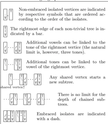
Table 1: Encoding a graph with the visual code
. V,
T Non-embraced isolated vertices are indicated
by respective symbols that are ordered ac-cording to the order of the isolates.
T | V
The rightmost edge of each non-trivial tree is in-dicated by a bar.
/ V· · ·
/ V T | V
Additional vowels can be linked to the tone of the rightmost vertice (the natural limit is, however, three tones).
T
\· · · T\ T| V
Additional tones can be linked to the vowel of the rightmost vertice.
T
\ · · · T\ / V
shared vertex↑
· · ·/ V T | V
Any shared vertex starts a new subtree.
· · · / V T
\· · · T\ / V· · ·
/ V T
\· · · There is no limit for thedepth of chained sub-trees. / V -V T | V T
\ T- T| V
Embraced isolates are indicated with a dash.
(V). The code word for an embracement is con-structed as explained in Table 2. The resulting set of code words is
Z =
VV [ []
[ V[ ] [] ∗
[ [ V
VV ∗ V ∗ V].
Theorem 5. The languageZ is a code.
Proof. The finite automaton in Figure 2 recognizes the languageZ. Although the drawn automaton is not deterministic, it is easy to verify that it recog-nizes a prefix-free stringset — thus a code (Berstel et al., 2010).
0 1
V̅
2 V̅V, [ ]
3 [ 4 ] 5 V [ [°] ] V̅ 6
V̅°V
V̅
V̅°V
Figure 2: Recognizer for the bracket code
4.3 The Polish Code
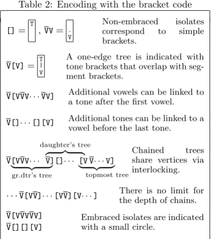
Table 2: Encoding with the bracket code
[]= T , VV= . V
Non-embraced isolates
correspond to simple
brackets.
V[V]=
T | V
A one-edge tree is indicated with tone brackets that overlap with seg-ment brackets.
V[VVV· · ·VV] Additional vowels can be linked to a tone after the first vowel.
V[]· · ·[][V] Additional tones can be linked to a vowel before the last tone.
V[VVV· · ·
| {z }
gr.dtr’s tree
daughter’s tree
z }| {
V][]· · · [V V· · ·V]
| {z }
topmost tree
Chained trees
share vertices via interlocking.
· · ·V[VV]· · ·[VV][V· · ·] There is no limit for
the depth of chains.
V[VVVVV] V[][][V]
Embraced isolates are indicated with a small circle.
Our Polish code is defined over the alphabetD=
[image:6.595.305.521.86.213.2] [image:6.595.316.518.327.395.2] [image:6.595.335.495.698.734.2]{|, ,V,T}. For example, (2) is encoded as
|T|T|VT |VV|VT V |T|V|VT T. (3)
Every edge (|) acts twice as an operand: for two kinds of variadic operators, a tone (T) and a vowel (V). One of these operators must be applied imme-diately to each edge, but the other operator is later applied to all edges that have not been operated on. If an operator would otherwise have some operands available, it can be forced to apply tono operands (edges) through a -prefix. In order to avoid spu-rious ambiguity, sequences|VT,|VT· · ·T,|VTV· · ·V are equated with their non-normalized equivalents
|TV,|T· · ·TV,|VV· · ·VTthat will be excluded from
the code. The code word for an embracement is constructed as explained in Table 3. The resulting set of code words is
Y =|
V
V
∗
| [ T
T
∗
|
∗
VT [
V,T
.
These code words are recognized by the finite au-tomaton in Figure 3.
0 1 |
2 T V
3 T
4 V |
°T
|
T 5 °V |
°V
Figure 3: Recognizer for the Polish code
Theorem 6. The languageY is a code.
Proof. The language Y is a prefix code, thus, a code: Y ∩Y D+=∅ (Berstel et al., 2010).
Table 3: Encoding a graph with the Polish code
T,V Non-embraced isolates are nullary operators.
|VT A one-edge tree consists of an edge and two
vertices.
|V· · ·|V|VT Additional vowels can be linked.
|T· · ·|T|VT Additional tones can be linked.
|T|V|V|T|T|V|VT Trees can be chained.
|VV|VT |TT|VT
Embraced isolates are nullary opera-tors.
5
Equivalences
In this section, we show that the autosegmental graphs withInertiahave linear time coding func-tions to the three codes presented above. In ad-dition, we show that the bijections between the codes are finite-state computable. This results into equivalences in Figure 4.
A.s. graphs
Thm. 10 ↔ l Thm. 7
↔
Thm. 10
Visual code
Cor. 2 ↔ Thm. 9
↔
Thm. 8
Polish code ←→ Bracket code
Figure 4: The equivalence results
Theorem 7. There is a linear time bijection be-tween the visual code and the set of possible em-bracements in autosegmental graphs.
Proof. LetG= (T ∪V, E,≤T,≤V,≤E,≤I) be an autosegmental graph with Inertia. Compute a partial order≤F overT∪V in such a way that
y <F z if and only if∃(y, z),(x, z)∈E s.t.
y <T xor y <V x
y=F z if and only if∃(y, z)∈E s.t
∀(x, z),(y, v)∈E we have
(x, z)≤E(y, z) and (y, z)≤E (y, z).
Let G0 = (T ∪V,≤T ∪ ≤V ∪ ≤I ∪ ≤F) be a di-rected graph. If this didi-rected graph contains cycles they are between =F -equivalent vertices. In order to be able to view the graph as an acyclic graph and sort it topologically, we temporarily eliminate each cycle by unifying the vertices in it. This re-sults into a graph with position indexes:
V3
T1 T2 T3
V4V5V6
T6 ∅
V7 V9V10
T8 T10
∅
T11
For example,T3andV3in this graph are are viewed
during the sorting procedure. Using the position indexes of the vertices, we encode each position with an element of the alphabet A of the visual code. In total, the encoding is computed in deter-ministic linear time.
Conversely, letw ∈X∗ be a visual code string.
We construct an autosegmental graph G = (T ∪ V, E,≤T,≤V,≤E,≤I) from it: The boxes are bered rightward by positive integers. These num-bers give indices to the vertices. Then we ex-tract, from w, the edges by complementing each partial edge with the closes missing vertex to the right. Then the total orders ≤T,≤V,≤E,≤I are extracted in the obvious way by a finite number of scans through the string.
For example, the visual code string
T1
\ T\2 T|3 V3 / V4 . V5 T6 | V6 . V7 T8 \ / V9 T10 | V10 T11
gives rise to the autosegmental graph G = (T ∪ V, E,≤T,≤V,≤E,≤I) with
• the ≤T-ordered set of tone vertices T =
hT1,T2,T3,T6,T8,T10,T11i
• the ≤V-ordered set of vowel vertices V =
hV3,V4,V5,V6,V7,V9,V10i,
• the ≤E-ordered set of edges E = h(T1,V3),
(T2,V3), (T3,V3), (T6,V4), (T6,V6), (T8,V9),
(T10,V9), (T10,V10)i,
• the≤I-order over isolates: V5<V7<T11.
Theorem 8. There is a finite state bijection be-tween the Polish code and the visual code.
Proof. Figure 5 shows a finite state transducer mapping the language Y∗
[image:7.595.304.526.113.237.2]0 T:(° T) V:(.V ) 1 |:ε 2 V:(/ V) 3 V:(|VT) 4 T:(\ T) |:ε °V:(-V ) T:ε |:ε °T:(- T)
Figure 5: Y∗↔X∗
to language X∗. It is easy to verify that both the transducer and its inverse are functions. In addition, it is possible to verify mechanically that the preimage and the image of this func-tion are exactlyY∗and
X∗, respectively. Thus, it defines a bijection.
The transducer in Figure 5 is constructed with the 2-tape regular expression3:
|:
T:(\ T) T:(- T)∗|: ∪
V:(/ V) V:(-V )∗ |:
∗
V:(|VT) T:
∪
T:( T)∪V:(. V)
∗
3The additional operators are: cross product (:),
and composition (◦)
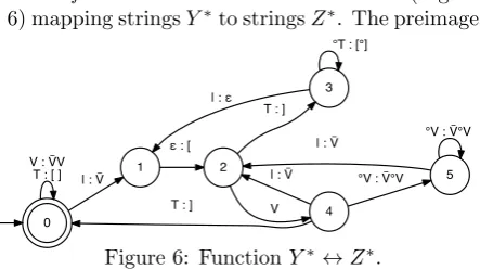
Theorem 9. There is a finite state bijection be-tween the Polish code and the symmetric bracket code.
Proof. There is a finite state transducer (Figure 6) mapping stringsY∗to stringsZ∗. The preimage
0 V : V̅V
T : [ ] | : V̅ 1 2 ε : [
3 T : ]
4 V | : ε
°T : [°]
T : ]
| : V̅ °V : V̅°V 5 | : V̅ °V : V̅°V
Figure 6: FunctionY∗↔Z∗.
and the image of this function areY∗ andZ∗, re-spectively. It is easy to verify that both the trans-ducer and its inverse are total functions. Thus, it defines a bijection.
The transducer in Figure 6 is constructed by the 2-tape regular expression
Y∗◦
(B\{|∪T∪ }) ∪ T:[] ∪T:[]∪V
∪
| {:[} {B\T}∗ {T:]}
∗ ◦
(B\{|∪V}) ∪ V:VV ∪ V:VV
∪
|:V {B\V}∗ {V:V} ∗ ◦
(B\|) ∪ |:
∗
.
[image:7.595.74.288.656.742.2]that implements the following intuition: (1) start with Y∗; (2) add tone brackets; (3) add vowel brackets; (4) remove the remaining |-symbols. When these steps are applied to input string (3), we obtain the following derivation:
|TT|VT |VV|VT V |T|V|VT T⇒ |[][]|[V] |[VV|V] V |[]|[V|V] []⇒ V[][]|[V] V[VVVVV] VV V[]|[VVV] []⇒
V[][][V] V[VVVVV] VV V[][VVV] [].
Corollary 2. There is a finite state bijection be-tween the symmetric bracket code and the visual code.
Theorem 10. The direct constructions of the symmetric bracket encoding and the Polish encod-ing from any autosegmental graph with Inertia produces the same encoded strings as obtained in-directly via the visual code.
• The bijection Y∗ ↔ X∗ implemented by transducer in Figure 5 retains the total order of tones, vowels, edges and isolates. The same order is respected by the construction given intuitively in Table 3.
• The bijectionY∗↔Z∗implemented by trans-ducer in Figure 6 retains the total order of tones, vowels, edges and isolates. The same order is respected by the construction given intuitively in Table 2.
Thus, the considered indirect encoding methods are equivalent to the direct ones that are now given only intuitively.
6
Concluding Remarks
6.1 The Results
The current work links the coding theory to lin-earizations for autosegmental graphs and obtains the following results:
• An autosegmental graph with Inertia (and NCC) consists of segments called embrace-ments (Corollary 1) each of which consists of a connected component and the corresponding
≤-embraced isolates.
• There is a compositional coding function for the infinitely generated set of inertial autoseg-mental graphs (Thm. 1). In particular, the coding function for the visual code is com-putable and invertible in deterministic linear time (Thm. 7).
• In fact, there are multiple infinite codes (Thm. 4-6) that are related via finite state bijections (Thm. 8-9; Cor. 2) with the visual code. The bijections are not arbitrary, but preserve the structure of the coded graphs (Thm. 10). In fact, all the codes presented in this paper are, in a certain sense,iconic.
• The symmetric bracket code is a generaliza-tion of a bracket code that has been presented informally and applied already successfully to finite-state compilation of tonological gram-mar components (Yli-Jyr¨a, 2013).
6.2 Further Work
The current presentation has not discussed finer distinctions between the vertexes or how to use the codes to build actual applications. Fortunately, some extensions and applications are almost imme-diate by analogy with the prior similar work (Yli-Jyr¨a, 2013).
• Encoded Graph Processing. The current work contributes to processing encoded graphs via string transducers. Previously, Yli-Jyr¨a (2013) has demonstrated an approach that
manipulates regular languages consisting of encoded autosegmental graphs using a readily available finite-state transducer toolkit. This application of coding theory seems to con-tain many fresh problems. Since the encoded graphs are strings, their languages can be closed under such operations as union, con-catenation, quotients, Kleene star, and differ-ence. It would be interesting to see what else one can do with the regular languages of en-coded graphs.
• Adding More Vertex Types. In more elab-orated uses of autosegmental graphs, there are several tone types (such asH andL) and dis-tinct vowels. In our approach, such distinc-tions can be encoded simply by expanding the alphabet with labeled vertexes. In the sym-metric bracket code, we can have different sets of brackets for different level tones.
• Adding More Segments. In addition to labeled T and V vertices, we often need to add other phonemic segments and lexical-morphological features as vertices into the graphs. The set of vowels V can be easily extended to contain all segmental phonemes and morphological features as isolated ver-tices. Such additional material increases the effect of Inertia, but does not prevent mi-gration of floating elements under appropriate rules.
• Adding Metrical Structure. We have naively assumed that vowels correspond to tone bearing units. However, there are lan-guages where the TBUs are moras or syllables. Extensions for such descriptions are feasible but not elaborated in this paper.
• Adding More Edge Types. The rule for-malism of autosegmental phonology is graph-ical and uses graphgraph-ical clues (dotted lines and overstriking) to indicate how the rule rewrites an autosegmental representation. Typical rules can be visualized without separated in-put and outin-put graphs usingfading-in edges
. .
., ...,...andfading-out edges , , . Such edges
could be used in the visual code as well as in the Polish code. For example, rules
. V L |
V →
/ V L |
V and
/ V L |
V →
. V L | V
can be written, respectively, as
... V L |
V and V
L | V.
multi-tier representations, we should extend the cur-rent codes inton-partite graphs. This exten-sion seems feasible under a tree-shaped feature geometry.
Acknowledgements
The work has been done under the grant #270354 of the Academy of Finland and partly during my Clare Hall Visiting Fellowship 2013-2014 allowing me to visit the Cambridge University. I would like to express special thanks to Arvi Hurskainen, Andy Black, Lotta Aunio, Francis Nolan, Miikka Silfver-berg, and Steven Bird for inspiring discussions and the reviewers for many useful comments.
References
Daniel M. Albro. 1994. Amar: a computational model of Autosegmental Phonology. Ph.D. the-sis, Massachusetts Institute of Technology.
Bruce Bagemihl. 1989. The crossing constraint and ’backwards languages’. Natural Language & Linguistic Theory, 7(4):pp. 481–549.
Kenneth R. Beesley and Lauri Karttunen. 2003. Finite State Morphology. CSLI Studies in Com-putational Linguistics. CSLI Publications.
Jean Berstel, Dominique Perrin, and Christophe Reutenauer. 2010. Codes and Automata, vol-ume 129 ofEncyclopedia of Mathematics and Its Applications. Cambridge University Press.
Steven Bird and T. Mark Ellison. 1994. One-level phonology: autosegmental representations and rules as finite automata. Computational Lin-guistics, 20(1).
Steven Bird and Ewan Klein. 1990. Phonological events. Journal of Linguistics, 26:33–56.
Steven Bird. 1995. Computational Phonology. A constraint-based approach. Studies in Natu-ral Language Processing. Cambridge University Press.
H. Andrew Black. 1997. TonePars: A compu-tational tool for exloring autosegmental tonol-ogy. SIL Electronic Working Papers 1997-007, December 1997. Summer Institute of Linguistics.
Julie Carson-Berndsen. 1998. Time Map Phonol-ogy: Finite State Models and Event Logics in Speech Recognition. Kluwer Academic Publish-ers, Dordrecht.
Farida Cassimjee and Charles W. Kisseberth. 1998. Optimal domains theory and Bantu tonology: A case study from Isixhosa and Shingazidja. In L. Hyman and C. Kisseberth, editors, Theoretical Aspects of Bantu Tone. CSLI, Stanford.
George. N. Clements. 1985. The geometry of phonological features. Phonology Yearbook, 2:225–252.
John Goldsmith. 1976. Autosegmental Phonology. Ph.D. thesis, MIT.
Riikka Halme. 2004. A tonal grammar of Kwanyama. R¨udiger K¨oppe Verlag, K¨oln.
Charles L. Hamblin. 1962. Translation to and from Polish notation. Computer Journal, 5:210–213.
Susan Hertz. 1990. The Delta programming lan-guage: an integrated approach to non-linear phonology, phonetics and speech synthesis. In J. Kingston and M. Beckman, editors,Papers in Laboratory Phonology 1. Cambridge University Press.
Arvi Hurskainen. 2009. Enriching text with tone marks: An application to Kinyarwanda lan-guage. Technical Reports in Language Technol-ogy 4, University of Helsinki.
Adam Jardine. 2013. Logic and the generative power of autosegmental phonology. In Proceed-ings of Phonology 2013.
Andr´as Kornai. 1995. Formal Phonology. Garland Publishing, New York.
D. Robert Ladd. 2008. Intonational Phonology. Cambridge Studies in Linguistics. Cambridge University Press.
William Leben. 1973. Suprasegmental phonology. Ph.D. thesis, MIT. Published by Garland Pub-lishing, New York, 1980.
John J. McCarthy and Alan Prince. 1996. Prosodic Morphology 1986. Number 13 in Lin-guistics Department Faculty Publication Series. University of Massachusetts - Amherst, MA.
John J. McCarthy. 1986. OCP effects: Gemi-nation and antigemiGemi-nation. Linguistic Inquiry, 17:207–263.
Jackson Muhirwe. 2010. Morphological analysis of tone marked Kinyarwanda text. InFinite-State Methods and Natural Language Processing, vol-ume 6062 ofLecture Notes in Computer Science, pages 48–55. Springer Berlin Heidelberg.
Derek Nurse and G´erard Philippson. 2003. The Bantu Languages. Routledge, New York.
David Odden. 1986. On the role of the Obliga-tory Contour Principle in phonological theory. Language, 62:353–383.
Alan Prince and Paul Smolensky. 2004. Optimal-ity Theory: Constraint Interaction in Generative Grammar. Blackwell Publishing.
Bruce Wiebe. 1992. Modelling autosegmental phonology with multitape finite state transduc-ers. Master’s thesis, Simon Fraser University.
Moira Yip. 2002. Tone. Cambridge Studies in Linguistics. Cambridge University Press.