Language Identification using Classifier Ensembles

Language Identification using Classifier Ensembles

Shervin Malmasi

Centre for Language Technology Macquarie University Sydney, NSW, Australia [email protected]

Mark Dras

Centre for Language Technology Macquarie University Sydney, NSW, Australia [email protected]

Abstract

In this paper we describe the language identification system we developed for the Discriminating Similar Languages (DSL) 2015 shared task. We constructed a clas-sifier ensemble composed of several Sup-port Vector Machine (SVM) base classi-fiers, each trained on a single feature type. Our feature types include character 1–6

grams and word unigrams and bigrams. Using this system we were able to outper-form the other entries in the closed training track of the DSL 2015 shared task, achiev-ing the best accuracy of95.54%.

1 Introduction

Language Identification (LID) is the task of deter-mining the language of a given text, which may be at the document, sub-document or even sen-tence level. Although the task is generally consid-ered to be a solved problem, recently attention has turned to discriminating between close languages or variants. This includes pairings such as Malay-Indonesian and Croatian-Serbian (Ljubesic et al., 2007), or even varieties of one language (British

vs.American English).

This has motivated the organization of the Dis-criminating Similar Languages (DSL) 2015 shared task where the aim is to build systems for distin-guishing such pairs. The 2015 edition included14

language classes.

LID has a number of useful applications includ-ing lexicography, authorship profilinclud-ing, machine translation and Information Retrieval. Another ex-ample is the application of the output from these LID methods to adapt NLP tools that require an-notated data, such as part-of-speech taggers, for resource-poor languages.

2 Related Work

Work in LID dates back to the seminal research of Beesley (1988), Cavnar and Trenkle (1994) and Dunning (1994). Automatic LID methods have since been widely used in NLP. Although LID can be extremely accurate in distinguishing lan-guages that use distinct character sets (e.g. Chi-nese or JapaChi-nese) or are very dissimilar (e.g. Span-ish and SwedSpan-ish), performance is degraded when it is used for discriminating similar languages or dialects. This has led to researchers turning their attention to the sub-problem of discriminating be-tween closely-related languages and varieties.

This issue has been researched in the con-text of confusable languages, including Malay-Indonesian (Bali, 2006), Farsi-Dari (Malmasi and Dras, 2015a), Croatian-Slovene-Serbian (Ljubesic et al., 2007), Portuguese varieties (Zampieri and Gebre, 2012), Spanish varieties (Zampieri et al., 2013), and Chinese varieties (Huang and Lee, 2008). The task of Arabic Dialect Identification has also drawn attention in the Arabic NLP com-munity (Malmasi et al., 2015a).

This issue was also the focus of the first “Discriminating Similar Language” (DSL) shared task1 _{in 2014. The shared task used data from}

13different languages and varieties divided into6

sub-groups and teams needed to build systems for distinguishing these classes. They were provided with a training and development dataset comprised of 20,000 sentences from each language and an unlabelled test set of1,000sentences per language was used for evaluation. Most entries used surface features and many applied hierarchical classifiers, taking advantage of the structure provided by the language family memberships of the 13 classes. More details can be found in the shared task re-port by Zampieri et al. (2014).

1_{This was part of the Workshop on Applying NLP Tools}

to Similar Languages, Varieties and Dialects, which was co-located with COLING 2014

Language Code Train Dev Test

Bulgarian BG 18,000 2,000 1,000

Bosnian BS 18,000 2,000 1,000

Czech CZ 18,000 2,000 1,000

Spanish (Argentina) ES AR 18,000 2,000 1,000

Spanish (Spain) ES ES 18,000 2,000 1,000

Croatian HR 18,000 2,000 1,000

Indonesian ID 18,000 2,000 1,000

Malaysian MY 18,000 2,000 1,000

Macedonian MK 18,000 2,000 1,000

Portuguese (Brazil) PT BR 18,000 2,000 1,000

Portuguese (Portugal) PT PT 18,000 2,000 1,000

Slovak SK 18,000 2,000 1,000

Serbian SR 18,000 2,000 1,000

Other XX 18,000 2,000 1,000

Total 252,000 28,000 14,000

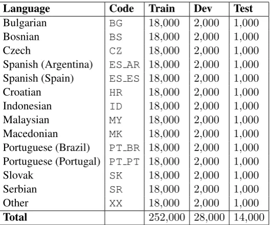
Table 1: The languages included in the corpus and the number of sentences in each set.

3 Data

The data for the shared task comes from the DSL Corpus Collection (Tan et al., 2014). The task is performed at the sentence-level and the corpus consists of 294,000 sentences distributed evenly between14language classes. The corpus is subdi-vided into training, development and test sets. The languages and the number of sentences in each set are listed in Table 1.

An interesting addition to this year’s data is the inclusion of an “other” class which contains data from various additional languages. The motiva-tion here is to emulate a realistic language identi-fication and see how the systems perform in clas-sifying previously unseen languages.

More details about the data can be found in the shared task overview paper (Zampieri et al., 2015).

4 Method

In this section we describe the general methodol-ogy used to construct our system. We use a super-vised learning approach based on discriminative classifiers.

4.1 Features

We use two basic classes of surface features: char-actern-grams (n= 1–6) and wordn-grams (n= 1–2).

4.2 Classifier

We use a linear Support Vector Machine to per-form multi-class classification in our experiments.

In particular, we use the LIBLINEAR2 _package (Fan et al., 2008) which has been shown to be effi-cient for text classification problems such as this. For example, it has been demonstrated to be a very effective classifier for the task of Native Language Identification (Malmasi and Dras, 2015b; Malmasi et al., 2013) which also relies on text classification methods.

5 Classifier Ensembles

Classifier ensembles are a way of combining dif-ferent classifiers or experts with the goal of im-proving accuracy through enhanced decision mak-ing. They have been applied to a wide range of real-world problems and shown to achieve better results compared to single-classifier methods (Oza and Tumer, 2008). Through aggregating the puts of multiple classifiers in some way, their out-puts are generally considered to be more robust. Ensemble methods continue to receive increasing attention from researchers and remain a focus of much machine learning research (Wo´zniak et al., 2014; Kuncheva and Rodr´ıguez, 2014).

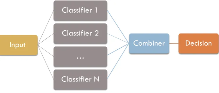
Such ensemble-based systems often use a par-allel architecture, as illustrated in Figure 1, where the classifiers are run independently and their out-puts are aggregated using a fusion method. Other, more sophisticated, ensemble methods that rely on meta-learning may employ a stacked architecture where the output from a first set of classifiers is fed into a second level meta-classifier and so on.

Input

Classifier 1

Classifier 2

Combiner

Decision

…

Classifier N

Ensemble Architecture

2

Figure 1: An example of parallel classifier ensemble architecture whereN independent classifiers pro-vide predictions which are then fused using an ensemble combination method.

The first part of creating an ensemble is gen-erating the individual classifiers. Various meth-ods for creating these ensemble elements have been proposed. These involve using different al-gorithms, parameters or feature types; applying different preprocessing or feature scaling meth-ods and varying (e.g.distorting or resampling) the training data.

For example, Bagging (bootstrap aggregating) is a commonly used method for ensemble genera-tion (Breiman, 1996) that can create multiple base classifiers. It works by creating multiple boot-strap training sets from the original training data and a separate classifier is trained from each one of these sets. The generated classifiers are said to be diverse because each training set is created by sampling with replacement and contains a random subset of the original data.Boosting(e.g.with the AdaBoost algorithm) is another method where the base models are created with different weight dis-tributions over the training data with the aim of assigning higher weights to training instances that are misclassified (Freund and Schapire, 1996).

As we describe in section 7, each of the base classifiers in our ensemble is trained on a different feature space, as this has proven to be effective.

The second part of ensemble design is choosing a fusion rule to aggregate the outputs from the var-ious learners, this is discussed in the next section.

6 Ensemble Combination Methods

Once it has been decided how the set of base clas-sifiers will be generated, selecting the classifier combination method is the next fundamental de-sign question in ensemble construction.

The answer to this question depends on what output is available from the individual classifiers. Some combination methods are designed to work with class labels, assuming that each learner out-puts a single class label prediction for each data point. Other methods are designed to work with class-based continuous output, requiring that for each instance every classifier provides a measure of confidence probability3 _{for each class label.} These outputs for each class usually sum to1over all the classes.

Although a number of different fusion methods have been proposed and tested, there is no sin-gle dominant method (Polikar, 2006). The perfor-mance of these methods is influenced by the nature of the problem and available training data, the size of the ensemble, the base classifiers used and the diversity between their outputs.

The selection of this method is often done em-pirically. Many researchers have compared and contrasted the performance of combiners on dif-ferent problems, and most of these studies – both empirical and theoretical – do not reach a defini-tive conclusion (Kuncheva, 2014, p 178).

In the same spirit, we experiment with sev-eral information fusion methods which have been widely discussed in the machine learning litera-ture. Our selected methods are listed below. Var-ious other methods exist and the interested reader can refer to the exposition by Polikar (2006).

3_{i.e.an estimate of the posterior probability for the label.}

6.1 Plurality voting

Each classifier votes for a single class label. The votes are tallied and the label with the highest number4_{of votes wins. Ties are broken arbitrarily.} This voting method is very simple and does not have any parameters to tune. An extensive analy-sis of this method and its theoretical underpinnings can be found in the work of (Kuncheva, 2004, p. 112).

6.2 Mean Probability Rule

The probability estimates for each class are added together and the class label with the highest aver-age probability is the winner. This is equivalent to the probability sum combiner which does not re-quire calculating the average for each class. An important aspect of using probability outputs in this way is that a classifier’s support for the true class label is taken in to account, even when it is not the predicted label (e.g.it could have the sec-ond highest probability). This method has been shown to work well on a wide range of problems and, in general, it is considered to be simple, intu-itive, stable (Kuncheva, 2014, p. 155) and resilient to estimation errors (Kittler et al., 1998) making it one of the most robust combiners discussed in the literature.

6.3 Median Probability Rule

Given that the mean probability used in the above rule is sensitive to outliers, an alternative is to use the median as a more robust estimate of the mean (Kittler et al., 1998). Under this rule each class label’s estimates are sorted and the median value is selected as the final score for that label. The label with the highest median value is picked as the winner. As with the mean combiner, this method measures the central tendency of support for each label as a means of reaching a consensus decision.

6.4 Product Rule

For each class label, all of the probability esti-mates are multiplied together to create the label’s final estimate (Polikar, 2006, p. 37). The label with the highest estimate is selected. This rule can provide the best overall estimate of posterior probability for a label, given that the individual es-timates are accurate. A trade-off here is that this

4_{This differs with amajorityvoting combiner where a}

la-bel must obtain over50%of the votes to win. However, the names are sometimes used interchangeably.

NONTRAINABLE (FIXED) COMBINATION RULES 151

Decision profile COMBINER Class label MAX D1 D₂ … Feature vector Classifiers DL AVERAGE

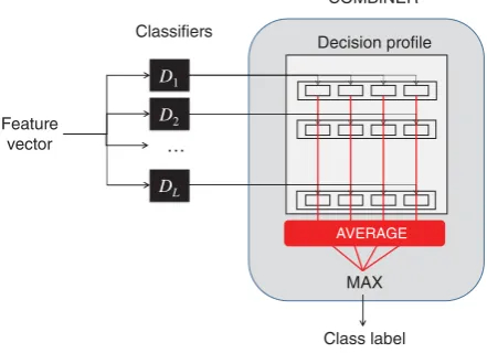
FIGURE 5.5 Operation of the average combiner.

Represented by the average combiner, the category of simple nontrainable combiners is described in Figure 5.4, and illustrated diagrammatically in Figure 5.5. These combiners are called nontrainable, because once the individual classifiers are trained, their outputs can be fused to produce an ensemble decision, without any further training.

◻◼ Example 5.3 Simple nontrainable combiners

The following example helps to clarify simple combiners. Let c=3 and L=5. Assume that for a certainx

DP(x)= ⎡ ⎢ ⎢ ⎢ ⎢ ⎣

0.1 0.5 0.4 0.0 0.0 1.0 0.4 0.3 0.4 0.2 0.7 0.1 0.1 0.8 0.2

⎤ ⎥ ⎥ ⎥ ⎥ ⎦ . (5.20)

Applying the simple combiners column wise, we obtain:

Combiner 𝜇1(x) 𝜇2(x) 𝜇3(x)

Average 0.16 0.46 0.42 Minimum 0.00 0.00 0.10 Maximum 0.40 0.80 1.00 Median 0.10 0.50 0.40 40% trimmed mean 0.13 0.50 0.33 Product 0.00 0.00 0.0032 Figure 2: An example of a mean probability com-biner. The feature vector for a sample is input toL different classifiers, each of which output a vec-tor of confidence probabilities for each possible class label. These vectors are combined to form the decision profile for the instance which is used to calculate the average support given to each la-bel. The label with the maximum support is then chosen as the prediction. Image reproduced from (Kuncheva, 2014).

method is very sensitive to low probabilities: a sin-gle low score for a label from any classifier will essentially eliminate that class label.

6.5 Highest Confidence

In this simple method, the class label that receives the vote with the largest degree of confidence is selected as the final prediction (Kuncheva, 2014, p. 150). In contrast to the previous methods, this combiner disregards the consensus opinion and in-stead picks the prediction of the expert with the highest degree of confidence.

6.6 Borda Count

This method works by using each classifier’s con-fidence estimates to create a ranked list of the class labels in order of preference, with the predicted label at rank 1. The winning label is then se-lected using the Borda count5_{algorithm (Ho et al.,} 1994). The algorithm works by assigning points to labels based on their ranks. If there areN dif-ferent labels, then each classifiers’ preferences are assigned points as follows: the top-ranked label receivesN points, the second place label receives

5_{This method is generally attributed to Jean-Charles de}

N −1 points, third place receivesN −2points and so on with the last preference receiving a sin-gle point. These points are then tallied to select the winner with the highest score.

The most obvious advantage of this method is that it takes into account each classifier’s prefer-ences, making it possible for a label to win even if another label received the majority of the first preference votes.

6.7 Oracle

We use an “Oracle” combiner as one possible ap-proach to estimating the upper-bound for classifi-cation accuracy. This method has previously been used to analyze the limits of majority vote clas-sifier combination (Kuncheva et al., 2001). The oracle will assign the correct class label for an in-stance if at least one of the constituent classifiers in the ensemble produces the correct label for that data point. Oracles are usually used in compara-tive experiments and to gauge the performance and diversity of the classifiers chosen for an ensemble (Kuncheva, 2002; Kuncheva et al., 2003). They can help us quantify the potential upper limit of an ensemble’s performance on the given data and how this performance varies with different ensem-ble configurations (Malmasi et al., 2015b).

7 Systems

We test three different systems in our submissions to the shared task, as outlined here.

7.1 System 1

We train a single model based on a simple combi-nation of all our feature types into a single feature space. The model has approximately13.6million features. This was the first system that we built and it achieved very good results of94-95% dur-ing testdur-ing. It was selected as our first submission.

7.2 System 2

The second system is an ensemble classifier, as de-scribed in section 5. The aim here was to improve over the single classifier system described in sec-tion 7.1. Each base classifier in the ensemble is trained on a separate feature type, resulting in a total of eight classifiers in the system.

During the development of our system we tested the six ensemble fusion methods described in sec-tion 6. Our experiments with the training and de-velopment data showed that the mean probability combiner yielded the best accuracy.

We achieved an accuracy of 95.5% on the de-velopment set against an oracle accuracy of99%, showing that the combiner was very close to the upper-bound of possible classification accuracy. This result was slightly better than that of Sys-tem 1, so this method was selected for our second submission. The results from the other combiners were also in a similar range, but we used the mean probability combiner for our second system.

7.3 System 3

Our final system is identical to the second system in its method and setup with the exception that some weak and redundant features were removed. We suspected that there may be some redundancy in the large number of charactern-gram features and removing these might increase the diversity, and thus accuracy, of the ensemble.

Using the feature analysis methodology out-lined by Malmasi and Cahill (2015), we analyzed the feature interactions using the training and de-velopment sets. This methodology uses Yule’s Q-coefficient statistic (Yule, 1912), which can be a useful measure of pairwise dependence between two classifiers (Kuncheva et al., 2003). This no-tion of dependence relates to complementarity and orthogonality, and is an important factor in com-bining classifiers (Lam, 2000). The calculated Q-coefficient ranges between −1 to +1, where −1

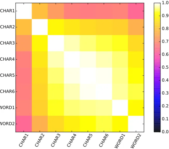
signifies negative association, 0 indicates no as-sociation (independence) and +1 means perfect positive correlation (dependence). We apply this method to our ensemble to calculate the depen-dence between the classifiers. The results for the analysis are shown as a heat map in Figure 3.

We see that the predictions obtained using char-acter unigrams are very diverse to the other fea-tures, as noted by the low Q-coefficient. This di-versity is a result of character unigrams being a weak feature: they only achieve around 76% ac-curacy whereas most other feature types can ob-tain>90%accuracy. As a result we removed this feature from the ensemble.

CHAR1 CHAR2 CHAR3 CHAR4 CHAR5 CHAR6 _{WORD1 WORD2}

CHAR1

CHAR2

CHAR3

CHAR4

CHAR5

CHAR6

WORD1

WORD2

0.0 0.1 0.2 0.3 0.4 0.5 0.6 0.7 0.8 0.9 1.0

Figure 3: The matrix of pairwise Q-coefficient values between our feature types, displayed as a heat map. Smaller values indicate lower dependence between their predictions.

Normal NE Removed Rank Accuracy Rank Accuracy

Random Baseline — 7.14% — 7.14% System 1 3 95.31% 2 93.88% System 2 2 95.44% 3 93.73% System 3 1 95.54% 1 94.01%

Table 2: Results for our three system on the test set. The accuracy and rank among all systems in the shared task are shown. Our optimized ensem-ble ranked first in both tasks.

To recap, our third system is a modification of the second system where we remove character1-,

3- and 5-grams in order to increase the ensemble diversity. This reduced ensemble was chosen as our third submission as it achieved slightly higher results than the full ensemble during development.

8 Results

We entered our systems in both sub-tasks of the closed training track. We did not enter the open training track of the competition. The first sub-task (the “normal” sub-task) required our system to classify 14,000 unlabelled sentences. The sec-ond task was also similar, but it used a different set of sentences which also had all named entities (NE) removed (“NE Removed” task). This is

be-cause it is assumed that features related to NEs can strongly influence the results.

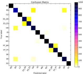
Our systems took the top three places for both subtasks. The results and rankings for each system are shown in Table 2. We note that System 3 — the optimized ensemble — was the winning entry for both tasks. This comports with our initial tests where it was our best system during development. The confusion matrix for our best results in the normal task are shown in Figure 4. We achieved a perfect 100%accuracy for four classes: Czech (CZ), Macedonian (MK), Slovak (SK) and Other (XX). Bulgarian (BG) was also close with only a single sentence being misclassified as Macedo-nian. These results suggest that confusion between Bulgarian–Macedonian and Czech–Slovak is not a significant issue here. The greatest confusion is between the Bosnian–Croatian–Serbian6_{group as} well as the Spanish and Portuguese dialect pairs. Bosnian is the worst performing language among the14classes.

We also analyze the learning rate for the fea-tures in our system. The cross-validation accu-racy for four different feature types is shown in Figure 5. Higher order character n-grams seem to outperform wordn-grams. Word bigrams are lower in accuracy and have a steeper learning rate.

6_{We also observe that Bosnian is the most confused class}

BG BS CZ

ES_AR ES_ES HR ID MK MY PT_BR PT_PT SK SR XX

Predicted label BG

BS CZ ES_AR ES_ES HR ID MK MY PT_BR PT_PT SK SR XX

True label

Confusion Matrix

0 100 200 300 400 500 600 700 800 900 1000

Figure 4: The confusion matrix for our results on the test set (normal task).

0 50000 100000 150000 200000 250000 300000 Training examples

0.84 0.86 0.88 0.90 0.92 0.94 0.96

Accuracy

Learning Curves

Character 3-grams Character 5-grams Word unigrams Word bigrams

Figure 5: Learning curves for some of our features based on cross-validation accuracy. We observe that charactern-grams perform better than word-based n-grams. The accuracy does not plateau with the entire training data used.

We also observe that accuracy increases contin-uously as the training data is increased. This sug-gests that despite the already large size of the train-ing set, there is still room for further improvement by adding more data. However, this would also re-sult in an increase in the size of our feature space, which is already quite large due to the prodigious growth rate of the larger order charactern-grams.

9 Discussion and Conclusion

In this work we demonstrated the utility of clas-sifier ensembles for text classification. Using an ensemble composed of base classifiers trained on character 1–6 grams and word unigrams and bi-grams, we were able to outperform the other en-tries in the closed track of the DSL 2015 shared task.

A crucial direction for future work is the investi-gation of methods to reduce the confusion between these three groups of classes.

In this work we did not experiment with fea-ture selection methods to evaluate if this can fur-ther enhance performance, or at least efficiency by reducing the dimensionality of the feature space. One weakness of our system may be the very high dimensionality of the feature space with almost14

million features. Having such a large number of features can be inefficient and may impede the use of our system for real-time applications.

References

Kenneth R Beesley. 1988. Language identifier: A computer program for automatic natural-language identification of on-line text. InProceedings of the 29th Annual Conference of the American Transla-tors Association, volume 47, page 54. Citeseer.

Leo Breiman. 1996. Bagging predictors. InMachine Learning, pages 123–140.

William B. Cavnar and John M. Trenkle. 1994. N-Gram-Based Text Categorization. In Proceedings of SDAIR-94, 3rd Annual Symposium on Document Analysis and Information Retrieval, pages 161–175, Las Vegas, US.

Ted Dunning. 1994. Statistical identification of lan-guage. Computing Research Laboratory, New Mex-ico State University.

Rong-En Fan, Kai-Wei Chang, Cho-Jui Hsieh, Xiang-Rui Wang, and Chih-Jen Lin. 2008. LIBLINEAR: A Library for Large Linear Classification. Journal of Machine Learning Research, 9:1871–1874.

Yoav Freund and Robert E Schapire. 1996. Exper-iments with a new boosting algorithm. In ICML, volume 96, pages 148–156.

Tin Kam Ho, Jonathan J. Hull, and Sargur N. Srihari. 1994. Decision combination in multiple classifier systems. Pattern Analysis and Machine Intelligence, IEEE Transactions on, 16(1):66–75.

Chu-Ren Huang and Lung-Hao Lee. 2008. Contrastive Approach towards Text Source Classification based on Top-Bag-Word Similarity.

Josef Kittler, Mohamad Hatef, Robert PW Duin, and Jiri Matas. 1998. On combining classifiers. IEEE Transactions on Pattern Analysis and Machine In-telligence, 20(3):226–239.

Ludmila I Kuncheva and Juan J Rodr´ıguez. 2014. A weighted voting framework for classifiers en-sembles. Knowledge and Information Systems, 38(2):259–275.

Ludmila I Kuncheva, James C Bezdek, and Robert PW Duin. 2001. Decision templates for multiple clas-sifier fusion: an experimental comparison. Pattern Recognition, 34(2):299–314.

Ludmila I Kuncheva, Christopher J Whitaker, Cather-ine A Shipp, and Robert PW Duin. 2003. Limits on the majority vote accuracy in classifier fusion. Pat-tern Analysis & Applications, 6(1):22–31.

Ludmila I Kuncheva. 2002. A theoretical study on six classifier fusion strategies. IEEE Transac-tions on pattern analysis and machine intelligence, 24(2):281–286.

Ludmila I Kuncheva. 2004. Combining Pattern Clas-sifiers: Methods and Algorithms. John Wiley & Sons.

Ludmila I Kuncheva. 2014. Combining Pattern Clas-sifiers: Methods and Algorithms. Wiley, second edi-tion.

Louisa Lam. 2000. Classifier combinations: imple-mentations and theoretical issues. InMultiple clas-sifier systems, pages 77–86. Springer.

Nikola Ljubesic, Nives Mikelic, and Damir Boras. 2007. Language indentification: How to distinguish similar languages? InInformation Technology In-terfaces, 2007. ITI 2007. 29th International Confer-ence on, pages 541–546. IEEE.

Shervin Malmasi and Aoife Cahill. 2015. Measuring Feature Diversity in Native Language Identification. InProceedings of the Tenth Workshop on Innovative Use of NLP for Building Educational Applications, Denver, Colorado, June. Association for Computa-tional Linguistics.

Shervin Malmasi and Mark Dras. 2015a. Automatic Language Identification for Persian and Dari texts. In Proceedings of the 14th Conference of the Pa-cific Association for Computational Linguistics (PA-CLING 2015), pages 59–64, Bali, Indonesia, May.

Shervin Malmasi and Mark Dras. 2015b. Large-scale Native Language Identification with Cross-Corpus Evaluation. In Proceedings of NAACL-HLT 2015, Denver, Colorado, June. Association for Computa-tional Linguistics.

Shervin Malmasi, Sze-Meng Jojo Wong, and Mark Dras. 2013. NLI Shared Task 2013: MQ Submis-sion. InProceedings of the Eighth Workshop on In-novative Use of NLP for Building Educational Ap-plications, pages 124–133, Atlanta, Georgia, June. Association for Computational Linguistics.

Shervin Malmasi, Eshrag Refaee, and Mark Dras. 2015a. Arabic Dialect Identification using a Parallel Multidialectal Corpus. In Proceedings of the 14th Conference of the Pacific Association for Computa-tional Linguistics (PACLING 2015), pages 209–217, Bali, Indonesia, May.

Shervin Malmasi, Joel Tetreault, and Mark Dras. 2015b. Oracle and Human Baselines for Native Lan-guage Identification. In Proceedings of the Tenth Workshop on Innovative Use of NLP for Building Educational Applications, Denver, Colorado, June. Association for Computational Linguistics.

Nikunj C Oza and Kagan Tumer. 2008. Classifier en-sembles: Select real-world applications. Informa-tion Fusion, 9(1):4–20.

Liling Tan, Marcos Zampieri, Nikola Ljubeˇsic, and J¨org Tiedemann. 2014. Merging comparable data sources for the discrimination of similar languages: The dsl corpus collection. InProceedings of the 7th Workshop on Building and Using Comparable Cor-pora, pages 11–15, Reykjavik, Iceland.

J¨org Tiedemann and Nikola Ljubeˇsi´c. 2012. Efficient discrimination between closely related languages. InProceedings of COLING 2012, pages 2619–2634. Michał Wo´zniak, Manuel Gra˜na, and Emilio Corchado. 2014. A survey of multiple classifier systems as hy-brid systems. Information Fusion, 16:3–17. George Udny Yule. 1912. On the methods of

measur-ing association between two attributes. Journal of the Royal Statistical Society, pages 579–652. Marcos Zampieri and Binyam Gebrekidan Gebre.

2012. Automatic identification of language vari-eties: The case of Portuguese. In KONVENS2012-The 11th Conference on Natural Language Process-ing, pages 233–237. ¨Osterreichischen Gesellschaft f¨ur Artificial Intelligende ( ¨OGAI).

Marcos Zampieri, Binyam Gebrekidan Gebre, and Sascha Diwersy. 2013. N-gram language models and POS distribution for the identification of Span-ish varieties. InProceedings of TALN 2013, pages 580–587.

Marcos Zampieri, Liling Tan, Nikola Ljubeˇsic, and J¨org Tiedemann. 2014. A report on the DSL shared task 2014. COLING 2014, page 58.