General correcting formulae for forecasts

Munich Personal RePEc Archive

General correcting formulae for forecasts

Harin, Alexander

Modern University for the Humanities

12 April 2014

1

General correcting formulae for forecasts

Alexander Harin

aaharin@yandex.ru

Modern University for the Humanities

The concept of unforeseen events is considered as a part of a hypothesis of uncertain future. The applications of the consequences of the hypothesis in utility and prospect theories are reviewed. Partially unforeseen events and their role in forecasting are analyzed. Preliminary preparations are shown to be able, under specified conditions, to quicken the revisions of forecasts and to hedge or diversify financial risks after partially unforeseen events have occurred. General correcting formulae for forecasts are proposed.

Keywords: forecast, uncertainty, risk, utility, Ellsberg paradox,

Contents

Introduction ……… 2

Prehistory of the research An example. Hiroshima 1945

1. Preliminary considerations ……….. 4

1.1. Partially unforeseen events

1.2. About the continuity and differentiability of approximations 1.3. On the validity of the approximation forecasting.

1.4. Frames of reference and transformations

1.5. The piecewise smooth representation

for univariate and multivariate models

2. Particular formulae for univariate models ………. 7

2.1. General notes

2.2. Low-order approximations by sub-functions

2.3. Additive-multiplicative formulae

2.4. Transformations

3. Applications ……….. 11

3.1. Unforeseen events. Forecasts, perspectives and plans

3.2. New resources and areas

4. Unforeseen events and a hypothesis of uncertain future ……… 14

4.1. Unforeseen events and the hypothesis

4.2. Illustrating examples and applications

Conclusions ……… 31

2

Introduction

Prehistory of the research

An absolutely exact knowledge is one of main aims of science. Surely, in many cases it can be attained for the past. But can it be attained for the future? Can forecasts be absolutely exact?

Many works have been devoted to accuracy and errors of forecasts (see, e.g., Chang, 2011, Morlidge, 2013, McAleer, 2008), including the influence of unforeseen, unanticipated events (see, e.g., Hendry and Mizon, 2013). There are works those analyze breaks and news impact surfaces (see., e.g., Clements and Hendry, 2006, Caporin and McAleer, 2011, Castle et al, 2012).

The unforeseen events can be either of the natural character as earthquakes or due to human activity. The possibilities of humankind technical power and technologies grow faster and faster. Due to this tendence, scientific discoveries, inventions and innovations become the growing sources of unforeseen events.

This article is devoted to partially unforeseen events and their influence on forecasting.

The considerations and formulae of the article can be used in various fields of human activity, including pure and applied science, economics and business, risk management, measuring the implicit risks, hedging financial risks, computing "capital charges that are required to cover unforeseen and extreme financial market fluctuations" (see Caporin and McAleer, 2010).

The importance of unforeseen events and partially unforeseen events cannot be overestimated. The unforeseen events can crucially and, sometimes, dramatically change situations. The "black swans" are an example of them. This work serves to smooth down or even turn to advantage the consequences of such events.

3

An example. Hiroshima 1945

Let us suppose, that in 1930-35, an imaginary estimate of risk was needed with respect to bombing for an underground factory, government bomb-proof shelter, etc. for the year 1945. Suppose, in 1930-35 the ideal forecast was made. The forecast should be based firstly, e.g., on the forecast of the maximal power of an aircraft bomb for 1945. The forecast should be based secondly, e.g., on the maximal weight that bombing aircraft can lift.

To 1945, due to the most optimistic forecasts, a bombing aircraft could lift a bombing weight much less than 20 tons and even less when calculating in trinitrotoluene equivalent. In 1945 Hiroshima was bombed by the 4-tons atomic bomb. But it was equal to 20000 tons in trinitrotoluene equivalent. So, the initial estimate of risk was catastrophically wrong.

The prerequisite of an atomic bomb (the division of uranium) was discovered in 1938. Naturally, in 1930-35 it was an unforeseen event. So, in this case the relative error, caused by the unforeseen event, is more than 1000 (more than 100000%).

4

1. Preliminary considerations

1.1. Partially unforeseen events

There is a wealth of sorts of unforeseen events. According to Caporin and McAleer (2010) these events may be represented by univariate and multivariate models depending on the numbers of the events. We may divide them also into two types: fully unforeseen events and partially unforeseen events.

Rigorously speaking, in the presence of fully unforeseen events, we cannot make any reliable forecast. In other words, "If anything can happen, then nothing can be predicted."

Let us consider further the partially unforeseen events.

1.2. About the continuity and differentiability of approximations

When choosing an adequately detailed time scale, the vast majority of macro-world phenomena are characterized by continuity in time. The discontinuity, the discreteness in time is observed only in quantum phenomena, for example at the birth of elementary particles. Therefore, the description of the phenomena of the macro-world by means of continuous functions is lawful.

Changes in the macro-world phenomena, that is, the acceleration in a particular dimension, requires physical movements, changes of electromagnetic fields, etc. That is, they are also characterized by continuity in time. Therefore, the description of differentiable functions is lawful for the description of the macro-world phenomena.

1.3. On the validity of the approximation forecasting

As for the macro-world phenomena the description by differentiable functions is lawful, then the forecasts of these phenomena in the form of approximations is lawful also. In this sense we can say that the future is a continuation of the present. And we can do calculations and estimates for the prediction of future events of macro-world on the basis of data on current status and rate of change of these phenomena. Naturally, accurate calculations are possible only for sufficiently small time intervals for which this approximation is correct. But an approximation approach is possible for longer intervals of time, as the basis for assessing the possible deviations.

5

1.4. Frames of reference and transformations

From physics it is well known an event may be described in various frames of reference. Optimal choice of frame of reference is well known to be valuable. When one use various frames of reference, the expressions of transmission between various frames of reference are necessary.

Suppose a wheel rolls along the road. We should calculate the trajectory of a point of the rim. It is the cycloid which is a complex transcendental curve. But if we choose the frame of reference in the center of the rim, we obtain two simple trajectories: the trajectory of the center of the rim and the circular trajectory of the point of the rim around the rim.

Suppose a firm has a property, pays profit tax, pays turnover tax and speculates on the stock-exchange. If we do not know nothing about the firm except its total capital, then the dependence of the capital on the time is complex and obscure, incomprehensible. If we know the time points and the bases of the operations of the firm, then the dependence may be represented as the sum of the simple elementary dependences.

1.5. The piecewise smooth representation for univariate and multivariate models

Let us consider a pure mathematical case of infinitely differentiable analytical forecast functions. Consider a function F(t) : F(t) is infinitely differentiable and analytic in a point tBase of the timeline and on the semi-closed interval [tBase, t).

Let us denote the Taylor series of the forecast function F(t) as F(tBase, t)

∑

=

− +

=

1 ) (

) (

! ) ( )

( ) , (

n

n Base Base

n

Base

Base t t

n t F t

F t t

F .

where F(n)(tBase) is the n-th derivative of F(t) in the point tBase.

Suppose there is a rupture of an n-th : n≥1, derivative of F(t) in the point

tCorr,1≡t1: tBase<t1<t, (tCorr,0≡t0≡tBase), but F(t) is infinitely differentiable and

analytic on (tCorr,1, t). Then, for univariate models, we obtain

∑

=

− +

=

1

1 , 1

, ) (

1 , 1

, ( )

! ) ( )

( ) , (

n

n Corr Corr

n

Corr

Corr t t

n t F t

F t t

F .

6

By means of the identical transformation we obtain for F(t)

)] , ( ) , ( [ ) , ( )] , ( ) , ( [ ) , ( ) , ( ) , ( ) , ( ) , ( ) ( 0 1 0 1 , 1 , 1 , t t F t t F t t F t t F t t F t t F t t F t t F t t F t t F t F Base Corr Base Base Base Corr Corr − + ≡ − + = − + ≡ = .

Denoting the modification of the function ΔF(tCorr,r-1, tCorr,r, t)≡[F(tCorr,r, t)-F(t Corr,r-1, t)], we have

) , , ( ) , ( )

(t F t t F t t ,1 t

F = Base +∆ Base Corr .

For R : R<∞, rupture points tr:tBase≡t0, tr-1<tr<t : 1≤r≤R, (see also Castle et al,

2012) we obtain the general piecewise smooth representation for multivariate models

∑

r t t

t F t t F t F 1 1 0, ) ( , , )

( )

( .

Suppose a set of sub-functions {f1r(tr-1, tr, t), …, fsr(tr-1, tr, t), …, fSr(tr-1, tr, t)}≡{fsr(tr-1, tr, t)} : S<∞, fsr(tr-1, tr, tr)=0, of the modification of the function ΔF(t r-1, tr, t) exists such as ΔF(tr-1, tr, t) may be represented as ΔF(tr-1, tr, t)=ΔF({fsr(tr-1, tr, t)}) and ΔF({fsr(tr-1, tr, t)}) is infinitely differentiable with respect to any fsr(tr-1, tr, t) and analytic on ({fsr(tr-1, tr, tr)}, {fsr(tr-1, tr, t)}]. Let us denote a differential

operator ) , , ( ) , , ( ... ) , , ( ) , , ( 1 1 1 1 1 1 t t t f t t t f t t t f t t t f T r r Sr r r Sr r r r r r r − − − − _∂ ∂ + + ∂ ∂ = ,

where the derivatives are the right-side limits in the point tr. Then we have

∑

7

2. Particular formulae for univariate models

2.1. General notes

Let us further consider the case of the only rupture point, of the point of correction t1≡tCorr,1≡tCorr

) , , ( ) , ( )

(t F t t F t t t F = Base +∆ Base Corr .

Probably, the simplest sorts of partially unforeseen events are those having only unforeseen point of time or unforeseen magnitude and being represented by univariate models. Let us consider them further.

Let us suppose a partially unforeseen event with an unforeseen magnitude and/or an unforeseen point of time has taken place at tCorr.

If we know the unit value δ1F(tr-1, tr, t) of modification of the function, which

corresponds to the unit magnitude of the event, and if at t>tCorr we know the point

of time tCorr and we may determine the magnitude M, then we may denote ΔF(tr-1, tr, t)≡M*δ1F(tr-1, tr, t).

If we have known the correction time point tCorr, then we may express the

modification of the function F(t) also.

So, for the partially unforeseen events with the unforeseen magnitude and point of time, we may remain the form of the expression unchanged.

From physics it is well known an event may be described in various frames of reference. Optimal choice of frame of reference is well known to be valuable. When one use various frames of reference, the expressions of transformations between various frames of reference are necessary.

2.2. Low-order approximations by sub-functions

If a rupture of an n-th (where n≥1) derivative of F(n)(t) in a point tCorr is

caused by a foreseen event, then the series of the right-hand limits of the derivatives

F(n)(tCorr) may be calculated in advance and the forecast may be corrected in

advance also. If this rupture is caused by an unforeseen event, then sometimes the forecast correction should be performed extremely rapidly.

Let us consider a case of two preliminary conditions:

1) The calculation of the right-hand limits of the derivatives F(n)(tCorr) (or the

explicit calculation of F(t)) is very complicated and needs too long time to be

admissible.

2) The function F(t) may be represented by means of a finite set of sub-functions fs(t) as

)}) ( ({ )}) ( ),..., ( ({ )

(t F f₁ t f t F f t

F = S ≡ s .

and the derivatives

n k

s n

t f

t f F

)) ( (

)}) ( ({

∂ ∂

of ΔF or F may be calculated in advance.

8 3. The derivatives

n k s n t f t f F )) ( ( )}) ( ({ ∂ ∂

are happened to do not essentially depend on this partially unforeseen event and the preliminarily calculated derivatives may be used (or they may be corrected during the admissible time).

Let us suppose, that the first few L terms give sufficient accuracy of

approximation. Then Error L l Corr Corr Base p l n n Base Base n Base l t t t f F T t t n t F t F t F ∆ ± ∆ + − + ≈

∑

∑

where ΔError is the total error. Note, that ΔError+ errors can essentially differ from

ΔError-. The impact of negative shocks can differ from that of positive shocks (see,

e.g., Caporin and McAleer 2011).

For the first order approximation, the general formula may be easily simplified to Error S k Corr Corr Base k Corr Base k Corr Base s t n n Base Base n Base t t t f t t f t t f F t t n t F t F t F Corr ∆ ± ∂ ∆ ∂ + − + ≈

∑

∑

It may be expressed also as the derivative of a complex function

9

2.3. Additive-multiplicative formulae

Let us suppose that the modification of the forecast function ΔF(tBase, tCorr t)

of an object may be exactly or approximately expressed in the form of explicit functions. These functions may be internal (relative to the object), external (relative to the object), periodic, etc, to specialize, specify unified and standardized forecasts to special, specific forecasting objects and situations. Then the modification ΔF(tBase, tCorr t) may be written in a general form as, for example,

) }, ) , , ( { }, ) , , ( { }, ) , , ( { }, ) , , ( ({ ) , , ( , , , , Error Corr m Special Corr l Periodic Corr k External Corr i Internal Corr Corr Base Corr t t f t t f t t f t t f F t t t F ∆ ∆ ≈ ∆ .

where and further:

{finternal,i} - the set of internal (relative to the object) functions; {fexternal,k} - the set of external (relative to the object) functions. {fperiodic,l} - the set of periodic functions;

{fspecial,m} - the set of specializing, specifying, adapting, concretizing functions to

specialize, specify unified and standardized forecasts to special, specific forecasting objects and situations.

The operations of addition and multiplication are, probably, the most common and important ones as in practice so in the pure mathematics (see, e.g., Waerden van der, 1976).

Let us suppose that the partially unforeseen modification of the forecast function ΔF(tBase, tCorr t) may be exactly or approximately expressed by means of

additive and multiplicative functions. Here, an additive function implies a function which additively contributes to the forecast. Here, a multiplicative function implies a function which additively contributes to the forecast.

Let us consider, as a heuristic hypothesis, the following formula

] 1 [ ] ) , ( ) , ( ) , ( [ ) , , ( 1 , 1 , Error A a Corr a Addit M m Corr m t Multiplica Base Base Corr Base t t t t K t t F t t t F ∆ ± × Φ + × ≈

∑

∏

or, omitting the variables and indices,

] 1

[ ]

[FBase KMultiplicat Addit Error

F ≈ ×

∏

∑

where and further:

F(tBase, tCorr, t) - the corrected forecast for the moment t; FBase(tBase, t) - the base forecast for the moment t;

∏KMultiplicat,m - the product from 1 to M of the multiplicative (absolute)

functions (coefficients) for partially unforeseen corrections; ∑ФAddit,a - the sum from 1 to A of the additive (absolute) fu

10 For the cases when

0 ) , ( ) , ( 1 , ≠ ×

∏

Base t t K t t

F ,

(preferentially for F~Fbase) this formula may be written as

] 1 [ )] , ( 1 [ ] )) , ( 1 ( [ ) , ( ) , , ( 1 , 1 , Error A a Corr a Addit M m Corr i t Multiplica Base Base Corr Base t t t t k t t F t t t F ∆ ± × + × + × ≈

∑

∏

or, omitting the variables and indices,

] 1 [ ] 1 [ )] 1 (

[ _{Multiplicat Addit Error}

Base k

F

F ≈ ×

∏

∑

where and further:

∏(1+kMultiplicat,m) - the product from 1 to M of the multiplicative (relative)

functions (coefficients) for partially unforeseen corrections;

∑φAddit,a - the sum from 1 to A of the additive (relative) functions

(normalized on FBase×∏KMultiplicat,m) for partially unforeseen (absolute) corrections.

2.4. Transformations

We may easily obtain the transformations between the versions of the formula.

For the multiplicative functions

m t Multiplica m t Multiplica k

K , =1+ , .

For the additive functions

∏

Addit F k

1

, ,

11

3. Applications

3.1. Unforeseen events. Forecasts, perspectives and plans

Perspectives can be determined, ascertained by forecasts and estimates. Perspectives are guidelines for plans. The concept of unforeseen events and the hypothesis of uncertain future can put some questions about forecasts, perspectives and plans.

Let us remind that the first consequence of the hypothesis of uncertain future means that unforeseen events can occur. The second consequence of the hypothesis of uncertain future means that the greater the data dispersion (uncertainty), the smaller the probability of a future event near the probability p~1, and the greater can be the probability of a future event near the probability p~0.

Further, the terms short-term, medium-term, long-term and super long-term forecasting and planning will be sufficiently conditional and will be treated mainly with respect to the forecasting time intervals and changes of the projected objects.

Forecasts

Possibility of absolutely accurate forecasting. A question follows from the second consequence of the hypothesis of uncertain future: Is an absolutely accurate (and reasonably reliable) forecast possible?

Possibility of absolutely reliable forecasting. A question follows from the second consequence of the hypothesis of uncertain future: Is an absolutely reliable (reasonably accurate) forecast possible?

Possibility of mid-term quantitative forecasting. The term "the quantitative forecasting" will mean the accuracy of the forecasting not worse than, for example, 20% -30%. A question follows from the first consequence of the hypothesis of uncertain future: Is a medium-term quantitative forecasting possible?

Possibility of long-term holistic qualitative forecasting. By holistic we will mean qualitative forecasting possible to predict the impact of all aspects, etc., which exceed the quality threshold, for example, 30% -40 %. A question follows from the first consequence of the hypothesis of uncertain future: Is a long-term holistic qualitative forecast possible?

12 Perspectives

So, forecasts can be affected by unforeseen events. Hence perspectives can be affected by unforeseen events also. So, unforeseen events can make existing perspectives more fuzzy and can give rise to new perspectives.

Plans

The need for a flexible medium-term planning. Under the flexible planning we will mean the planning with the presence of adjustments to previously approved plans. A question follows from the first and second consequences of the hypothesis of uncertain future: Is there a need for a flexible medium-term planning?

The need for a redirectable, reorientable long-term planning. Under the reorientable planning we will mean the planning with the presence of significant qualitative changes to previously approved plans. A question follows from the first consequence of the hypothesis of uncertain future: Is there a need for a reorientable long-term planning?

3.2. New resources and areas

Expansion of possibilities of forecasting. Currently, high-quality forecasting is a rather expensive service (such forecasting should take into account a large number of characteristics: from the individual characteristics of the customer to the global settings. In addition, in the case of unforeseen events, the forecast can largely lose its value. That is, the period of possible utilization of the forecast can be very short. Therefore, at present, only sufficiently large teams of specialists can develop high-quality forecasts. And high-quality forecasts can be ordered only by the government or sufficiently large and rich firms, corporations.

However, forecasting is an integral part of almost any management process. Therefore, forecasting is a service of mass demand, but its high price prevents its widespread dissemination.

The correcting formula can allow:

1) To significantly prolong the period of the use of forecasts. This will reduce the costs of forecasting for consumers forecasts.

2) To increase the degree of unification and standardization of forecasting. This will reduce the cost of forecasting for users of forecasts.

13

The extension of possibilities of application of forecasting. The extension of possibilities of application of forecasting is due to lower development costs, falling costs of completion of the forecast for a particular customer and cost reductions on the use of the forecasts.

Tasks of small and medium business. The correcting formula for forecasts can essentially increase the possibilities of application of forecasting for medium and small business. In this case, apparently, it may be appropriate to start with the most mass and popular forms of business and for forecasting.

Government orders for the municipal needs. Government orders for the municipal needs are one of the most promising areas for application of the correcting formula for forecasts. Here, the combination of a wide market of forecasts, high-quality development of basic forecasts and standardization is possible. Especially useful it can be in municipal city-planning program.

Forecasting for individuals. The correcting formula for forecasts will make available orders for the needs of the individual forecasts of individuals, that is, it will make available the individual forecasting.

Here, apparently, it is advisable to start with a few, the most mass and popular kinds of tasks for individual forecasting.

The possibilities for expansion of forecasts development. Expansion of opportunities for the development of forecasts is due to lower cost of forecasts development, general decrease of costs for revision of the forecast for a particular customer and the considerable expansion of forecasts market.

Opportunities for small groups.

The correcting formula for forecasts will allow constructing and assemblage of forecasts from building blocks, adjustment of the standard forecasts for specific companies and their activities. Such works can perform not only large but also small groups of specialists.

14

4. Unforeseen events and a hypotheses of uncertain future

4.1. Unforeseen events and the hypothesis 4.1.1. Origins and formulation

The concept of unforeseen events is a part of a hypothesis of uncertain future (see, e.g., Harin, 2007a). The origins of the hypothesis of uncertain future are an incomplete knowledge and noises (those may be also treated as an incomplete knowledge). The incomplete knowledge prevents today to predict exactly what will happen tomorrow. The noises prevent to predict exactly what will happen a moment later.

The general hypothesis of uncertain future states: A future event contains an uncertainty.

The special hypothesis of uncertain future (hereinafter referred to as simply the hypothesis of uncertain future) states: The estimated probability of a future event contains an uncertainty. Or: At present, we cannot actually make an absolutely exact estimate of the probability of a future event (except imaginary cases).

4.1.2. Consequences of the hypothesis

The first (in the preceding works, see, e.g., Harin, 2007a), it was denoted as the second) consequence of the hypothesis: The present probability system of a future event is incomplete. Or: Unforeseen events can occur. More rigorously: At least one future unforeseen event can occur, such as, for the posterior future event, this future unforeseen event will lessen the total probability of the present probability system of this posterior future event.

The second (in the preceding works, see, e.g., Harin, 2007a), it was denoted as the first) consequence of the hypothesis: The greater the data dispersion (uncertainty), the smaller the probability of a future event near the probability

p~1,* and the greater can be** the probability of a future event near the probability

p~0.

* This consequence may be regarded as the rigorously proved mathematical statement of the existence theorem for non-zero restrictions on probability.

15

4.1.3. Foundations of the hypothesis. Heisenberg uncertainty principle

The general hypothesis of uncertain future can be formally supported by the Heisenberg uncertainty principle.

The Heisenberg uncertainty principle is one of the most distinctive aspects of quantum mechanics. It was devised by Werner Heisenberg at the Niels Bohr Institute in Copenhagen and introduced in Heisenberg (1927).

The Heisenberg’s uncertainty principle states that one cannot simultaneously measure both impulse and position better than with uncertainty

2  ≥ ∆ ×

∆p x ,

where:

Δp - impulse uncertainty;

Δx - position uncertainty;

ћ - Planck's constant divided by 2π.

The Heisenberg’s uncertainty principle is true for every physical object involved in an event, including future events. So, it supports the general hypothesis of uncertain future.

Existence theorems for restrictions

Let us suppose (see, e.g., Harin, 2012b), given a finite interval X=[A, B] : 0<ConstAB≤(B-A)<∞, a set of points xk : k=1, 2, … K : 2≤K≤∞, and a finite

non-negative function fK(xk) such that for xk<A and xk>B the statement fK(xk)≡0 is

true; for A≤xk≤B the statement 0≤fK(xk)< ∞ is true, and

K K

k

k

K x W

f =

∑

=1

)

( ,

where WK (the total weight of fK(xk)) is a constant such that ∞

< <W_K

0 .

Without loss of generality, the function fK(xk) may be normalized so that

1

= K W .

The moduli of the central moments of the function fK(xk) are not greater than

A B

A M M B A B

M B A M

M X E Max

n n

n

− − −

+ − − −

≤

≤ −

) (

) (

|) ) (

(|

16

General lemma about the tendency to zero for central moments. If, for the function fK(xk), M≡E(X) tends to A or to B, then, for n : 2≤n<∞, E(X-M)n

tends to zero.

Proof. For MA

0 ) ( ) ( 2 ) )( ( ] ) ( ) [( ) )( ( ] ) ( ) [( ) ( ) ( | ) ( | 1 1 1 1 1   →  − − ≤ ≤ − − − − + − < < − − − − + − = = − − − + − − − ≤ ≤ − → − − − − − A M n n n n n n n n A M A B A B M B A M A B A B A B M B A M M B A M A B A M M B A B M B A M M X E .

A more precise estimate states

0 ) ( ) ( | ) (

| _{− ≤ −} 1 _{−  →}

→ − A M n n A M A B M X E .

For MB, the proof is similar.

So, if (B-A) and n are finite and MA or MB, then E(X-M)n0. General existence theorem for restrictions on the mean. If, for the finite non-negative discrete function fK(xk) with the mean M≡E(X) and the analog of an n-th

(2≤n<∞) order central moment E(X-M)n of the function, a non-zero restriction on dispersion of the n-th order rnDisp.n=ConstDisp.n>0 : |E(X-M)n|≥rnDisp.n, exists, then

the non-zero restriction rMean>0 on the mean E(X) exists and

A<(A+rMean)≤M≡E(X)≤(B-rMean)<B.

Proof. From the conditions of the theorem and from the preceding lemma, for

MA, we have

)

(

)

(

|

)

(

|

0

.

E

X

M

B

A

M

A

r

≤

−

≤

−

−

<

0 . ₁ M A

A B r n n Disp n − ≤ −

< ₋ .

So,

0 ) ( )

( . ₁ >

− ≡ ≥

− nDispn_n−

Mean A B r r A M .

For MB, the proof is similar.

So, as long as (B-A) and n are finite and rnDisp.n=ConstDisp.n>0, then rMean=ConstM>0 and A<(A+rMean)≤M≤(B-rMean)<B.

This estimate is an ultra-reliable one. It is, in a sense, as ultra-reliable as the Chebyshev inequality. Preliminary calculations (see, e.g., Harin 2009b) which were performed for real cases, such as the normal, uniform and exponential distributions with the minimal values σ2

Min of the analog of the dispersion (in the particular

sense), gave the restrictions rMean on the mean of the function, which are not worse

than

3

Min Mean

17

Lemma about the tendency to zero for the estimate probability. If a density

f(x) is as defined in the preceding sections, and either E(X)0 or E(X)1, then, for 1<n<∞, E(X-M)n0.

Proof. As long as the conditions of this lemma satisfy the conditions of the lemma about the tendency to zero for central moments, then the statement of this lemma is as true as the statement of the lemma about the tendency to zero for central moments.

Existence theorem for restrictions on the estimate probability. If: 1) a density f(x) is defined in the lemma about the tendency to zero for the estimate probability, 2) there are n : 1<n<∞, and rdispers>0 : E(X-M)n≥rdispers>0, then, for

the probability estimation, frequency F≡M≡E(X), rexpect exists such that

0<rexpect≤F≡M≡E(X)≤(1-rexpect)<1.

Proof. As long as the conditions of this theorem satisfy the conditions of the general existence theorem for restrictions on the mean, then the statement of this theorem is as true as the statement of the general existence theorem for restrictions on the mean.

Existence theorem for restrictions on the probability. If, for the probability scale [0; 1], a probability P and the probability estimation, frequency FK, for a

series of tests of number K : K>>1, are determined such that when the number of tests K∞, the frequency FK tends to the probability P, that is

K K

F P

∞ →

=lim ,

and non-zero restrictions rmean : 0<rmean≤FK≤(1-rmean)<1 exist between the zone of

the possible values of the frequency and every boundary of the probability scale, then the same non-zero restrictions rmean : 0<rmean≤P≤(1-rmean)<1 exist between the

zone of the possible values of P and every boundary of the probability scale.

Proof. Let us consider the left boundary 0 of the probability scale [0; 1]. FK

is not less than rmean:

mean K r

F ≥ . Hence, we obtain for P:

mean mean K

K K

r r F

P= ≥ =

∞ → ∞

→ lim

lim .

So, P≥ rmean. Note that this is true for both monotonous and dominated

convergence. The reason is the fixation of the minimal value of all the FK by the

conditions of the theorem.

18

4.2. Illustrating examples and applications 4.2.1. Illustrating examples

Two points

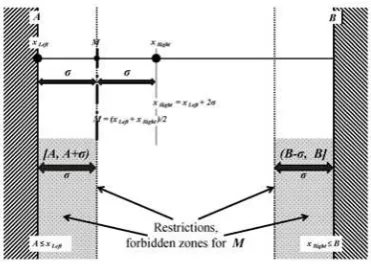
Let us assume (see, e.g., Harin, 2012a) an interval [A, B] (see Figure 1). Let us assume that two points are determined on this interval: a left point xLeft and a

right point xRight : xLeft<xRight. The coordinates of the middle mean point may be

calculated as M=(xLeft+xRight)/2.

Figure 1. An interval [A, B]. Left xLeft, right xRight and mean M points

Let us assume that xRight-xLeft≥2σ=2Constσ>0. So, of course, xRight≥xLeft+2σ

and xLeft≤xRight-2σ. For the sake of simplicity, Figures 1 to 3 represent the case of

the equality xRight-xLeft=2σ and also, of course, xRight=xLeft+2σ, xLeft=xRight-2σ and M-xLeft=xRight-M=σ=Constσ>0.

So, M=xLeft+σ>xLeft and M=xRight-σ<xRight.

Suppose further that xLeft≥A and xRight≤B.

One can easily see that two types of zones for M can exist in the interval: (1) The mean point M can be located only in the zone which will be referred to as "allowed" (see Figure 2).

(2) The mean point M cannot be located in the zones which will be referred to as "forbidden" (see Figure 3).

Allowed zone

19

The sample conditions mean that the left point xLeft may not be located

further left than the left border of the interval xLeft≥A and the right point xRight may

not be located further right than the right border of the interval xRight≤B.

For M, we have M=xLeft+σ≥A+σ>A and M=xRight-σ≤B-σ<B (see Figure 2).

The width of the allowed zone for M is equal to

σ

σ

σ

− A B A

B

It is less than the width (B-A) of the total interval [A, B] by 2σ. Also, the

allowed zone is a proper subset of the total interval.

If the distance 2σ between the left xLeft and right xRight points is non-zero,

then the difference between the width of the allowed zone and the width of the interval is non-zero also. If the distance is greater than 2σ, then the difference is greater than 2σ also.

So, the mean point M can be located only in the allowed zone of the interval.

Forbidden zones, restrictions

The value of a restriction or the width of a forbidden zone signifies the minimal possible distance between the mean and a border of the interval. For the sake of brevity, the term "the value of a restriction" may be shortened to "restriction."

If A≤xLeft, xRight≤B and xRight-xLeft=2σ, then restrictions, forbidden zones

with the width of one sigma σ , exist between the mean point and the borders of the interval (see Figure 3). So there are two forbidden zones, located near the borders of the interval. The mean point M cannot be located in these forbidden zones.

Figure 3. Forbidden zones, restrictions on M

The restrictions, the forbidden zones, are shown by two dotted lines and by painting in the bottom part of Figure 3.

As we can easily see, restrictions on the mean or forbidden zones exist between the allowed zone of the mean M and the borders A and B of the interval

[A; B]. The value of the restriction, or, equivalently, the width of the forbidden zone, is equal to σ.

20

Restrictions on the probability

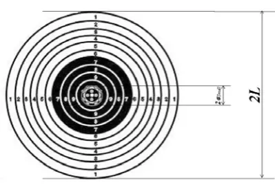
Let us consider (see, e.g., Harin, 2012a) a classical example: firing at a target. Suppose a round target (Figure 4) of diameter 2L.

Figure 4. Firing target

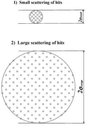
Let us suppose (Figure 5) the dispersion of hits is uniformly (for the obviousness) distributed in a zone of diameter 2σ (see an example of the normal

distribution, e.g., in Harin 2010a). Let us consider two cases:

(1) The diameter 2σSmall of the zone of dispersion of hits is considerably

smaller than the diameter 2L of the target (small dispersion).

(2) The diameter 2σLarge of the zone of dispersion of hits is considerably

larger than the diameter 2L of the target (large dispersion).

21 Notes on the figure:

Note 1: This is only a simplified example (see an example of the normal distribution, e.g., in Harin 2010a).

Note 2: Case 1 represents a small diameter 2σSmall of the zone of dispersion of

hits.

Case 2 represents a large diameter 2σLarge of the zone of dispersion of hits.

Suppose the aiming point varies between the center of the target and a point which is outside the target.

Small dispersion

Figure 6. Small dispersion of hits

Small dispersion occurs when the diameter 2σSmall of the zone of dispersion of

hits is considerably smaller than the diameter 2L of the target, as drawn in Figure 6. Notes:

The diameter 2σSmall of the zone of dispersion of hits is considerably smaller

than the diameter 2L of the target.

In the condition of the small dispersion of hits, the maximum possible probability of hitting the target can be equal to one (can reach the boundary of the probability scale).

When the point of aim varies between the center of the target and a point which is outside the target, the probability of hitting the target ranges from one to

22

Large dispersion. Restrictions

The case when the diameter 2σLarge of the zone of dispersion of hits is

considerably larger than the diameter 2L of the target is drawn in Figure 7.

Figure 7. Large dispersion of hits

Note: The diameter 2σLarge of the zone of dispersion of hits is considerably

larger than the diameter 2L of the target.

At the condition of the large dispersion of hits (that is, when the diameter

2σLarge of the zone of dispersion of hits is larger than the diameter 2L of a target),

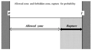
the maximum possible probability of hitting the target cannot be equal to one. The probability for this case is shown in Figure 8.

Figure 8. Restriction for the probability: Allowed zone and forbidden zone

The value PAllowedMax of the maximal allowed probability of the allowed zone

[0, PAllowedMax] may be estimated as the ratio of the mean number of the hits on the

23

4.2.2. Applications of the hypothesis 4.2.2.1. Partial explanation of Ellsberg paradox

Experiment

Let us briefly review the application of the hypothesis to the Ellsberg paradox (in more detail see, e.g., Harin, 2008a).

The Ellsberg paradox (see Ellsberg, 1961) ( here simplified and modified): the urn U1 (certain) contains red and black balls with certain proportion 1:1. the urn U2 (uncertain) contains red and black balls with unknown proportion. You will win $100 if you draw a ball of the determined color from the urns U1 or U2. Most people state that they prefer the certain U1 to the uncertain U2 for both red and black balls.

The situation can be described as

1

_ _

Red Uncertain+PBlack Uncertain <

P ,

or, more precisely,

Certain Black Certain

d Uncertain Black Uncertain

d P P P

P_{Re _} + _{_} < _{Re _} + _{_} ,

where

PRed Certain - the probability of drawing a red ball from the certain urn U1; PBlack Certain - the probability of drawing a black ball from the certain

urn U1;

PRed Uncertain - the probability of drawing a red ball from the uncertain

urn U2;

PBlack Uncertain - the probability of drawing a black ball from the

uncertain urn U2.

Ideal, real and seeming cases

Let us suppose two types of cases:

(1) An ideal case (or an ideal point of view):

Unforeseen events cannot occur. The present probability system of a future event is complete. The total probability of the present probability system of a future event equals one (or, equivalently, 100%)

% 100

_ _

Pr =

∑

and

% 100 _

_ Re

_ _

Re

= +

=

= +

Certain Black Certain

d

Uncertain Black Uncertain

d

P P

P P

,

where

∑PPresent_for_Future - the present sum of the probabilities of posterior future

events.

24 (2) Real and seeming cases:

Unforeseen events can occur. At least one future unforeseen event can occur: this will lessen the total probability of the present probability system of a posterior future event. The total probability of the present probability system of a future event is less than 100%. Indeed, if

∑

∑

= PPresent_for_Future PUnforeseen

%

100

and

0

>

∑

then

% 100

_ _

Pr <

∑

and

% 100

_ _

Red Uncertain+PBlack Uncertain <

P

and

% 100

_ _

Red Certain+PBlack Certain <

P ,

where

∑PUnforeseen - the sum of the probabilities of unforeseen events.

Let us suppose a supplementary assumption: Suppose there are two present situations: a certain present situation and an uncertain one.

Let us assume that the sum of the probabilities of unforeseen events for the certain present situation is less than that for the uncertain present situation.

Because of this assumption, the total probability of the present probability system of a future event for the certain present situation is more than the total probability of the present probability system of the future event for the uncertain present situation. So a difference between the sum of the probabilities of unforeseen events for the uncertain and certain present situation can exist.

Human experience can reveal the existence of the non-zero sum of the probabilities of unforeseen events. So, humans can feel that there is the zero sum of the probabilities of unforeseen events. The whole of the preceding experience can lead to an averaged perceptible sum of the probabilities of unforeseen events. The sum of the probabilities of unforeseen events for a particular situation can differ from the averaged sum. So, one may bear in mind that there is the seeming sum of the probabilities of unforeseen events. The difference between the sum of the probabilities of unforeseen events for the uncertain and certain present situation can be both real and seeming. So, one may bear in mind either the real or seeming difference between the sum of the probabilities of unforeseen events for the uncertain and certain present situation.

25

Transformation and bias

Suppose a transformation from an ideal to a real case. This corresponds to the transformation from the ideal point of view to the point of view of the people.

The ideal probability PIdeal is transformed to some real or seeming probability PReal.

Because of the above assumption, the real or seeming difference between the sum of the probabilities of unforeseen events for the uncertain and certain present situation is increased from the ideal case of zero to the real case of some non-zero magnitude, say to δPReal-Ideal=0.000001%>0.

Therefore, for two types of cases we obtain:

In the ideal case (or from the ideal point of view), the difference between the sum of the probabilities of unforeseen events for the uncertain and certain present situation equals zero.

In the real case (or from the point of view of the people), the real or seeming difference between the sum of the probabilities of unforeseen events for the uncertain and certain present situation equals zero.

So, there is the non-zero bias of probability δPReal-Ideal>0 between the real (or

seeming) and ideal cases.

Because of the above bias, we obtain

Ideal al Certain

Black Certain

d

Uncertain Black

Uncertain d

P P

P

P P

−

+ +

=

= +

Re _

_ Re

_ _

Re

δ .

So, at

0

Real−Ideal >

P

δ .

we obtain

Certain Black Certain

d Uncertain Black Uncertain

d P P P

PRe _ + _ < Re _ + _ .

So, from the point of view of the first consequence of the hypothesis of uncertain future, the Ellsberg paradox is quite natural.

26

4.2.2.2. Probability weighting problems Ideal, real and seeming cases

Let us briefly review the applications of the hypothesis to probability weighting problems (in more detail see, e.g., Harin, 2012b).

Let us suppose (see, e.g., ) two types of cases:

(1) An ideal case: There is no (or negligible) dispersion of data. Hence, the probability may be equal to any value near any boundary of the probability scale. Assume a value PIdeal=100%-δ: 0<δ<<100% of the probability located near 100%

in an ideal case with zero dispersion of data.

(2) Real and seeming cases: There is a zero dispersion of data. The non-zero dispersion of the data causes a non-non-zero restriction, say rRestriction≥3%, near any

boundary of the probability scale.

The previous experience of people can lead to an averaged perceptible dispersion of data and to averaged restriction. This averaged restriction may differ from the real restriction for a particular situation. So, people may keep in mind the seeming dispersion and restriction.

From the ideal point of view, we may keep in mind no (or negligible) dispersion of data and we may propose probabilities that are very close to the boundary of the probability scale. If the real experience of people proves that the dispersion is usually large, then, contrary to the ideal point of view, they may keep in mind the real case of the large dispersion, namely of the dispersion that causes a non-zero restriction, say rRestriction≥3%.

Transformation

Suppose a transformation from an ideal to a real case. This corresponds to the transformation from the ideal point of view to the point of view of people.

The absence or negligible dispersion of data is transformed to non-zero dispersion of data. Zero value of the probability of the ideal case PIdeal will be

transformed to non-zero value of the real case PReal.

Let a restriction in the probability scale be increased from the ideal case of

zero to the real case of some non-zero magnitude, say to rRestriction=3%. The

27

Bias of probability

Consider the probability near the right boundary, 100% of the probability

scale [0%; 100%]. The probability cannot be located in the restriction. Hence, the probability PReal cannot be more than PReal≤100%-rRestriction=100%-3%=97%. If the

dispersion of data is increased to the extent that the restriction exceeds the difference between 100% and PIdeal, that is, rRestriction>δ, then PReal cannot be equal

to (or more than) PIdeal. The ideal case probability of, say, 98% cannot be located in

the restriction and is biased to a position that is not more than 97%. Every ideal probability from 97.000...01% to 99.999...99% is also biased to a corresponding real position that is not more than 97%.

So, near 100%, PReal is biased downward to the middle of the probability scale

with respect to PIdeal, that is, near 100%, PReal<PIdeal. The closer the probability PIdeal is to 100%, the greater is the bias PIdeal-PReal. Conversely, for any non-zero

restriction rRestriction>0, a PIdeal=100%-δ : δ>0 will exist, such as rRestriction>δ>0, and,

hence, PReal<PIdeal.

An analogous consideration may be performed for a probability located near

0% (keeping in mind the first consequence of the hypothesis).

So, the restrictions near the boundaries shift and bias the probability from the boundaries to the middle of the probability scale. The bias is directed to the middle and is maximal just near every boundary.

Therefore, in the ideal case (or from the ideal point of view), the probability is unbiased. In the real case (or from the point of view of people), the probability near every boundary is biased (in comparison with the ideal case) from the boundary to the middle of the probability scale. Taking into account the restrictions and the biases may help to overcome the influence of observation noise, and to refine the results of experiments.

Note that the bias may be assumed to exist not only in the zones of the restrictions but also beyond them and to vanish at the middle of the scale.

28

Underweighting of high probabilities Gain at high probabilities. Deposits

Let us assume that we offer a choice of two outcomes:

(A) a guaranteed gain of a prize of $99 (with the probability 1 or 100%) or

(B) a probable gain of $100 with the probability 0.99 (or 99%), or nothing with the probability 0.01 (or 1%).

For experimental accuracy, both $99 and $100 should be in $1 banknotes, i.e.

99 and 100 banknotes of $1.

A real example: Despite the publicity and obvious advantages of bank deposits, people are not willing to use them as often and as much as predicted by the probability theory.

In the ideal case and from the ideal point of view, the probable gain has the probability 99% and the mean values for the probable and guaranteed outcomes are

99 $ % 100 99

$ × =

and

99 $ % 99 100

$ × = .

Here

99 $ % 99 100

$ × = .

The mean value of obtaining the probable gain is evidently precisely equal to the mean value of obtaining the guaranteed gain.

The well-determined experimental fact, however, is this: in similar experiments for gains at high probabilities the overwhelming majority of people choose the guaranteed gain instead of the probable one (see, e.g., Tversky and Wakker, 1995, Di Mauro and Maffioletti, 2004). People underestimate probable outcomes and do not like risk.

In the real case and from the point of view of people, if the dispersion of real data leads to the restriction (near 100%) that is more than 1% and is equal to, say,

3%, then the probability of the probable gain cannot be equal to 99% and is not more than 97%

99 $ % 100 99

$ × =

and

97 $ % 97 100

$ × = .

Here

97 $ % 97 100

$ × = .

The mean value of the probable gain is less than the mean value of the guaranteed gain.

So, in the real case and from the point of view of people, the mean of the probable gain is less than the mean of the guaranteed gain and the guaranteed outcome is preferable.

29

Overweighting of low probabilities Gain at low probabilities. Lotteries

Let us assume that we offer a choice of two outcomes: (A) a guaranteed gain of $1 (with the probability 100%) or

(B) a probable gain of a prize of $100 with the probability 0.01 (or 1%), or nothing with the probability 0.99 (or 99%).

A real example: Obviously the organizers of lotteries are paid from the lottery proceeds and people usually do not gain as much from lotteries as they pay in. Nevertheless, they are very willing to participate all the same.

In the ideal case and from the ideal point of view, the probable gain has the probability 1% and the mean values for the probable and guaranteed outcomes are

1 $ % 100 1

$ × = and

1 $ % 1 100

$ × = . Here

1 $ 1

$ = .

The mean value for obtaining the probable gain is precisely equal to the mean value for obtaining the guaranteed gain.

The well-determined experimental fact is this, however: in similar experiments on gains at low probabilities the overwhelming majority of people choose the probable gain instead of the guaranteed one (see, e.g., Tversky and Wakker, 1995, Di Mauro and Maffioletti, 2004). People overestimate probable outcomes and do not like risk.

In the real or seeming cases and from the point of view of people, if the dispersion of real data leads to the restriction (near 0%) that is more than 1% and is equal to, say, 3%, then the probability of the probable gain may be (keeping in mind the decreasing probability because of the first consequence of the hypothesis) 3% or more

1 $ % 100 1

$ × = and

3 $ % 3 100

$ × = . Here

1 $ 3

$ > .

The mean value of the guaranteed gain may be less than the mean value of the probable gain.

So, in the real or seeming cases and from the point of view of people, the mean of the guaranteed gain may be less than the mean of the probable gain and the probable outcome is preferable.

30 Gains and losses

Loss at high probabilities. Defaults

Let us assume that we offer a choice of two outcomes:

(A) a guaranteed loss of -$99 (with the probability 1 (or 100%)) or

(B) a probable loss of -$100 with the probability 0.99 (or 99%), or no loss with the probability 0.01 (or 1%).

A real example: It is clear that the earlier one declares a default, the less one will lose. Nevertheless, often people and even governments delay declaring a default.

In the ideal case and from the ideal point of view, the probable loss has the probability 0.99 (or 99%) and the mean values for the probable and guaranteed outcomes are

99 $ % 100 99

$ × =−

−

and

99 $ % 99 100

$ × =−

− .

Here

99 $ 99 $ =−

− .

The mean value of the probable loss is precisely equal to the mean value of the guaranteed loss.

The well-determined experimental fact, however, is this: in similar experiments for gains at high probabilities the overwhelming majority of people choose the probable loss instead of the guaranteed one (see, e.g., Tversky and Wakker, 1995, Di Mauro and Maffioletti, 2004). People overestimate probable outcomes and like risk.

In the real case and from the point of view of people, if the dispersion of real data leads to the restriction (near 100%) that is more than 1% and is equal to, say,

3%, then the probability of the probable loss cannot be equal to 99% and is not more than 97%

99 $ % 100 99

$ × =−

−

and

97 $ % 97 100

$ × =−

− .

Here

97 $ 99 $ <− − .

The mean value of the probable gain is less than the mean value of the guaranteed gain.

So, in the real case and from the point of view of people, the mean of the guaranteed loss is less than the mean of the probable loss (it is less in terms of absolute value but more because of the negative sign of the loss). Hence, the probable outcome is preferable.

31

Conclusions

So, the unforeseen events can essentially modify forecasts and increase financial risks. But their negative influence can be lessened by the preliminary risk management in some cases of the partially unforeseen events. For example, if the influence of a partially unforeseen event could be and was preliminary (partially) estimated, then this estimate may be used just after this event has occurred.

At present, it is evident, that a forecast should manifestly contain errors’ terms. A long-term forecast should manifestly contain unforeseen errors’ terms (because the relative error, caused by an unforeseen event, can be much more than 100%). A long-use forecast should contain correcting terms. These terms may have the form of a framework for forecasts – a correcting formula for forecasts.

This correcting formula for forecasts may be used as a correcting tool for long-use forecasts and as an adapting tool in addition to unified forecasts to apply them to special situations.

Let us suppose that the modification ΔF(tBase, tCorr, t) of the forecast function

may be exactly or approximately expressed in the form of explicit functions. The operations of addition and multiplication are, probably, the most common and important ones as in practice so in the pure mathematics (see, e.g., Waerden van der, 1976). If we suppose that the ΔF(tBase, tCorr, t) may be exactly or approximately

expressed by means of additive and multiplicative functions, then the formula

] 1 [ ] ) , ( ) , ( ) , ( [ ) , , ( 1 , 1 , Error A a Corr a Addit M m Corr m t Multiplica Base Base Corr Base t t t t K t t F t t t F ∆ ± × Φ + × ≈

∑

∏

may be written, or, omitting the variables and indices, it may be written in the form

] 1

[ ]

[FBase KMultiplicat Addit Error

F ≈ ×

∏

∑

For the cases when

0 ) , ( ) , ( 1 , ≠ ×

∏

Base t t K t t

F ,

(preferentially for F~Fbase) this formula may be written as

] 1 [ )] , ( 1 [ ] )) , ( 1 ( [ ) , ( ) , , ( 1 , 1 , Error A a Corr a Addit M m Corr i t Multiplica Base Base Corr Base t t t t k t t F t t t F ∆ ± × + × + × ≈

∑

∏

or, omitting the variables and indices,

] 1 [ ] 1 [ )] 1 (

[ _{Multiplicat Addit Error}

Base k

F

F ≈ ×

∏

∑

We may easily obtain the transformations between the versions of the formula.

For multiplicative functions

m t Multiplica m t Multiplica k

K , =1+ , .

For additive functions

∏

Addit F k

1

, ,

32

References

Caporin, M.; McAleer, M., 2011. “Thresholds, news impact surfaces and dynamic asymmetric multivariate GARCH”, Statistica Neerlandica, Vol. 65, 125-163. Caporin, M.; McAleer, M., 2010. “A scientific classification of volatility models”,

Journal of Economic Surveys, Vol. 24, pp. 192-195.

Castle, J.; Doornik, J.; Hendry, D., 2012. “Model selection when there are multiple breaks”, Journal of Econometrics, Vol. 169(2), pp. 239-246.

Chang, C.; Franses, P.; McAleer, M., 2011. “How accurate are government forecasts of economic fundamentals? The case of Taiwan”, International Journal of Forecasting, Vol. 27, pp. 1066-1075.

Clements, M.; Hendry, D., 2006. “Forecasting with Breaks”, in: Elliott, G., Granger, C. and Timmermann, A. (Eds.), Handbook of Economic Forecasting. Elsevier; Volume 1, pp. 605-657.

Ellsberg, L., 1961, “Risk, Ambiguity, and the Savage Axioms”, The Quarterly Journal of Economics, Vol. 75 (4), pp. 643-669.

Di Mauro, C. and Maffioletti, A. 2004. “Attitudes to risk and attitudes to uncertainty: experimental evidence”, Applied Economics, Vol. 36, pp. 357-372.

Heisenberg, W., 1927. “Über den anschaulichen Inhalt der quantentheoretischen Kinematik und Mechanik”, Zeitschrift für Physik. Vol. 43: 172-198.

Hendry, D.F.; Mizon, G.E., 2013. “Unpredictability in Economic Analysis, Econometric Modeling and Forecasting”, Economics Series Working Papers from University of Oxford, Department of Economics, 2013-W04.

Harin, A., 2004. “Arrangement infringement possibility approach: some economic features of large-scale events”, Research Announcements, Economics Bulletin, Vol. 28, issue 11, pages A0.

Harin, A., 2005. “A Rational Irrational Man”, Public Economics from Economics Working Paper Archive at WUSTL, 0511005.

Harin, A., 2007a. “Principle of uncertain future, examples of its application in economics, potentials of its applications in theories of complex systems, in set theory, probability theory and logic”, Proceedings of the Seventh International Scientific School "Modeling and Analysis of Safety and Risk in Complex Systems", Saint Petersburg, Russia, September 4-8.

Harin, A., 2007b. “Principle of uncertain future and utility”, MPRA Paper from University Library of Munich, Germany, 1959.

Harin, A., 2008a. “Solution of the Ellsberg paradox by means of the principle of uncertain future”, MPRA Paper from University Library of Munich, Germany, 8168.

33

Harin, A., 2009a. “General correcting formula of forecasting?”, MPRA Paper from University Library of Munich, Germany, 15746.

Harin, A., 2009b. “Ruptures in the probability scale? Calculation of ruptures’ dimensions”, MPRA Paper from University Library of Munich, Germany, 19348.

Harin А. 2010a. “Theorem of existence of ruptures in the probability scale”, 9th International conference "Financial and Actuarial Mathematics and Eventoconverging Technologies", Krasnoyarsk.

Harin А., 2010b. “РАЗРЫВЫ В ШКАЛЕ ВЕРОЯТНОСТЕЙ. ИХ

ПРОЯВЛЕНИЯ В ЭКОНОМИКЕ И ПРОГНОЗИРОВАНИИ”, EconStor Open Access Articles, 10419/60194.

Harin А., 2011. “ТЕОРЕМЫ О СУЩЕСТВОВАНИИ РАЗРЫВОВ НА

ЧИСЛОВЫХ ОТРЕЗКАХ И В ШКАЛЕ ВЕРОЯТНОСТЕЙ И НЕКОТОРЫЕ ВОЗМОЖНОСТИ ИХ ПРИМЕНЕНИЯ”, EconStor Open Access Articles, 10419/58193.

Harin А. 2012a. “Data Dispersion in Economics (I) --- Possibility of Restrictions”, Review of Economics & Finance, Vol. 2(3), pp. 59-70.

Harin А., 2012b. “Data Dispersion in Economics(II)--- Inevitability and Consequences of Restrictions”, Review of Economics & Finance, Vol. 2(4), pp. 24-36.

Harin, A., 2013. “Data dispersion near the boundaries: can it partially explain the problems of decision and utility theories?”, Working Papers from HAL, 00851022.

McAleer, M.; Medeiros, M.; Slottje, D., 2008. “A neural network demand system with heteroskedastic errors”. Journal of Econometrics, Vol. 147, pp. 359-371. Morlidge, S., 2013. “How good is a "good" forecast?: Forecast errors and their

avoidability”. Foresight: The International Journal of Applied Forecasting, Vol. 30, pp. 5-11.

Tversky, A., and Wakker, P., 1995. “Risk attitudes and decision weights”, Econometrica, Vol. 63, pp. 1255-1280.