A dissertation submitted to the University of Dublin for the degree of Doctor of Philosophy
Andrew Hines
Trinity College Dublin, January 2012
For Alan
Hearing impairment, and specifically sensorineural hearing loss, is an increasingly prevalent condition, especially amongst the ageing population. It occurs primarily as a result of damage to hair cells that act as sound receptors in the inner ear and causes a variety of hearing percep-tion problems, most notably a reducpercep-tion in speech intelligibility. Accurate diagnosis of hearing impairments is a time consuming process and is complicated by the reliance on indirect measure-ments based on patient feedback due to the inaccessible nature of the inner ear. The challenges of designing hearing aids to counteract sensorineural hearing losses are further compounded by the wide range of severities and symptoms experienced by hearing impaired listeners.
Computer models of the auditory periphery have been developed, based on phenomenological measurements from auditory-nerve fibres using a range of test sounds and varied conditions. It has been demonstrated that auditory-nerve representations of vowels in normal and noise-damaged ears can be ranked by a subjective visual inspection of how the impaired representations differ from the normal. This thesis seeks to expand on this procedure to use full word tests rather than single vowels, and to replace manual inspection with an automated approach using a quantitative measure. It presents a measure that can predict speech intelligibility in a consistent and reproducible manner. This new approach has practical applications as it could allow speech-processing algorithms for hearing aids to be objectively tested in early stage development without having to resort to extensive human trials.
Simulated hearing tests were carried out by substituting real listeners with the auditory model. A range of signal processing techniques were used to measure the model’s auditory-nerve outputs by presenting them spectro-temporally as neurograms. A neurogram similarity index measure (NSIM) was developed that allowed the impaired outputs to be compared to a reference output from a normal hearing listener simulation. A simulated listener test was developed, using standard listener test material, and was validated for predicting normal hearing speech intelligibility in quiet and noisy conditions. Two types of neurograms were assessed: temporal fine structure (TFS) which retained spike timing information; and average discharge rate or temporal envelope (ENV). Tests were carried out to simulate a wide range of sensorineural hearing losses and the results were compared to real listeners’ unaided and aided performance. Simulations to predict speech intelligibility performance of NAL-RP and DSL 4.0 hearing aid fitting algorithms were undertaken. The NAL-RP hearing aid fitting algorithm was adapted using a chimaera sound algorithm which aimed to improve the TFS speech cues available to aided hearing impaired listeners.
I hereby declare that this thesis has not been submitted as an exercise for a degree at this or any other University and that it is entirely my own work.
I agree that the Library may lend or copy this thesis upon request.
Signed,
Andrew Hines
Contents vii
List of Figures xi
List of Acronyms and Abbreviations xiii
1 Introduction 1
1.1 Thesis outline . . . 1
1.2 Contributions of this thesis . . . 4
1.3 Publications . . . 5
1.3.1 Journal . . . 5
1.3.2 Conference Papers . . . 5
1.3.3 Other Conference Posters and Presentations . . . 6
2 Background 7 2.1 Peripheral Auditory Anatomy and Physiology . . . 7
2.1.1 Outer and Middle Ears . . . 8
2.1.2 Inner Ear . . . 9
2.1.3 Tuning on the Basilar Membrane . . . 10
2.1.4 Auditory Nerve Characteristics . . . 10
2.1.5 Beyond the Auditory Periphery . . . 11
2.2 Sensorineural Hearing Loss . . . 12
2.2.1 Thresholds and Audiograms . . . 14
2.3 Auditory Periphery Model . . . 14
2.3.1 Phenomenological Models . . . 15
2.3.2 Perceptual Models . . . 17
2.4 Neurograms . . . 18
2.4.1 Speech Signal Analysis . . . 18
2.4.2 Neurogram representations of speech . . . 20
2.5 Speech Perception and Intelligibility . . . 26
2.5.1 Speech Perception . . . 26
2.5.2 Quantifying Audibility . . . 27
2.5.3 Speech Intelligibility and Speech Quality . . . 28
2.5.4 Speech Intelligibility Index and Articulation Index . . . 29
2.5.5 Speech Transmission Index . . . 30
2.5.6 Speech Intelligibility for Hearing Impaired Listeners . . . 30
2.5.7 Spectro-Temporal Modulation Index (STMI) . . . 30
2.5.8 Neural Articulation Index (NAI) . . . 31
2.6 Image Similarity Metrics for Neurogram Comparisons . . . 32
2.6.1 Mean Squared Error and Mean Absolute Error . . . 33
2.6.2 Structural Similarity Index (SSIM) . . . 34
2.6.3 Structural Similarity Index for Neurograms . . . 37
2.6.4 Neurogram SSIM for Speech Intelligibility . . . 39
2.7 Hearing Aid Algorithms . . . 40
2.7.1 History of Hearing Aids . . . 40
2.7.2 Prescribing Hearing Aid Gains . . . 40
2.7.3 NAL . . . 41
2.7.4 DSL . . . 42
2.7.5 Non-linear Fitting Methods . . . 42
2.7.6 Hearing Aid Comparisons and the Contributions of this Thesis . . . 42
3 Speech Intelligibility from Image Processing 45 3.1 Introduction . . . 45
3.2 Background . . . 46
3.2.1 Tuning the Structural Similarity Index (SSIM) . . . 46
3.3 Method . . . 49
3.3.1 Test Corpus . . . 49
3.3.2 Audiograms and Presentation Levels . . . 50
3.4 Results & Discussion . . . 53
3.4.1 SSIM Window Size . . . 53
3.4.2 SSIM Weighting . . . 54
3.4.3 Comparison of SSIM to RMAE/RMSE . . . 55
3.4.4 Effect of Hearing Loss on Neurograms . . . 55
3.4.5 Comparison to NAI . . . 56
3.4.6 Limitations of SSIM . . . 56
3.4.7 Towards a single AN fidelity metric . . . 56
3.5 Conclusions . . . 59
4.2.1 Auditory Nerve Models . . . 63
4.2.2 Neurograms . . . 63
4.2.3 Structural Similarity Index (SSIM) . . . 63
4.2.4 The Performance Intensity Function . . . 64
4.3 Simulation Method . . . 65
4.3.1 Experimental Setup . . . 66
4.4 Experiments and Results . . . 67
4.4.1 Image Similarity Metrics . . . 67
4.4.2 Neurogram Similarity Index Measure (NSIM) . . . 69
4.4.3 Accuracy and Repeatability . . . 70
4.4.4 Method and Model Validation . . . 70
4.4.5 Simulated Performance Intensity Functions (SPIFs) . . . 72
4.4.6 Comparison to SII . . . 73
4.5 Discussion . . . 74
4.5.1 Comparison with other models . . . 78
4.6 Conclusions . . . 80
5 Comparing Hearing Aid Algorithms Using Simulated Performance Intensity Functions 81 5.1 Introduction . . . 81
5.2 Background . . . 82
5.2.1 Performance Intensity Function . . . 82
5.2.2 Simulated Performance Intensity Function . . . 83
5.2.3 Hearing Profiles and Hearing Aid Algorithms . . . 83
5.3 Simulated Tests . . . 83
5.4 Hearing Losses Tested . . . 85
5.4.1 A Flat Moderate Sensorineural Hearing Loss . . . 85
5.4.2 A Flat Severe Sensorineural Loss . . . 86
5.4.3 A Severe High-Frequency Sensorineural Hearing Loss . . . 88
5.4.4 A Gently Sloping Mild Sensorineural Hearing Loss . . . 89
5.5 Discussion . . . 90
5.5.1 Simulation and Clinical Test Comparison . . . 90
5.5.2 Fitting algorithm comparisons . . . 91
5.6 Conclusions . . . 92
6 Hearing Aids and Temporal Fine Structure 93 6.1 Introduction . . . 93
6.2.1 Temporal fine structure . . . 94
6.2.2 Hearing Aids and TFS . . . 94
6.2.3 Auditory Chimaeras . . . 95
6.3 Experiment I: TFS Neurogram Similarity for Hearing Impaired Listeners . . . 96
6.3.1 Method . . . 96
6.3.2 Results and Discussion . . . 96
6.4 Experiment II: Chimaera Hearing Aids . . . 100
6.4.1 Method . . . 100
6.4.2 Results and Discussion . . . 101
6.5 General Discussion . . . 104
6.6 Conclusions . . . 105
7 Conclusion 107 7.1 Central Themes . . . 107
7.2 Applications . . . 108
7.3 Future Work . . . 108
7.3.1 Neurogram Similarity Index Measure . . . 109
7.3.2 Auditory Nerve Models . . . 109
7.3.3 Temporal Fine Structure . . . 109
7.3.4 Hearing Aid Design . . . 110
A Full Result Set for Chapter 3 113
B CASPA Word lists 117
2.1 The Peripheral Auditory System . . . 8
2.2 Anatomy of the Cochlea . . . 9
2.3 Post Stimulus Time Histogram (PSTH) . . . 11
2.4 Frequency Resolution and SNHL . . . 13
2.5 Sample audiogram showing hearing thresholds for a subject with a moderate sensorineural hearing loss. . . 15
2.6 Schematic diagram of the Zilany et al. [102] AN model . . . 17
2.7 Sample Signal Envelope and Temporal Fine Structure . . . 19
2.8 Sample Signal Envelope and Temporal Fine Structure (close up) . . . 20
2.9 Sample Neurograms . . . 21
2.10 Sample PSTHs, 10µs and 100µs bins . . . 23
2.11 Sample TFS Neurogram . . . 24
2.12 Sample ENV Neurogram . . . 25
2.13 Neurogram examples of phonemes from the 6 TIMIT phoneme groupings . . . . 26
2.14 Spectrograms for the sounds /ba/ and /da/ . . . 27
2.15 Block diagram: from speaker to listener . . . 28
2.16 Sample Neurograms at 65, 30 and 15 dB SPL . . . 33
2.17 SSIM Image Comparisons: Einstein . . . 35
2.18 SSIM Neurogram Comparisons . . . 36
2.19 REAG, REUG, REIG relationship . . . 41
3.1 Sample ENV and TFS neurograms for fricative /sh/ with progressively degrading hearing loss . . . 47
3.2 Sample ENV and TFS neurograms for a vowel (/aa/) with progressively degrading hearing loss . . . 48
3.3 Block diagram of Chapter 3 method . . . 49
3.4 Audiograms of hearing losses tested . . . 50
3.5 Illustrative view of window sizes reported on a TFS vowel neurogram . . . 51
3.6 SSIM Results varying metric’s window size and component weightings . . . 52
3.7 Comparison of results for RMAE, RMSE and SSIM . . . 53
3.8 Spider plot 65 dB SPL results for all phoneme groups using RMAE, RMSE and
SSIM . . . 57
3.9 Spider plot 85 dB SPL results for all phoneme groups using RMAE, RMSE and SSIM . . . 58
3.10 SII for hearing losses . . . 59
3.11 Comparison of results to SII . . . 60
4.1 The Simulated Performance Intensity Function . . . 62
4.2 Block diagram of Chapter 4 method . . . 65
4.3 PI functions simulated using AN model data from ten word lists comparing image similarity metrics . . . 68
4.4 Optimal component weightings for SSIM . . . 69
4.5 AN model variance test results . . . 71
4.6 Word list test results . . . 72
4.7 SSIM results for 10 lists . . . 73
4.8 Spectrogram results . . . 74
4.9 Simulated performance intensity functions in quiet . . . 75
4.10 Simulated performance intensity functions in noise . . . 76
5.1 Block diagram of Chapter 5 method . . . 84
5.2 Audiogram and Results: a flat moderate hearing loss . . . 86
5.3 Audiogram and Results: a flat severe hearing loss . . . 87
5.4 Audiogram and Results: a high-frequency severe hearing loss . . . 88
5.5 Audiogram and Results: a mild gently sloping hearing loss . . . 89
5.6 Real listener test results for a flat moderate sensorineural hearing loss . . . 90
6.1 Aided chimaera synthesis . . . 95
6.2 ENV NSIM results, unaided and aided . . . 97
6.3 TFS NSIM results, unaided and aided . . . 98
6.4 Vowel NSIM results . . . 99
6.5 Block diagram of Chapter 6, exp. II method . . . 100
6.6 Chimaera aid results . . . 101
6.7 RMS presentation levels for aided words . . . 102
6.8 Sample neurograms of vowel /ow/: unaided, aided and chimaera aided . . . 103
A.1 Affricate and Nasal results from Chapter 3 . . . 114
AN Auditory Nerve
ANSI American National Standards Institute
AI Articulation Index
BF Best Frequency
CASPA Computer-aided speech perception assessment
CF Characteristic Frequency
CVC Consonant-Vowel-Consonant
DSL Desired Sensation Level (hearing aid fitting method)
ENV Envelope/Average Discharge Neurogram
HASQI Hearing-Aid Speech Quality Index
HI Hearing Impaired
HL Hearing Level (dB HL)
ISM Image Similarity Metric
MCL Most Comfortable Level
MTF Modular Transfer Function
NAI Neural Articulation Index
NAL-RP National Acousitcs Laborotory, Revised Profound (hearing aid fitting method)
NH Normal Hearing
NPRT Neurogram Phoneme Recognition Threshold
NSIM Neurogram Similarity Index Measure
NU-6 Northwester University Word List # 6
PEMO-Q Perception Model - Quality
PD Phoneme Discrimination
PI Performance Intensity (function)
PRT Phoneme Recognition Threshold
PSTH Post Stimulus Time Histogram
REAG Real Ear Aided Gain
REUG Real Ear Unaided Gain
REIG Real Ear Insertion Gain
RMAE Relative Mean Absolute Error
RMSD Root Mean Square Deviation
RMSE Relative Mean Squared Error
SII Speech Intelligibility Index
SNHL Sensorineural Hearing Loss
SNR Signal to Noise Ratio
SPIF Simulated Performance Intensity Function
SPL Sound Pressure Level (dB SPL)
SRT Speech Reception Threshold
SSIM Structural Similarity Index Measure
STI Speech Transmission Index
STFT Short-Time Fourier Transform
STMI Spectro-Temporal Modulation Index
TIMIT Texas Instruments (TI) and Massachusetts Institute of Technology (MIT) Speech
Cor-pus
1
Introduction
1.1
Thesis outline
This thesis seeks to develop a novel approach to prediction of speech intelligibility using a computational model of the auditory periphery. The auditory periphery is composed of bio-mechanics that pre-filter and attenuate acoustic stimuli in the outer and middle ear before presenting the signal to frequency-tuned hair cells along the basilar membrane in the cochlea. The hair cells vibrate causing an electro-chemical potential difference that innervates an impulse firing electrostatic signal along an auditory nerve fibre. The combined firings along multiple fibres reacting to hair cells along the frequency tuned range provide a spectral slice of information on the input stimuli signal and, when evaluated temporally, these auditory nerve firings provide a spectro-temporal signal of the acoustic stimuli which is then presented to the central nervous system and brain. We call this process hearing.
The signal processing involved in the path from a speech stimuli input to an auditory nerve fibre output can be modelled using a computational model of the auditory periphery. Such a model is used here to experiment how signal processing techniques can be applied in novel ways to assess auditory nerve outputs and predict speech intelligibility for listeners under a variety of conditions and with varying degrees of hearing impairment.
The practical application of this is to allow speech-processing algorithms for hearing aids to be objectively tested in early stage development, without having to resort to extensive human trials. The proposed strategy is to harness the work that has been done in developing realistic computational models of the auditory periphery and to apply it in a process to quantitatively
predict speech intelligibility. This could be used to design hearing aids by restoring patterns of auditory nerve activity to be closer to normal, rather than focusing on human perception of sounds. Sachs et al. [72] showed that auditory-nerve discharge patterns in response to sounds as complex as speech can be accurately modelled, and predicted that this knowledge could be used to test new strategies for hearing-aid signal processing. They demonstrated examples of auditory-nerve representations of vowels in normal and noise-damaged ears and discussed, using subjective visual inspection, how the impaired representations differ from the normal. This work seeks to automate this inspection process using an objective measure that ranks hearing losses based on auditory-nerve discharge patterns. It develops a procedure to link the objective ranking measure to listener speech discrimination scores and validates the procedure in a range of conditions for a range of hearing impairments.
The remainder of this thesis is organised as follows:
Chapter 2: Background
The background provides a context for the thesis, describing the physiology of the auditory periphery and how computational models have been developed over the last four decades. Neu-rograms, a visualisation of the output from the auditory nerve model, are defined and details are presented on how they are created and assessed. Assessment methodologies for measuring speech intelligibility are reviewed along with the image similarity metrics used in this thesis to predict speech intelligibility. Hearing impairment, sensorineural hearing loss and hearing aids are also introduced.
Chapter 3: Speech Intelligibility from Image Processing
Traditionally, hearing loss research has been based on perceptual criteria, speech intelligibility and threshold levels. The development of computational models of the auditory-periphery has allowed experimentation, via simulation, to provide quantitative, repeatable results at a more granular level than would be practical with clinical research on human subjects. The responses of the auditory nerve model used in this thesis have been shown, by the model developers, to be consistent with a wide range of physiological data from both normal and impaired ears for stimuli presentation levels spanning the dynamic range of hearing.
The metric’s boundedness and the results for TFS neurograms indicate that it is a superior metric to standard point to point metrics of relative mean absolute error and relative mean squared error. SSIM as an indicative score of intelligibility is also promising, with results similar to those of the standard Speech Intelligibility Index metric.
Chapter 4: Speech Intelligibility prediction using a Neurogram Similarity In-dex Measure
Discharge patterns produced by fibres from normal and impaired auditory nerves in response to speech and other complex sounds can be discriminated subjectively through visual inspection. Similarly, responses from auditory nerves, where speech is presented at diminishing sound levels, progressively deteriorate from those at normal listening levels. This chapter presents a Neuro-gram Similarity Index Measure (NSIM) that automates this inspection process, and translates the response pattern differences into a bounded discrimination metric.
The Performance Intensity function can be used to provide additional information over mea-surement of speech reception threshold and maximum phoneme recognition, by plotting a test subject’s recognition probability over a range of sound intensities. A computational model of the auditory periphery is used to replace the human subject and develop a methodology that simulates a real listener test. The newly developed NSIM is used to evaluate the model outputs in response to Consonant-Vowel-Consonant (CVC) word lists and to produce phoneme discrim-ination scores. The simulated results are rigorously compared to those from normal hearing subjects. The accuracy of the tests and the minimum number of word lists necessary for re-peatable results are established. The experiments demonstrate that the proposed Simulated Performance Intensity Function (SPIF) produces results with confidence intervals within the human error bounds expected with real listener tests. This represents an important step in validating the use of auditory nerve models to predict speech intelligibility.
Chapter 5: Comparing hearing aid algorithm performance using Simulated Performance Intensity Functions
models to predict speech intelligibility for different hearing aid fitting methods in a simulated environment, allowing the potential for rapid prototyping and early design assessment of new hearing aid algorithms.
Chapter 6: Hearing Aids and Temporal Fine Structure
The results presented in Chapter 5 demonstrated that, for a range of hearing impairments, the Neurogram Similarity Index Measure (NSIM) could be used to simulate Performance Intensity (PI) functions that reproduced the results for human listeners when measured on ENV neuro-grams. This chapter looks at the results from the same simulated listener tests, using NSIM to measure TFS neurogram similarity. The results for unimpaired listeners, and those of listeners with gently sloping mild, flat moderate and flat severe SNHLs are compared in unaided and aided scenarios. A second experiment looks at a novel approach with an adapted hearing aid fitting algorithm and aims to improve the TFS information available for aided hearing impaired listeners. In addition, the experiment demonstrates the potential application of auditory nerve models in the development of new hearing aid algorithm designs.
Chapter 7: Conclusions
The final chapter reviews the central themes, applications and contributions of this thesis before looking at some potential directions for future work.
1.2
Contributions of this thesis
This thesis developed the Neurogram Similarity Index Measure (NSIM), a novel, image process-ing based measure to compare the similarity between auditory nerve discharge patterns. Usprocess-ing this measure and a computational model of the auditory periphery, speech intelligibility can be predicted for both normal and hearing impaired listeners. The contributions are summarised by chapter in the list below.
Chapter 3
Demonstrated that the AN model can rank progressive SNHLs
Presented the first large scale test for speech with the AN model, using a variety of speakers and a range of presentation levels
Identified the potential for the use of an image similarity measure (SSIM) rather than a basic point-to-point error metric in neurogram comparison
Chapter 4
Validated the reliability of simulating performance intensity function’s phoneme discrimi-nation predictions in normal hearing listeners and compared results with SII
Chapter 5
Validated the reliability of simulating performance intensity functions using NSIM for a range of SNHLs
Compared the predicted speech intelligibility improvements provided by two hearing aid fitting prescriptions
Chapter 6
Compared the loss of fine timing cues compared to envelope cues for a range of SNHLs
Proposed a new hearing aid fitting algorithm to optimise both envelope and fine timing cues and simulated tests to predict the speech intelligibility compared to a standard fitting algorithm
1.3
Publications
Portions of the work described in this thesis have appeared in the following publications:
1.3.1 Journal
A. Hines and N. Harte. Speech intelligibility from image processing. Speech Communica-tion, 52(9):736–752, 2010.
A. Hines and N. Harte. Reproduction of the performance/intensity function using image processing and a computational model (A). International Journal of Audiology, 50(10): 723, 2011.
A. Hines and N. Harte. Speech intelligibility prediction using a Neurogram Similarity Index Measure. Speech Communication, 54(2):306–320, 2012.
1.3.2 Conference Papers
A. Hines and N. Harte. Measurement of phonemic degradation in sensorineural hearing loss using a computational model of the auditory periphery. InIrish Signals and Systems Conference (IET), UCD, Dublin, 2009.
A. Hines and N. Harte. Evaluating sensorineural hearing loss with an auditory nerve model using a mean structural similarity measure. In European Signal Processing Conference (EUSIPCO ’10), Aalborg, Denmark, August 2010.
A. Hines and N. Harte. Comparing hearing aid algorithm performance using Simulated Performance Intensity Functions. InSpeech perception and auditory disorders, Int. Sym-posium on Audiological and Auditory Research (ISAAR), Denmark, 2011.
A. Hines and N. Harte. Simulated performance intensity functions. In Engineering in Medicine and Biology Society Conference (EMBC), EMBS (IEEE), Boston, USA, 2011.
1.3.3 Other Conference Posters and Presentations
Oral presentation atthe British Society of Audiology Conference, Manchester, UK, August 2010.
2
Background
Evolution has developed the internal ear into a biological sub-system that is miniaturised and optimised for both performance and efficiency. Modern behind-the-ear hearing aids are similar in size to the mechanics of the auditory periphery. They are powered by small batteries that need to be replaced every few days at 1.4V with power dissipation of around 5mW and up to 10kHz frequency range. The ear uses about 14 microwatts of power at 150 mV levels and a frequency span of 10 octaves. The magnitude of the gulf between the biological and electronic is massive on every metric of efficiency and accuracy.
Despite the inner ear complexity, research into the mechanisms of hearing has helped with understanding the purpose and mechanism of the peripheral auditory system. Over the last four decades, advances in modelling have allowed computational simulations to be designed that can imitate the reaction from sound stimulus in to auditory nerve firing out with remarkable accuracy. The main contributions of this thesis are focused on speech intelligibility prediction through automated analysis of model outputs. This chapter seeks to introduce the auditory periphery and a corresponding computational model at a high level, while still providing enough detail to allow an appreciation of the model’s features.
2.1
Peripheral Auditory Anatomy and Physiology
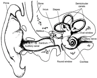
Auditory anatomy is usually divided into four distinct parts: the outer, middle and inner ear make up the auditory periphery and the final part is the central auditory nervous system (Fig. 2.1). While the central auditory nervous system and operation of the brain are critical in speech
Figure 2.1: Illustration of the structure of the peripheral auditory system showing outer, middle and inner ear. Reproduced from Moore [61], original illustration from Lindsay and Norman [49]
perception, little is known about how sound is processed into intelligible speech. According to Shamma and Micheyl [76] the number of studies that look to investigatewhereandhowauditory streams are formed in the brain has increased enormously in the last decade. Neural correlates have been found in areas traditionally unassociated with auditory processing, leading to sug-gestions that wider neural networks are involved than was previously thought. Conversely, the peripheral auditory system has been studied in detail and is well understood from an anatomical perspective. It can essentially be treated as a mechanical system and hence its operation can be modelled.
2.1.1 Outer and Middle Ears
The outer ear consists of the pinna: the visible part of the ear made of skin and cartilage; the concha or cave: the central cavity portion of the pinna; the external auditory canal: the opening leading to the eardrum; and the tympanic membrane or eardrum which is constructed of layers of tissue and fibres and is the boundary between the outer and middle ear. The primary purpose of the outer ear is to collect acoustic energy. It also provides protection, amplification and localisation functions.
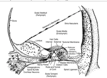
Figure 2.2: Cross-section of the cochlea, showing inner and outer hair cells and basilear mem-brane. Reproduced from Moore [61], original illustration from Davis [20]
pressure equalisation and impedance matching. It transfers the stimulus received from the outer ear via bone conduction, changes in air pressure and through the osscile bone chain.
2.1.2 Inner Ear
into around 12,000 OHCs per ear and 3500 IHCs. The hair cells are connected to auditory nerve fibres with approximately 20 fibres innervated by each IHC and 6 fibres per OHC.
2.1.3 Tuning on the Basilar Membrane
When a sound pressure wave enters the cochlea through the oval window it sets up a travelling pressure wave along the basilar membrane which is tuned along its length to different frequencies from high to low as it gets further from the stapes. At any given point, it will vibrate with its largest displacement to a best frequency known as itscharacteristic frequency (CF). Tuning curves can be measured showing the sound intensity level required to maintain a constant velocity on the basilar membrane for a range of frequencies. Such curves can measure the increase in sound pressure required to excite higher frequencies when auditory filters broaden with hearing loss.
2.1.4 Auditory Nerve Characteristics
Without acoustic stimulation, auditory neurons will fire randomly at what is termed their spon-taneous rate. According to Liberman [47], these neurons can be classified into three groups with low, medium and high minimum firing rates. These groupings are also correlated with the minimum thresholds of sound intensity to which the neuron is sensitive, with high spontaneous rate neurons having thresholds close to 0 dB SPL and low spontaneous rates having a minimum threshold of 80 dB SPL or more [61]. The dynamic range, when referring to auditory neurons, is the intensity range at which a sound pressure wave will stimulate firing. It also varies with low or medium spontaneous rate having a dynamic range between approximately 50 and 60 dB and high spontaneous rate having a smaller range between 30 and 40 dB SPL [70].
When a sinusoidal waveform stimulation is presented, nerve firings or spikes tend to occur during the positive half cycle of the stimulus period. This phenomenon is known as phase-locking [68]. While every fibre does not fire on every cycle they will fire on integer multiples of the stimulus period, meaning that a single neuron will provide definitive information about the period of the stimulus by thorough analysis of its temporal firing pattern. This can be seen by plotting a histogram of the interspike interval, as the frequency of the sinusoidal waveform stimulation will determine the histogram distribution. An interspike interval histogram allows the time interval between successive neural spikes to be measured with the time between spikes on the x-axis and the number of spikes on the y-axis.
At the onset of a stimulus, the spike discharge rate rapidly rises over the first few milliseconds. It then drops to a lower steady state for the duration of the stimulus period, which is known as
Two-tone suppression is a reduction in the response of auditory nerve neurons to a tone due to a secondary tone at a different frequency. The secondary tone suppresses the primary tone, especially if it is at a higher intensity level. It can be demonstrated with a pair of tones: an excitor and suppressor [71]. Even if the suppressor does not excite fibres directly itself, the excitor tone may be suppressed. Suppression due to lower frequency sounds have a greater effect than higher frequency suppressors.
Sinusoidal Input Stimulus: 10kHz, 50ms
50 100 150 200
0 100 200 300 400 500 600 700 800 900 1000
PSTH
Time (s)
# discharges
Figure 2.3: Post Stimulus Time Histogram (PSTH) to 1200 repetitions of a sinusoidal 10KHz tone burst of 50ms with 5ms ramp-times (tone illustrated above). More discharges occur at the onset of the tone before settling down (adaptation). After the burst there is a drop in activity before spontaneous activity recovers (seen here from 120ms). This PSTH was created using the Zilany et al. [102] model but shows the same characteristics as shown in AN fibre tests by Kiang [46].
2.1.5 Beyond the Auditory Periphery
2.2
Sensorineural Hearing Loss
There are two types of hearing impairments, conductive and sensorineural hearing loss (SNHL). Conductive hearing loss can occur for a variety of reasons, such as a perforation of the tympanic membrane or a tumour, or other blockage, in the ear canal. This can result in sound being poorly conducted through the outer or middle ear, or a combination of both. Conductive hearing loss does not impact the discrimination of sound and hence simple amplification can generally restore conductive hearing loss.
Sensorineural hearing loss occurs when parts of the inner ear or auditory nervous system are damaged. SNHL mainly occurs as a result of damage to hair cells within the inner ear. It is sometimes broken down into either cochlear hearing loss, where the damage is to components within the cochlea, or retrocochlear hearing loss, where the damage is to the auditory nerve or higher levels of the auditory pathway, or both [61]. It can occur as a result of environmental or genetic problems, or infection, but most commonly occurs with age. Using the World Health Organization definition of hearing loss, which incorporates a number of hearing-related measures, hearing loss prevalence in the United States in patients aged seventy and older is over 60% [48]. Increased life-expectancy has raised the overall numbers affected and recent studies have found that it is also becoming more prevalent across the entire US adult population age range [1]. The problem is significantly larger amongst the older population with prevalence doubling for each age decade [31]. A recent study of data from 2005-2006 by Shargorodsky et al. [78] exhibits a worrying trend with data for 12-19 year olds showing a one-third increase in hearing loss suffers from a previous study a decade earlier.
SNHL results in a number of challenges that impair the ability to successfully discriminate sounds. Damage to the outer hair cells can elevate hearing thresholds while damage to the inner hair cells reduces the efficiency of information transduction to the auditory nerve. Inner hair cell damage can also increase the amount of basilar membrane vibration required to reach threshold levels resulting in elevated absolute thresholds.
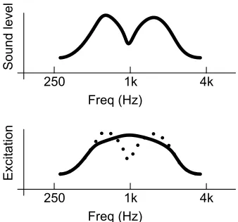
SNHL has a number of symptoms; it can cause decreases in audibility, dynamic range, frequency resolution, temporal resolution or a combination of these impairments. Decreased audibility results in sounds below a threshold not being heard. This can cause serious speech intelligibility problems, as speech is interpreted by the brain decoding the energy patterns in particular frequency ranges. Decreased audibility may mean that critical components of some phonemes are missed completely. Dillon [24] presents a good example: consider the vowels /oo/ and /ee/ which are indistinguishable by their first formant. A loss in audibility above 700Hz, masking their second and higher formant frequencies, would leave both vowels audible but sounding almost identical. Other phonemes, e.g. fricatives, would become completely inaudible. This is illustrated in Fig. 2.4.
Figure 2.4: Illustration of decreased frequency resolution as the auditory filters broaden and fail to distinguish between two independent peaks. The vowels /oo/ and /ee/ are indistinguishable by their first formant. A loss in audibility above 700Hz, masking their second and higher formant frequencies, would leave both vowels audible but sounding almost identical. (a) Input sound spectrum with two peaks; (b) excitation experienced in auditory system for normal (dotted) and SNHL impairment (solid line). Adapted from Dillon [24].
refers to the intensity range at which sound can be heard, meaning the range from the softest sound perceived to the level of discomfort. This range decreases as the threshold level increases, while the upper threshold of loudness discomfort remains static. Using simple amplification to boost the audibility above the lower threshold ensures that weak sounds are not missed. Unfortunately, this also causes sounds that would have normally been at a comfortable medium or loud range to overshoot the upper boundary and become uncomfortably loud.
Hearing aids can be used to address these problems, using amplification of the signal to counter the threshold degradation and by using limiting filters and compression to ensure the signals are within a reduced dynamic range. However, decreased frequency resolution and tem-poral resolution pose a more challenging problem.
Decreased frequency resolution is a reduction in the ability to separate and distinguish be-tween different sounds at similar frequencies. This is due to decreased sensitivity in outer hair cells and is particularly problematic in noisy situations, as the signal is interpreted as a single broad frequency response, rather than as a number of tuned frequency peaks, as in Fig. 2.4. This decreased ability to discriminate between harmonics and isolate formants, often referred to as “the cocktail party effect” [14], is problematic as it causes a reduction in speech discrimination ability.
When the inner hair cells in an area of the cochlea cease to function completely there will be no transduction of basilar membrane vibration from that region. This has been termed a “dead region” by Moore [60]. Dead regions can be described in terms of the characteristic frequencies (CFs) of the surviving IHCs and neurons that are immediately adjacent to the dead region. Basilar membrane vibration in a dead region can be detected via a spread of vibration to adjacent regions. Hence, the true hearing loss at a given frequency may be greater than suggested by the audiometric threshold at that frequency.
2.2.1 Thresholds and Audiograms
The absolute threshold is the minimum detectable level of a sound in the absence of any other external stimulus (i.e. noise). There are a number of ways of defining and measuring a subject’s sensitivity to sound. Free field measurements are usually done in a sound proof, reflection-minimisinganechoicroom with speakers presenting the stimulus to yield aminimal audible field (MAF) measurement. Real ear measurements are done using a probe microphone placed in the auditory canal while the subject wears earphones or headphones which yields a minimum audible pressure (MAP). Both MAF and MAP are absolute measurements and are plotted as an absolute threshold (dB SPL) on the vertical axis versus frequency (Hz) on the horizontal axis. These differences, along with whether a subject is tested binaurally or monaurally, are important calibration factors as they have significant impact on baseline hearing threshold.
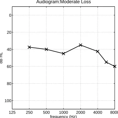
The audiogram is the common method of defining thresholds in audiology. While it can be defined in terms of an absolute threshold, it is usually specified relative to the average threshold of a young, healthy adult with unimpaired hearing. The general convention for audiograms is to specify the relative hearing level offset from the normal, in dB HL, descending on the vertical axis, and frequency in 8 octaves from 250 Hz to 8 kHz on the horizontal axis. Sometimes audiologists will also measure hearing threshold levels at half octaves: 750, 1.5, 3 and 6 kHz. An example audiogram is shown in Fig. 2.5.
2.3
Auditory Periphery Model
125 250 500 1000 2000 4000 8000 0
20
40
60
80
100
dB HL
[image:29.595.219.410.112.303.2]frequency (Hz)
Figure 2.5: Sample audiogram showing hearing thresholds for a subject with a moderate sen-sorineural hearing loss.
2.3.1 Phenomenological Models
This work used the cat AN models which were developed and validated against physiological data by Zilany and Bruce [97] and Zilany et al. [102]. The ultimate goal of the models is to predict human speech recognition performance for both normal hearing and hearing impaired listeners [100]. To date, no model claims to fully implement all the current knowledge of physiological characteristics, specifically: fibre types, dynamic range, adaptation, synchronisation, frequency selectivity, level-dependent rate and phase responses, suppression, and distortion [51]. This AN model builds upon several efforts to develop computational models including Deng and Geisler [22], Zhang et al. [96] and Bruce et al. [11]. A schematic diagram of the model is presented in Fig. 2.6. Zilany and Bruce [97] demonstrated how model responses matched physiological data over a wider dynamic range than previous models by providing two modes of basilar membrane excitation to the inner hair cell rather than one.
The design of Bruce et al. [11] modelled both normal and impaired auditory peripheries. It looked at aspects of the damage within the periphery such as inner hair cells (IHC) and outer hair cells (OHC) damage and the effects on tuning versus compression. Two-tone rate suppression and basilar membrane compression were supported and a middle ear filter was added.
The Zilany and Bruce [97] model, used in Chapter 3, built upon the previous designs and was matched to physiological data over a wider dynamic range than previous auditory models. This was achieved by providing two modes of basilar membrane excitation to the IHC rather than one. The gammatone filter was replaced by a tenth order chirp filter. The model responses are consistent with a wide range of physiological data, from both normal and impaired ears, for stimuli presented at levels spanning the dynamic range of hearing. It has been used in recent studies of hearing aid gain prescriptions [25] and optimal phonemic compression schemes [9].
The model development has continued and it has been extended and improved. In Chapter 4, their new model [102] was used, which includes power-law dynamics as well as exponential adaptation in the synapse model. Changes to the AN model, to incorporate human cochlear tuning (e.g. those used by Ibrahim and Bruce [39]), were not implemented as currently a difference in tuning between the human cochlea and that of common laboratory animals has not been definitively shown [94].
The schematic diagram of the AN model (Fig. 2.6) illustrates how model responses match physiological data over a wider dynamic range than previous models by providing two modes of basilar membrane excitation to the inner hair cell rather than one. The new power law additions are shown in the grey box.
The model is composed of several modules each providing a phenomenological emulation of a particular function of the auditory periphery. First, the stimulus is passed through a filter mimicking the middle ear. The output is then passed to a control path and a signal path. The control path handles the wideband BM filter, followed by modules for non-linearity and low-pass filtering by the OHC. The control path feeds back into itself and into the signal path to the time-varying narrowband filter. This filter is designed to simulate the travelling wave delay caused by the BM before passing through the IHC non-linear and low-pass filters. A synapse model and spike generator follow, allowing for spontaneous and driven activity, adaptation, spike generation and refractoriness in the AN. The model allows hair cell constants CIHC and
COHC to be configured, which control the IHC and OHC scaling factors and allow SNHL hearing thresholds to be simulated.
Power Law Synapse Model
Synapse Model
Spike Generator INV
NL OHC
Status C
OHC
NL
Control Path Filter CF
Chirping
C1 Filter
CF Wideband
C2 Filter
CF Middle-ear
Filter
LP LP
Σ
IHC
OHC Stimulus
Spike Times
CIHC
ƒ(τC1)
τC1
τCP
Adaptation Slow Power Law Fast
Power Law
Σ Σ
[image:31.595.97.540.88.296.2]Gaussian Noise
Figure 2.6: Schematic diagram of the AN model. Adapted from Zilany and Bruce [97]. The grey area is the additional power law module added by Zilany et al. [102] and used in Chapters 4 - 6. In this thesis, speech signals are presented as the stimulus and the output is a series of AN spike times that are used to create neurograms. The model is composed of a number of modules simulating the middle ear, inner and outer hair cells, synapse and a pseudo-random discharge spike generator.
2.3.2 Perceptual Models
Although not used in this work, other researchers have used perceptual models to predict speech intelligibility. Models such as those of Meddis [58] and Dau et al. [19] were developed with the goal of having a model that matched human perceptions. Thus, tests were carried out on humans which were then matched to the model outputs.
2.4
Neurograms
2.4.1 Speech Signal Analysis
Rosen [69] breaks the temporal features of speech into three primary groups: envelope (2-50 Hz), periodicity (50-500 Hz) and temporal fine structure (600 Hz and 10kHz). The envelope’s relative amplitude and duration are cues and translate to manner of articulation, voicing, vowel identity and prosody of speech. Periodicity is information on whether the signal is primarily periodic or aperiodic, e.g. whether the signal is a nasal or a stop phoneme. Temporal fine structure (TFS) is the small variation that occurs between periods of a periodic signal or for short periods in an aperiodic sound and contains information useful to sound identification such as vowel formants. Others [52; 77; 80] group the envelope and periodicity and refer to it as envelope (E or ENV). ENV speech has been shown to provide the necessary cues for greater than 90% phoneme recognition (vowels and consonants) in quiet with as little as four frequency bands [77], where the frequency specific information in a broad frequency was replaced with band limited noise. Cochlear implants only contain in the order of eight to 16 electrodes. They provide users with an ENV only input that lacks the finer temporal cues. This has led to recent studies focused on the contributions of ENV and TFS. Smith et al. [80] looked at the relative importance of ENV and TFS in speech and music perception, finding that recognition of English speech was dominated by the envelope while melody recognition used the TFS. Xu and Pfingst [93] looked at Mandarin Chinese monosyllables and found that, in the majority of trials, identification was based on TFS rather than ENV. Lorenzi et al. [52] suggested that TFS plays an important role in speech intelligibility, especially when background sounds are present, and that the ability to use TFS may be critical for “listening in the background dips”. They showed that hearing impaired listeners had a reduced ability to process the TFS of sounds and concluded that investigating TFS stimuli may be useful in evaluating impaired hearing and in guiding the design of hearing aids. Work by Bruce et al. [9] compared the amplification schemes of National Acoustics Laboratory, Revised (NAL-R) and Desired Sensation Level (DSL) to find an optimal single-band gain adjustment, finding that the optimal lay in the order of +10dB for envelope evaluations but -10dB to optimise with respect to TFS. The relationship between the acoustic and neural envelope and TFS was examined by Heinz and Swaminathan [34] where it was noted that envelope recovery may occur due to narrowband cochlear filtering, which may be reduced or not present for listeners with SNHL. Even though the underlying physiological bases have not been established from a perceptual perspective, current research indicates that there is value in analysing both ENV and TFS neurograms. While ENV is seen as more important for spoken English, the importance of TFS to melody, Mandarin Chinese, and to English in noise, suggests that, when looking to optimise hearing aids to increase speech intelligibility to those with SNHL both ENV and TFS restoration should be measured.
0 200 400 600 800 1000 1200 −1
0
0 200 400 600 800 1000 1200
0 0.5 1
Envelope (30−band)
0 200 400 600 800 1000 1200
−1 0 1
Time (ms)
[image:33.595.139.485.105.396.2]Temporal Fine Structure (30−band)
Figure 2.7: A sample signal, the word “ship”. The top row shows the time domain signal. Below it, the normalised envelope and temporal fine structure are presented, calculated using a 30 band filter.
where a signal,S(t), composed of N frequency bands
S(t) =
N
X
k=1
Sk(t) (2.1)
can be separated into an amplitude ENV component,Ek(t), and a TFS instantaneous phase component, cos(φk(t)), as
Sk(t) =Ek(t).cos(φk(t)) (2.2)
400 420 440 460 480 500 520 −1
0 1
Signal
400 420 440 460 480 500 520
0 0.5 1
Envelope (30−band)
400 420 440 460 480 500 520
−1 0 1
Time (ms)
[image:34.595.130.467.113.394.2]Temporal Fine Structure (30−band)
Figure 2.8: A snapshot of the previous figure showing the fricative vowel changeover time. This shows the periodic nature of the vowel captured in the ENV and the TFS with the higher frequency component of the /sh/ phoneme evident in the TFS.
2.4.2 Neurogram representations of speech
Figure 2.9: A sample signal, the word “ship”. The top row shows the time domain signal, with the time-frequency spectrogram below it. The ENV and TFS neurograms are below.
fibres were chosen to be high spontaneous rate (>18 spikes/s), 20% medium (0.5 to 18 spikes/s), and 20% low (<0.5 spikes/s). The spike train output from the AN model is used to create a post-stimulus time histogram (PSTH) with 10µs and 100µs bin sizes. Fig. 2.10 shows example PSTHs for the same fricative vowel transition shown in Fig. 2.8.
These two rates allow temporal frequency coding and average-rate intensity coding to be analysed. The PSTH is normalised to spikes per second and the frequency response of the PSTH over time is calculated as the magnitude of the discrete short-time Fourier transform (STFT), smoothed by convolving them with a 50% overlap, 32 and 128 sample Hamming window, for TFS and ENV responses respectively.
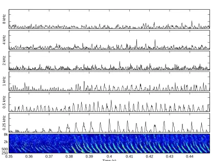
Both temporal fine structure (TFS) neurograms and average discharge rate or temporal envelope (ENV) neurograms display the neural response as a function of CF and time. The TFS neurogram retains the spike timing information showing fine timing over several microseconds; while the ENV neurogram is an average discharge rate with time resolution averaged over several milliseconds. The neurograms allow comparative evaluation of the performance of unimpaired versus impaired auditory nerves.
band in the y-axis over time in the x-axis. The fine timing information of neural spikes is retained and presented in TFS neurograms (Fig. 2.11), while the ENV neurogram smoothes the information and presents an average discharge rate using a larger bin and a wider Hamming window (Fig. 2.12). Figs. 2.11 & 2.12 illustrate how the phase-locking evident in the PSTH data at the beginning of the vowel (transition between 0.38-0.39s) is visible in the TFS neurogram but has been smoothed and averaged in the ENV neurogram.
4 kHz
2 kHz
1 kHz
0.5 kHz
0.35 0.36 0.37 0.38 0.39 0.4 0.41 0.42 0.43 0.44
0.25 kHz
Time (s)
8 kHz
4 kHz
2 kHz
1 kHz
0.5 kHz
0.35 0.36 0.37 0.38 0.39 0.4 0.41 0.42 0.43 0.44
0.25 kHz
Time (s)
8 kHz
8 kHz
4 kHz
2 kHz
1 kHz
0.5 kHz
0.25 kHz
CF (Hz)
Time (s)
0.35 0.36 0.37 0.38 0.39 0.4 0.41 0.42 0.43 0.44
[image:38.595.94.507.219.535.2]250 500 2k 8k
8 kHz
4 kHz
2 kHz
1 kHz
0.5 kHz
0.25 kHz
CF (Hz)
Time (s)
0.35 0.36 0.37 0.38 0.39 0.4 0.41 0.42 0.43 0.44
[image:39.595.106.520.229.529.2]250 500 2k 8k
F re q ( k H z ) 250 500 2k 8k C F ( H z ) 250 500 2k 8k C F ( H z ) Time (ms)
0 50 100
250 500 2k 8k P re s s u re ( P a ) Stop Time (ms)
0 50 100 150
Affricate
Time (ms) 0 100 200 300
Fricative
Time (ms)
0 50 100
Nasal
Time (ms)
0 50 100 150
SV/Glide
Time (ms) 0 100 200 300
Vowel
Input Signal
Spectrogram
ENV Neurogram
[image:40.595.94.498.113.452.2]TFS Neurogram
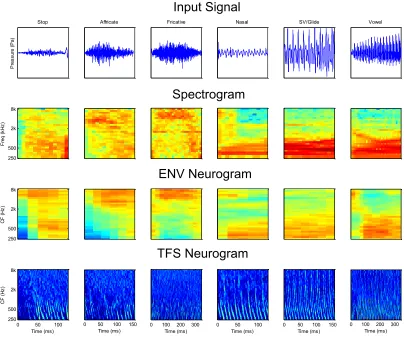
Figure 2.13: Examples of phonemes from the 6 TIMIT phoneme groupings. For each example phoneme, the pressure wave, signal spectrogram, ENV and TFS neurograms are shown. The spectro-temporal similarities can be seen between similar sounding groups, e.g. affricates and fricatives; glides and vowels. The relationship between the ENV neurogram and spectrogram is also apparent with auditory nerve activity occurring in similar characteristic frequency bands to the input signal intensity seen in the corresponding spectrogram frequencies.
2.5
Speech Perception and Intelligibility
2.5.1 Speech Perception
groups them into 6 phoneme groups: fricatives, affricates, stops, vowels, semi-vowels and glides. An example phoneme from each group is presented in Fig. 2.13. Formant transitions can be seen in the spectrograms of signals over time, as the phoneme utterance changes. An example is the difference between the spectrograms of /ba/ and /da/, where the consonant-vowel transition is differentiated by an increase in F2 frequency for /ba/ and a decrease for /da/. An example of the spectrograms are shown in Fig 2.14.
0.1 0.2 0.3 0
500 1000 1500 2000 2500 3000
Time (s)
/ba/
Frequency (Hz)
0.1 0.2 0.3 0
500 1000 1500 2000 2500 3000
/da/
Time (s)
Frequency (Hz)
Figure 2.14: Spectrograms for the sounds /ba/ and /da/. The consonant-vowel transition is differentiated between t=0 and 0.1 seconds as a small increase in F2 frequency for /ba/ and a decrease for /da/.
Speech perception relies on an interpretation of the acoustic properties of speech and the previous example illustrates how speech uses formants and formant transitions to encode both spectral and temporal cues. The mechanisms used to process this information through the auditory system and present it to the brain was covered in Section 2.1.
Speech perception is a challenge for hearing impaired listeners with difficulties in discrim-ination of speech increasing as the level of SNHL increases. While reduced audibility and an increasing speech reception threshold (SRT) are the primary problem, other factors have been the focus of research and debate for a number of decades. These are the challenges that make dealing with hearing impairment more than a question of simply “turning up the volume”.
According to Moore [61], evidence from the body of research points towards audibility as the primary factor for mild hearing losses with discrimination of supra-threshold stimuli a significant added factor for severe and profound hearing losses.
2.5.2 Quantifying Audibility
channel Speech Signal
(Tx.)
Auditory Periphery Vocal tract/
chords/mouth/ lips
brain brain
(Rx.)
(Modulate) (+Distortion/Noise) (Demodulate) (Decode)
(Encode) Idea
language language
Idea
Figure 2.15: A functional block diagram showing the transmission of an idea from a speaker to a listener. The idea is encoded via language and modulated in vocalisation. It is transmitted through a channel which distorts the signal with noise and is received via the auditory periphery when it is demodulated and presented to the brain where the language is decoded and the idea received. An AN model can be substituted for the auditory periphery, and the channel can be thought of as including this functional block, thereby assessing the noise and distortions to the signal after demodulation and presentation along the auditory nerve.
air pressure wave through the vocal chords, vocal tract and out of the mouth into a channel medium. Depending on where the speaker is situated, e.g. inside a room, a quiet environment or at a party with background babble, noise is added to the signal in the channel. The signal is received by the pinna of the listener’s ear and uses the auditory periphery to demodulate and presents the encoded signal along the auditory nerve to the listener’s brain where the signal language is decoded by the brain.
An audio signal can be corrupted in the channel by static noise. For example, additive white Gaussian noise can interfere with a signal by spectrally masking its features. Additionally, a signal can be distorted temporally by corruptions such as reverberation.
Quantitative prediction of the intelligibility of speech, as judged by a human listener, is a critical metric in the evaluation of many audio systems, from telephone channels through to hearing aids. A number of metrics have been developed to measure speech intelligibility, including static measures (AI/SII), temporal measures (STI) and measures taking account of the physiological effects of the auditory periphery (e.g. STMI and NAI, which are introduced in Sections 2.5.7 & 2.5.8). While SII and other measures have being adapted to allow prediction of speech intelligibility, due to reduced thresholds as a result of SNHL, their formulae are based on empirical findings rather than on a simulation of the impairment of the biological system. The use of a model to simulate the auditory periphery allows effects beyond the channel into the demodulation of the signal by the listener’s ear to be assessed and quantified.
2.5.3 Speech Intelligibility and Speech Quality
person for the same speech sample. One person’saveragecan be another person’s good, making it difficult to quantify consistently as the variability in the listener’s categorisation can be as large as that of the quality range. Quality also takes into account features of the speech that the listener may find annoying, e.g. too high pitched or too nasal, that influence the quality score but not necessarily the recognition or intelligibility of the speech content.
At the extreme, both quality and intelligibility rankings will converge, as a speech signal that is inaudible will rank poorly in terms of both quality and intelligibility. Correlates have been examined by Voiers [86], who gives the example of infinite peak clipping as a form of amplitude distortion that has relatively small impact on intelligibility but seriously affects the aesthetic quality of speech. It should be noted that improving quality may not positively affect intelligibility and could even reduce it, through filtering noise and impacting the speech cues at the same time, making the quality better but the intelligibility worse.
The ITU standard for speech quality assessment, Perceptual Evaluation of Speech Quality (PESQ) [40] was developed to quantify speech quality. Work to assess quality using an auditory model has also been undertaken, e.g. the Hearing-Aid Speech Quality Index (HASQI), developed by Kates and Arehart [45].
2.5.4 Speech Intelligibility Index and Articulation Index
The Articulation Index (AI) was developed as the result of work carried out in Bell Labs over a number of decades. It was first described by French and Steinberg [27] and was subsequently incorporated into the standard which is now entitled ANSI S3.5-1997 (R2007), “Methods for the Calculation of the Speech Intelligibility Index” (SII) [2]. Additions to AI mean that SII now allows for hearing thresholds, self-masking and upward spread of masking as well as high presentation level distortions.
The AI measure is described as a range from 0 to 1 or a percentage, where 1 represents perfect information transmission through the channel. As summarised by Steeneken and Houtgast [81], computing the AI consists of 3 steps: calculation of the effective signal-to-noise ratio (SNR) within a number of frequency bands; a linear transformation of the effective SNR to an octave-band-specific contribution to the AI; and a weighed mean of the contributions of all relevant octave bands. The original definition of AI summed over twenty equally spaced, with contiguous frequency bands the equal 5% contributions , Wi, is
AI = 1
20 20
X
i=1
Wi. (2.3)
importance to carrying speech information.
SII is a useful tool in predicting audibility and the calculation methodology will account for any masking of speech due to absolute hearing thresholds or noise masking. This allows the amount of information being lost to be calculated and scored as a measure of intelligibility. The SII score is not a percentage speech recognition predictor and in order to get a word or phoneme recognition score from SII, a transfer function for the specific test material or word set needs to be used. These have been calculated for several speech tests [2; 83].
2.5.5 Speech Transmission Index
Steeneken and Houtgast [81] proposed an alternative temporal metric, called the Speech Trans-mission Index (STI). Like AI, STI was developed to predict speech intelligibility loss due to channel effects and was validated for noise echoes and reverberation. It handles distortion in the time domain using an underlying Modulation Transfer Function (MTF) concept for the transmission channel. It is an indirect speech intelligibility metric as it is focused on how intel-ligibility is affected by the channel between speaker and listener. The MTF, developed for STI, was incorporated in the ANSI standard for SII.
2.5.6 Speech Intelligibility for Hearing Impaired Listeners
While SII has been shown to predict speech intelligibility for normal hearing listeners and rea-sonably well for mild hearing losses [65], it tends to over-predict at high sensation levels and under-predict for low sensation levels, especially for people with severe losses [15].
There have been a number of proposed changes to SII to allow speech intelligibility to be predicted with better accuracy for hearing-impaired listeners, e.g. [15; 67], but SII remains, fundamentally, a measure of audibility. An interesting point highlighted by Moore [61], based on the results from Turner et al. [85], is that detection of speech may not drop as quickly as intelligibility of speech because while detection requires audibility, intelligibility depends on multiple cues over a wider frequency range.
An alternative approach has been to use models of the auditory periphery to simulate the impairments that occur with SNHL as hair-cells deteriorate in performance and to measure the simulated outputs and quantify the results into an intelligibility metric.
A number of metrics have been developed to measure speech intelligibility by taking account of the physiological effects of the auditory periphery. The Perception Model (PeMo) of Jurgens and Brand [42] uses phoneme based modelling to correlate simulated recognition rates with human recognition rates. STMI and NAI also aim to predict speech intelligibility from internal representations of speech produced from AN models.
2.5.7 Spectro-Temporal Modulation Index (STMI)
to assess the effects of noise, reverberations and other distortions.
STMI can be applied directly to a transmission channel or indirectly via noisy recordings of a channel. As such, it is not a full reference measure that requires access to the channel to get a clean standard to measure against. It carries out a short term Fourier transform (STFT) and smoothing across 8 ms which puts it in the ENV category in terms of temporal resolution. The effects of TFS are not addressed. The metric is a relative mean squared error of spectro-temporal response fields between the noisy token (N) and clean template (T)
ST M IT = 1−||T−N||
2
||T||2 (2.4)
where||T−N||2 is taken to be the shortest distance between the noisy and clean token and is taken relative to the clean token reference,||T||2. The superscript T is used to emphasize that a speech template is used as the clean reference.
STI works best with separable distortions in terms of frequency and time, e.g. either static white noise which distorts across the spectral bands or reverberation which distorts temporally. STMI can deal with predictions where either or multiple distortions occur. Results were com-pared to human tests as well as STI. STMI was shown to be sensitive to non-linear distortions (e.g. phase jitter) to which simpler measures, like STI, were not sensitive.
STMI is a good example of using biologically inspired algorithms, in the form of the AN model, to predict effects in the transmission channel. It was not used in this case to predict hearing loss or to extend the channel definition to include the auditory periphery, however it shows the potential of modelling to intelligibility prediction. Bruce et al. [9] used STMI in combination with the AN model [97], to show that the metric was able to produce qualitatively good predictions of rollover in intelligibility at high presentation levels. They also measured audibility for unaided hearing impaired listeners and the effects of background noise.
2.5.8 Neural Articulation Index (NAI)
information distortion thresholds were not significantly different.
Testing was carried out with a consonant-vowel-consonant Dutch word corpus. The method-ology was restricted to simulating high spontaneous rate fibres only and it ignored the effects of neural refractoriness (i.e. the amount of time before another AN firing can occur) by using the synaptic release rate to approximate the discharge rate. NAI measures over seven octave frequency bands between 125 and 8000 Hz. These approximation restrictions to the simulation were taken to avoid having to generate many spike trains when building up estimates of discharge rates over each CF band. The neural distortion error (ǫij) for the ith frequency band and jth impaired condition is calculated as a projection of the degraded (d~) instantaneous spike discharge rate vector against the reference (~r) spiking rate vector and normalised with the reference
ǫij =|1−
~ rid~ij
T
~ rir~iT
| (2.5)
This is essentially a correlation metric that is then weighted as per band importance weighting (similar to those used in STI but calculated specifically for neural representations) and summed
N AIj =
N
X
i=1
αi·ǫi (2.6)
where αi is the band importance weighting and theǫi is from eqn. 2.5.
The metric was used by Bondy et al. [3], in a study that aimed to design a hearing aid by re-establishing a normal neural representation through a technique named neurocompensation. The input stimulus used was long term average speech shaped (LTASS) noise. As NAI is not a direct intelligibility metric, it was used to provide a relative indicator between the hearing aid strategies tested.
2.6
Image Similarity Metrics for Neurogram Comparisons
−1 0 1
Freq (kHz)
Spectrogram
0 5 10
CF (Hz)
ENV Neurogram: 65 dB SPL
250 500 2k 8k
CF (Hz)
ENV Neurogram: 30 dB SPL
250 500 2k 8k
CF (Hz)
ENV Neurogram: 15 dB SPL
Time (s)
0.1 0.2 0.3 0.4 0.5 0.6 0.7 0.8 0.9
250 500 2k 8k
Figure 2.16: A sample signal, the word “ship”. The top row shows the time domain signal, with the time-frequency spectrogram below it. Three sample ENV neurograms for the same signal presented to the AN model at 65, 30 and 15 dB SPL signal intensities are presented.
2.6.1 Mean Squared Error and Mean Absolute Error
Mean squared error (also know as Euclidean distance) is a commonly used full-reference quality metric, i.e. a test image is measured against a known, error free, original image. It measures the average magnitude of errors on a point to point basis between two images. It is a quadratic score where the errors are squared before averaging which gives a higher weighting to larger errors. Mean absolute error is a similar measure, the difference being that it is a linear score where individual differences are weighted equally.
RM AE=
P
|x(i, j)−y(i, j)|
P
|x(i, j)| (2.7)
For comparative purposes, a relative mean squared error (RMSE) can be calculated in a similar fashion as:
RM SE =
s P
|x(i, j)−y(i, j)|2
P
|x(i, j)|2 (2.8)
2.6.2 Structural Similarity Index (SSIM)
The structural similarity index (SSIM) was proposed by Wang et al. [90] as an objective method for assessing perceptual image quality. It is a full-reference metric, so as with MSE, it is measured against a known, error free, original image. The metric seeks to use the degradation of structural information as a component of its measurement, under the assumption that human perception is adapted to structural feature extraction within images. It was found to be superior to MSE for image quality comparison and better at reflecting the overall similarity of two pictures in terms of appearance rather than a simple mathematical point-to-point difference. An example is shown in Fig. 2.17 for a reference image and 3 distorted versions of the same image. Each of the distorted versions, although perceptually different when assessed by a human viewer, has an almost identical MSE score. The SSIM scores are much closer to those that might be expected from a human asked to subjectively compare the images to the reference and rank their similarity. SSIM’s ability to measure similarity in neurograms can be illustrated in the same manner. Fig. 2.18 demonstrates that a vowel neurogram, presented under a range of conditions can have comparable RMSEs. Again, a subjective visual inspection would not rank the three degraded neurograms equally, which SSIM predicts. Listening to the signals that created the neurograms and subjectively ranking them yields the same results.
The SSIM between two images, the reference, r, and the degraded, d, is constructed as a weighted function of luminance (l), contrast (c) and structure (s) as in (2.9). Luminance looks at a comparison of the mean (µ) values across the two neurograms. The contrast is a variance measure, and the structure component is equivalent to the correlation coefficient between the neurograms (r) and (d). Luminance,l(r, d), looks at a comparison of the mean (µ) values across the two signals. The contrast,c(r, d), is a variance measure, constructed in a similar manner to the luminance but using the relative standard deviations (σ) of the two signals. The structure is measured as an inner product of two N-dimensional unit norm vectors, equivalent to the correlation coefficient between the original r and d. Each factor is weighted with a coefficient
Figure 2.17: SSIM comparison of images. Original reference image and 3 degraded versions of the images which have roughly the same mean squared error (MSE) values with respect to the original image, but very different perceived quality and SSIM scores (adapted from Wang et al. [90]).
Figure 2.18: SSIM comparison of neurograms. Reference vowel ENV neurogram and three neurograms for distorted signals (+5 SNR additive white Gaussian noise, Ref - 25 dB signal in quiet, and -10 dB SNR speech shaped noise. All 3 distortions give comparable RMSE but graded results in SSIM. (NSIM is a derivative metric of SSIM which is introduced in Chapter 4 and presented here for reference.)
S(r, d) =l(r, d)α·c(r, d)β·s(r, d)γ (2.9)
S(r, d) = ( 2µrµd+C1
µ2
r+µ2d+C1
)α·( 2σrσd+C2
σ2
r+σd2+C2
)β·( σrd+C3
σrσd+C3
)γ (2.10)
![Figure 2.6: Schematic diagram of the AN model. Adapted from Zilany and Bruce [97]. The](https://thumb-us.123doks.com/thumbv2/123dok_us/1492410.689559/31.595.97.540.88.296/figure-schematic-diagram-model-adapted-zilany-bruce.webp)