Functional Coefficient Moving Average
Model with Applications to forecasting
Chinese CPI
Chen, Song Xi and Lei, Lihua and Tu, Yundong
Peking University, University of California, Berkeley, Peking
University
2014
Online at
https://mpra.ub.uni-muenchen.de/67074/
FUNCTIONAL COEFFICIENT MOVING AVERAGE MODEL WITH
APPLICATIONS TO FORECASTING CHINESE CPI
Song Xi Chen, Lihua Lei and Yundong Tu*
Peking University
Abstract: This article establishes the functional coefficient moving average model (FMA), which allows the coefficient of the classical moving average model to adapt with a covariate. The functional coefficient is identified as a ratio of two con-ditional moments. Local linear estimation technique is used for estimation and asymptotic properties of the resulting estimator are investigated. Its convergence rate depends on whether the underlying function reaches its boundary or not, and asymptotic distribution could be nonstandard. A model specification test in the spirit of H¨ardle-Mammen (1993) is developed to check the stability of the functional coefficient. Intensive simulations have been conducted to study the finite sample performance of our proposed estimator, and the size and the power of the test. The real data example on CPI data from China Mainland shows the efficacy of FMA. It gains more than 20% improvement in terms of relative mean squared prediction error compared to moving average model.
Key words and phrases: Moving Average model, functional coefficient model, fore-casting, Consumer Price Index.
1
Introduction
Autoregressive Integrated Moving Average (ARIMA) models have been pop-ular in time series analysis due to the simplicity and adaptability. An ARIMA(p, d, q) model has the following expression:
(1−B)d(1−φ1B− · · · −φpBp)xt=µ+ (1 +θ1B+· · ·+θqBq)ǫt
where B is the lagged operator and {ǫt} is a white noise series with zero mean
and finite variance. On the one hand, it describes a special dependence structure
of data while on the other hand it can be regarded as an approximation to all stationary process according to Wold Decomposition Theorem. In the past decades, numerous works in statistics and econometrics have been devoted into studying and extending the ARIMA model and its applications (to cite a few, Box and Jenkins, 1970; Box and Tiao, 1975; Dahlhaus, 1989; Cleveland and Tiao, 1976 ; Granger and Joyeux, 1980; Hannan and Deistler, 1988; Engle and Granger, 1987).
One important application of ARIMA model is to forecast Consumer Price Index (CPI). The growth rate of CPI can be regarded as a proxy of inflation rate, which is a chief target of macro-economic management by various governments and is animportant economic indicator for investors. One pop-ular model for the CPI is ARIMA(0,1,1) (Nelson and Schwert, 1977; Schwert 1987; Barsky 1987) :
(1−B)xt=µ+ (1−θB)ǫt
where {xt} represents logarithm of CPI. Although the model is easy to
imple-ment, it puts rather stringent restrictions to the inflation dynamics that the autocovariance should be constant over time. However, it is observed for the US data that the estimates of θ are not stable over time and are fairly volatile. Stock and Watson (2006) interpreted this instability as the variation of variance, which changes inversely with the magnitude of MA coefficient estimates. The parameter instability is also observedin our analysiswhen analyzing monthly CPI data of China Mainland from January 1990 to March 2014. We build the ARIMA(0,1,1) model on the year-on-year CPI monthly growth data, and esti-mate theMA coefficientθ on an expanding window basis and a rolling window basis with a 60-monthwindow-width. These estimates are plotted in Figure 1. It can be seen that the estimates of θare quite variable.
Based on the above observations, we consider an extension of ARIMA(0,1,1) model in which the MA coefficient is a smooth function of a statecovariate zt
such that
(1−B)xt=µ+ (1−θ(zt)B)ǫt. (1)
This model is called Functional Moving Average (FMA) model of order 1, or
ma1_ma.pdf ma1_ma_roll.pdf
Figure 1: Estimates ofθon an expanding window basis (panel (a)) and a rolling window basis (panel (b))
FMA(1). The co-state variable zt contains information that affects the
dynamics of xt, and does not has to be exogeneous. The dynamic
ad-missible to zt is very general as indicated by the Assumption A3-A5
given in Section 2.2. We provides a testing procedure that determines whether a given variable is qualified as co-state variable which can be
used to improve the inference and prediction of xt in Section 2.4. In
this paper, we focus on inference on FMA(1). The extension to higher order FMA
will be discussed later in the conclusion section. The choice of zt can be
made based on, for example, related economic theory, or through a data driven procedure. In this paper, we develope a test procedure to check if a variableztis
adequate to function as a co-state variable. We note that our FMA model is related to the state-dependent models of Priestley (1980) and the autoregressive functional moving average (ARFMA) model of Wang (2008), where the latter is a specific form of the former. However, the ARFMA model has the functional coefficient of the MA parts being functions of the legged values of the state variabe xt itself. Our FMA
framework has the functional coefficient depends on a co-variable zt,
with multivariate state variables. In any case, the asymptotic proper-ties of the estimators for the state-dependent and the ARFMA models have yet to be made. And we provide such results in this paper for the FMA(1) model.
In econometrics and time series literatures (Hamilton, 1994), the MA coef-ficients are often explained as the Impulse Response (IR). To be precise, for any series xt that can be written in a MA(∞) form:
xt=µ+ X
j≥0
θjǫt−j,
the j-th order IR is ∂xt
∂ǫt−j
=θj for any j ≥0. It measures the effect of a shock
on the response after j periods. For FMA(1) model, the 1-st order IR is θ(zt),
which is a function of the state variable rather than a constant as in the MA(1) model. This flexibility brings closer linkage to the real world as the effect of a shock is often affected by the state of the world.
Our work is closely related to a large body of literature on varying coefficient models. They have been well developed in nonparametric statistics and time series analysis, including ARCH/GARCH (Engle, 1982; Bollerslev, 1986), TAR (Tong, 1983; Chan and Tong, 1986; Tong, 1990; Tiao and Tsay, 1994; Caner and Hansen, 2001), EXPAR (Haggan and Ozaki, 1981; Ozaki, 1982) and FAR (Chen and Tsay, 1993; Cai, Fan and Li, 2000; Fan, Yao and Cai, 2003). This literature focuses mainly on extending the AR component of the ARIMA model, while the current work aims to relax the flexibility of the MA component. See also Priestley (1980) and Wang (2008).
The unique feature in the inference for the FMA(1) model is the esti-mation technique. Unlike the FAR(1) model which has a regression form, local polynomial regression cannot be directly applied to FMA (1). Nevertheless, we find that the functional coefficient is identified via the conditional autocovariance function. As a result, the functional coefficient can be consistently estimated by first estimating the autocovariance function. To this end, local linear least square is used to obtain estimates of conditional moments.
dependence structure. Second, the FMA(1) model could also be generalized to allow for multiple state variables Zt. To avoid the curse of dimensionality, a
single index structure forθ(·), such asθ(Zt⊤γ), could be imposed and estimation procedure adapted from Ichimura (1993) can be used. Nevertheless, the identifi-cation and estimation technique proposed in this paper would not simply apply in either case. We leave these complicated extensions for future research.
The rest of paper is structured as follows. The next section introduces the details for identification and estimation of the FMA model. The asymptotic distribution of the proposed estimator is established and a model specification test is also developed. Section 3 presents simulation results that evaluate the finite sample performance of our estimator, and the size and power of the model specification test. Section 4 shows the efficacy of FMA model by forecasting Chinese CPI data and compare it to MA(1) models. Section 5 concludes with remarks on future work. All technical lemmas and proofs are left in the appendix.
2
Theoretical Property
2.1 Identification and Estimation
For MA(1) model
xt=µ+ǫt+θǫt−1
where {ǫt} is a white noise process with variance σ2, the variance and the first
autocovariance ofxt is
E((xt−µ)2) = (1 +θ2)σ2,
E((xt−µ)(xt−1−µ)) =θσ2.
Higher order autocovariances are all 0’s. Thenθcould be estimated via the ratio of two moments after certain transformation.
Now suppose that xt follows a FMA model with the state variablezt, i.e.
xt=µ+ǫt+θ(zt)ǫt−1.
|θ(zt)| ≤ 1. Conditional on zt, its autocovariance functions follows a similar
structure as those of MA(1). To see this, it follows from the definition that
E((xt−µ)2|zt=z) =E(ǫ2t|zt=z) + 2θ(z)E(ǫtǫt−1|zt=z) +θ2(z)E(ǫ2t−1|zt=z)
E((xt−µ)(xt−1−µ)|zt=z) =E(ǫtǫt−1|zt=z) +E(θ(zt−1)ǫtǫt−2|zt=z)
+θ(z){E(ǫ2t−1|zt=z) +E(θ(zt−1)ǫt−1ǫt−2|zt=z)}.
If forj, k= 0,1,
E(ǫt−kǫt−j|zt) =E(ǫt−kǫt−j) =σ2I(j=k) and (2)
E(ǫt−jǫt−2|zt, zt−1) =E(ǫt−jǫt−2) = 0, (3) then
E((xt−µ)2|zt=z) = (1 +θ2(z))σ2 and (4)
E((xt−µ)(xt−1−µ)|zt=z) =θ(z)σ2. (5)
Now the two conditional moments have the same form with those of the MA(1) model. The condition (2) and (3) are satisfied if (zt, zt−1) is independent of (ǫt, ǫt−1, ǫt−2) for all t. In practice, zt is often taken as lagged variables (e.g.,
xt−d, for somed >2) that contain the state information, as in FAR (Cai, Fan and
Yao, 2000). This requirement is not as stringent as it appears, since it is often reasonable in application to assume the independence between the future innova-tions and the past variables. This condition is precisely described in Assumption (A5) below.
Nonparametric method of moments can be used to estimate θ(z). To do so, we need to estimate two conditional moments (4) and (5). Many nonparametric estimators could be used such as the Nadaraya-Watson estimator (Nadaraya, 1964; Watson, 1964) and the local polynomial estimator (Fan and Gijbel, 1996). We prefer to using the local linear estimators due to its attractive statistical properties including the minimax efficiency, automatic boundary correction and a simpler form of the asymptotic bias. Denote the local linear estimator of the
variance and the autocovariance by ˆa0(z) and ˆa1(z), i.e.
(ˆaj(z),ˆbj(z)) =argmin(a,b)
T X
t=1
{(xt−x¯)(xt−j −x¯)−a−b(zt−z)}2K(
zt−z
h ),
for j = 0,1, where ¯x = T−1PTt=1xt is a consistent estimator for µ, k(·) is a
kernel function andh is the smoothing parameter.
Denote g(w) = w/(1 +w2), which is monotone in w ∈ [−1,1]. A natural estimator for g{θ(z)}is
ˆ
g{θ(z)}= ˆa1(z) ˆ
a0(z)
. (6)
Note that |g(w)| ≤ 1/2 for all w ∈ [−1,1]. To incorporate this restriction, we consider the constrained estimator
˜
g{θ(z)}= ˆg{θ(z)}I(|gˆ{θ(z)}| ≤ 12) + 12I(ˆg{θ(z)}> 12)−12I(ˆg{θ(z)}<−12). (7)
Then,θ(z) can be estimated by
ˆ
θ(z) =h(˜g{θ(z)}),
whereh: [−1/2,1/2]→[−1,1], and
h(x) =g−1(x) =
(
1−√1−4x2
2x ( if x6= 0);
0 ( if x= 0).
It is noted that our estimation for g(θ(z)) is based on a ratio estimator and may not be efficient. Therefore, efficient estimator for θ(z) may be constructed, which is left for further investigation.
2.2 Large Sample Theory
To maximize the clarity of presentation, we only consider the case where zt
is a scalar. The extension to allow for multi-dimensional state variables follows in a similar fashion and is further remarked in the conclusion. The following regularity conditions are assumed to obtain the large sample properties.
(A1) h=O(Tǫ0−1) as T → ∞for someǫ
(A2) The kernel function K(·) is symmetric and Liptchitz on its supportSK =
[−1,1], in that there exists a M > 0 such that |K(x)−K(y)| ≤ M|x−y|
for allx, y∈SK.
(A3) (i) {ǫt} is a white noise sequence with Eǫ2t = σ2 < ∞, E|ǫt|2δ < ∞ for
someδ > 2; (ii) {ǫt, zt} is a strictly stationary α-mixing process with the
mixing coefficients satisfying the condition α(k) < ck−β for some β >
max{2δδ−−22,2−ǫ0ǫ0} and constantc >0.
(A4) (i) The density functionp(z) ofzthas a bounded second derivative; (ii) the
conditional density function of (z1, zm) given (x1,· · · , xm) is bounded by a
C0 >0 uniformly withm≥0; (iii) the conditional density ofxt given zt is
continuous.
(A5) (i) For eachtandj, k= 0,1,E(ǫt−kǫt−j|zt) =σ2I(j=k) andE(ǫt−jǫt−2|zt, zt−1) = 0; (ii) E(|ǫt−j|2δ|zt = z) ≤ M < ∞ for some M and j = 0,1,2, and the
sameδ in (A2).
(A6) The coefficient functionθ(z) has continuous second derivative and|θ(z)| ≤ 1 for anyz∈R.
Conditions (A1) and (A2) are standard assumptions in the kernel smooth-ing literature. For instance, the second-order Epanechnikov kernel satisfies this requirement and is used throughout the paper. Conditions (A3) and (A4) are used by Masry and Fan (1997) for α-mixing processes. The condition imposed on β in (A3) is a technical requirement. If ǫt satisfies the Cram´er Condition,
i.e. Eeλ|ǫt|α < ∞ for someλ, α > 0, then δ can be arbitrarily large and hence
(A3) can be reduced toβ >2 if ǫ0 > 23. Condition (A5.i) is needed for identifi-cation of the model, which has been discussed in the last subsection. (A5.ii) is a technical condition in order to apply the result of Masry and Fan (1997). It holds under (A3) if zt is independent of (ǫt, ǫt−1, ǫt−2). (A6) places smoothness condition on the functional coefficient. We note that In particular, zt does
not have to be exogeneous. The dynamic admissible to zt is very
We begin with the asymptotic normality of ˆg{θ(z)}. The following quantities are needed to present the asymptotic distribution of ˆg{θ(z)}. Let
G(z) = u(z)⊤Au′′(z) 2[1 +θ2(z)]2σ
2
K, ν(z) =
u(z)⊤Γ(z)u(z)
[1 +θ2(z)]4p(z)R(K), A=
0 −1 1 0
!
, and
Γ(z) =Cov
(xt−µ)(xt−1−µ),(xt−µ)2|zt=z/σ4,
where σK2 =R
u2K(u)du, R(K) = R
K2(u)du, u(z) = (1 +θ2(z),−θ(z))⊤, and
θ′(z) andθ′′(z) are the first and second derivatives ofθ(z). LetS={z|p(z)>0}.
Theorem 1. Under Assumptions (A1)∼(A6), it holds forz∈Sthat as T → ∞,
√
T h(ˆg{θ(z)} −g{θ(z)} −G(z)h2)−→d N(0, ν(z)).
Remark 1. Let M={z:θ(z) = ±1}. Since |θ(z)| ≤1 for all z ∈R, the points
inMare local extremas ofθ(z). Thus,θ′(z) = 0 for allz∈M. It is easily shown
thatG(z) = 0, forz∈M.
The next theorem establishes the asymptotic property of ˜g{θ(z)}, the con-strained estimator ofg{θ(z)}.
Theorem 2. Under Assumptions (A1)∼(A6), it holds forz∈S that
(i) If|g{θ(z)}|< 12,
p
T h/ν(z)(˜g{θ(z)} −g{θ(z)} −G(z)h2)−→d Φ;
(ii) Ifg{θ(z)}= 12,
p
T h/ν(z)(˜g{θ(z)} −g{θ(z)})−→d Φ−;
(iii) Ifg{θ(z)}=−12,
p
T h/ν(z)(˜g{θ(z)} −g{θ(z)})−→d Φ+,
where Φ is the standard normal distribution function, and
The above theorem reveals the distribution discontinuity at the bound-aries of g{θ(z)}. Intuitively, when |g{θ(z)}| < 1/2, the unconstraint estima-tor ˆg{θ(z)} will be the same as ˜g{θ(z)} for sample size large enough. There-fore, the unconstraint estimator and the constraint estimator are asymptotically equivalent. However, when |g{θ(z)}| = 1/2, the constraint becomes binding, i.e. ˆg{θ(z)} 6= ˜g{θ(z)}, with positive probability. In this case, the asymptotic distribution of the constrained estimator will be different from that of the un-constrained one.
Now we are in a position to state the asymptotic property of ˆθ(z) =h(˜g{θ(z)}). Note thath(x) is differentiable when|x|<1/2. The delta-method can be applied to Theorem 2 to obtain the asymptotic distribution of ˆθ(z). At |x| = 1/2, the asymptotic distribution can be derived directly. See the appendix for details.
Theorem 3. Under Assumptions (A1)∼(A6), it holds forz∈S that
(i) If|θ(z)|<1,
p
T h/ν(z)g′{θ(z)}(ˆθ(z)−θ(z)−g′{θ(z)}−1G(z)h2)−→d Φ;
(ii) Ifθ(z) = 1,
4 p
T h/ν(z)(ˆθ(z)−θ(z))−→d HΦ−;
(iii) Ifθ(z) =−1,
4 p
T h/ν(z)(ˆθ(z)−θ(z))−→d HΦ+,
whereHΦ−(x) = Φ(−x2/4)I(x <0) +I(x≥0) and HΦ+(x) = Φ(x2/4)I(x≥0).
It is seen that the convergence rate of ˆθ(z) depends on whether |θ(z)|<1. Whenθ(z) =±1, it converges at a slower rate and its asymptotic distribution is nonstandard.
We note that asymptotic variance of the above estimators rely on the un-known parameter σ2. It could be consistently estimated by the sample average of the squared innovation residuals ˆǫ2
t, fort= 1,· · ·, T under Assumption (A3),
where ˆǫtcould be obtained in a similar iterative procedure like that in the moving
2.3 Bandwidth Selection
The theoretical optimal bandwidth for estimatingθ(z) minimizing the asymp-totic mean squared error of ˆθ(z) can be shown as
ˆ
hopt = (ν(z)g′(θ(z)) 2 4G(z)2T )
1 5 =
cK
u(z)⊤Γ(z)u(z)g′(θ(z))2
u(z)⊤Λ(z)u(z)p(z)
1 5
T−15 (8)
where cK = R(K)/σK4 and Λ(z) =
0 −1 1 0
!
u′′(z)u′′⊤(z) 0 −1 1 0
!
. This
theoretical optimal bandwidth depends on the unknown elements θ(z), Γ(z), Λ(z) and p(z). In practice, these terms can be estimated consistently with a prior bandwidth.
A practical way of bandwidth selection is to adopt the Residual Squares Criterion (RSC) proposed by Fan and Gijbel (1995), which avoids the above complication. Let
ˆ
Γ(z, h) = 1 ∆
T X
t=2
(Yt−Yˆt)(Yt−Yˆt)⊤K(
zt−z
h )
where ∆ = tr(W −W Z(Z′W Z)−1Z′W), Z = [(1, z2 −z)⊤, . . . ,(1, zT −z)⊤]⊤,
W = diag{K(z2h−z),· · · , K(zT−z
h )}, Yt = ((xt−µ)2,(xt−µ)(xt−1 −µ))⊤ and
ˆ
Yt= (ˆa∗0(zt),ˆa∗1(zt))⊤, where
(ˆa∗j(z),ˆb∗j(z)) =argmina,b T X t=1
{(xt−µ)(xt−j−µ)−a−b(zt−z)}2K(
zt−z
h ).
With the similar arguments of Fan and Gijbel (1995), it can be shown that
E(ˆΓ(z, h)|z2,· · · , zT) = Γ(z) +dKΛ(z)h4+op(h4) (9)
wheredK =R u4K(u)du−σK4 .
As a result, our criterion for bandwidth choice is defined as
R(z, h) =u(z)⊤Γ(ˆ z, h)u(z)(1 +g′(θ(z))2V), (10)
the minimizer of R(z, h) as ¯h. Following Fan and Gijbel (1995), one can show thatadjK¯h offers a reasonable approximation for ˆhopt in practice, where
adjK =
4cKdK
R(K)
15
= 415 R
u4K(u)du
R
u2K(u)du2 −1 !15
.
To see this, by Fan and Gijbel (1995), we have
V = R(K)
T hp(z)(1 +op(1)). (11) In addition, it follows from (10) and (11) that
E(R(z, h)|z2,· · · , zT) =u(z)⊤Γ(z)u(z) +dKu(z)⊤Λ(z)u(z)h4
+R(K)u(z)
TΓ(z)u(z)g′(θ(z))2
T hp(z) +op(h 4+ 1
T h).
It can be shown that the minimizer of the leading term of the above expression is
ˆ
ho = ˆhopt/adjK.
Note thatR(z, h) depends on the unknownθ(z), we can use ˆθ(z) with a prior bandwidth h to replaceθ(z). Furthermore, the constant adjK is determined by
the chosen kernel function. For example,adjK = (92/7) 1
5 for the Epanechnikov
kernel.
To obtain a globally optimal bandwidth, one can minimize
IR(h) =
Z
R(z, h)dz
and useadjK·argminhIR(h) as the bandwidth. For implementation, the integral
can be approximated by a discrete summation over the observed data. Finally, we note that undersmoothing is often desired as one would like to avoid the bias estimation in practice.
2.4 Model Specification Test
On the other hand, when the underlying model is not an MA(1) model but an FMA model, using a misspecified an MA(1) model can produce erroneous infer-ence. Therefore, a model specification test is needed to check if the specification of FMA model is adequate.
Various approaches can be taken to construct such a specification test, for example, following Fan and Li (1996) or Chen and Gao (2007) among others. We are to adopt the L2 norm based test for regression functions (degenerated to a parameter in our case) proposed by H¨ardle and Mammen (1993) for testing the constancy of θ(z), due to its simple nature in implementation. The null hypothesis is
H0 :P(θ(z)≡θ for someθ∈R) = 1, while the alternative is
H1 :P(θ(z)≡θ for someθ∈R)<1.
Similar to H¨ardle and Mammen’s approach, we consider the following statistic:
DT =T h1/2 Z
R
(ˆθ(z)−θˆ)2π(z)dz
where ˆθ is maximum likelihood estimator underH0. Note that our test statistic does not have a smoothing operator on the parametric part, contrasted to the original H¨ardle and Mammen’s (1993) test, as the parametric part is a degener-ated function (i.e., a constant). To approximate the finite sample distribution of
D under H0, we use the following parametric bootstrap method in the spirit of Chen and Gao (2007):
Step 1 Apply the MA(1) model to xt and obtain the estimator of the mean ˆµ,
the coefficient ˆθ and the variance ˆσ2.
Step 2 Generate a bootstrap re-sample according to x∗t = ˆµ+ǫ∗t + ˆθǫ∗t−1 for
t= 1,2,· · ·, T, where {ǫ∗t}1≤t≤T are independentN(0,σˆ2) variables and obtain an estimate ˆθ(z) based on the resample.
Step 4 Calculate
D(Ti)=T h1/2
Z
R
(ˆθ(i)(z)−θˆ)2π(z)dz, i= 1,2,· · · , B
and calculate the (1−α)-th quantile of{D(Ti)}1≤i≤B as the critical value
of the test.
For simplicity, one can setπ(z) = 1 and use the discrete sum to approximate
DT. In the next section, we will use numerical simulations to study the size and
the power of this proposed test.
Prof. Chen would add something related to the theoretical properties of the above test.
3
Finite Sample Investigation
In this section, we generate the state variableztfrom ARIMA(1,0,1) process:
(1−0.5B)zt= (1 + 0.5B)ut,
where{ut}is a Gaussian white noise. The response xt is generated according to
xt=ǫt+sθ(zt)ǫt−1
for somes∈[0,1], where{ǫt}is an Gaussian white noise that is independent of
{ut}. Three functions chosen forθ(·) are
(1) θ1(z) = 2e−z
2
−1;
(2) θ2(z) =sin(3z);
(3) θ3(z) = (e2z−1)/(e2z+ 1).
3.1 Performance of Estimation
It is known from Theorem 3 that our estimator has slower convergence rate whenθ(z) =±1. Therefore, we only consider the case whenθ(z)<1 for the finite sample study. To do so, we shrink the chosen functions by setting s= 0.8. For each choice ofθ(z) and eachT ∈ {100,200,500,1000}, we generate {(xt, zt)}t≤T
for 1000 times and obtain 1000 estimates of θ(z), the mean value of which is plotted in solid line in Figure 2 to Figure 4. The dashed line in each figure represents the true function 0.8·θ(z) and the dotted lines are the mean value plus and minus the standard deviation. It is seen that the proposed estimator provides accurate estimation in all the three specifications.
[image:16.612.164.386.294.520.2]func1_estim.pdf
Figure 2: Plot of the true function 0.8·θ1(z) (dashed lines), averaged estimates (solid
func2_estim.pdf
Figure 3: Plot of the true function 0.8·θ1(z) (dashed lines), averaged estimates (solid
lines) and the associated one standard deviation confidence bands (dotted lines)
3.2 Finite Sample Distribution
Next we approximate the distribution of ˆθ(z) by simulations. Theorem 3 indicates that the asymptotic distribution of ˆθ(z) is determined by whether the true value lies on the boundary or not. We treat these two cases sepa-rately. We set T = 100,200,500,1000. With each T, we generate a sample {(xt, zt)}t≤T for 1000 times, and obtain 1000 estimates of θ(z), denoted by
ˆ
θ(1)(z),θˆ(2)(z),· · ·,θˆ(1000)(z). Their kernel density is calculated and compared to the asymptotic distribution of ˆθ(z).
Note that when θ(z) = ±1, the asymptotic distribution function of ˆθ(z) is discrete at±1, with the size of the atom being 1/2 respectively at the origin. Even if|θ(z)|<1, there are still some estimates concentrating on±1 when the sample size is not large enough. Thus, if we use kernel density as the empirical density, there might be two peaks at−1 and 1, which is not desirable for comparison. To circumvent this annoying feature, we turn to the asymptotic conditional distribu-tion ofp
func3_estim.pdf
Figure 4: Plot of the true function 0.8·θ1(z) (dashed lines), averaged estimates (solid
lines) and the associated one standard deviation confidence bands (dotted lines)
the conditional distribution will be 2Φ(−z2/4) forz∈(−∞,0); when θ(z) =−1, the conditional distribution will be 2Φ(−z2/4) for z∈ (0,∞). We compare the kernel density of{θˆ(i)(z) :|θˆ(i)(z)|<1}, to the corresponding asymptotic distri-bution. In addition, we also compute the fraction that|θˆ(i)(z)|= 1 , as denoted by P(A). It should be close to 0 when |θ(z)| < 1 and 0.5 when θ(z) = ±1 for large enoughT.
To save space, we set s= 1 andθ(z) =θ1(z) to illustrate the findings. First, we consider the estimation of θ(z) at z0 = √log 2. It is noted that θ(z0) = 0 ∈ (−1,1). The empirical conditional density of the standardized data are plotted in Figure 5 and the probabilityP(A) is reported at the bottom of each subfigure. The bandwidth of kernel density is selected by cross validation. The red dashed line is the standard normal density and the black solid line is the kernel density. Note that two lines are close to each other even for moderate T
and P(A) decreases to 0 when the sample size becomes larger.
0.5 when the sample size increases.
[image:19.612.163.385.135.360.2]non-boundary.pdf
Figure 5: The finite sample distribution of ˆθ1(z) at z0 = √log 2 (solid lines) and the theoretical asymptotic distribution (dashed lines) together with the probability ofA=
{θˆ1(z0) =±1}
3.3 Size and Power of the Test
In this subsection, we study the size and the power of the model specification test via simulation. The size is estimated by the proportion of rejection under the null hypothesis while the power is estimated by that under the alternative. As for the size, we consider the following DGP:
xt=ǫt+θǫt−1
The coefficient θ is set to be 0.2,0.4,0.6,0.8,1.0, respectively. For each θ and each sample sizeT ∈ {100,200}, we generate 500 sets of data and calculate the proportion of rejection when the significance level α is 0.05. The results are reported in table 1. It can be seen that the test has proper size.
As for the power, we consider the following DGPs.
boundary.pdf
Figure 6: The finite sample conditional distribution of ˆθ1(z) atz0= 0 given|θˆ1(z0)|<1
(solid lines) and the theoretical asymptotic distribution (dashed lines) together with the probability ofA={θˆ1(z0) =±1}
Table 1: Rejection Rate UnderH0 (α= 0.05) T s=0.2 0.4 0.6 0.8 1.0
100 0.052 0.040 0.042 0.048 0.050 200 0.048 0.044 0.050 0.050 0.048
where j ∈ {1,2,3} and s ∈ {0.2,0.4,0.6,0.8,1.0}. For each design and sample sizeT ∈ {100,200}, we generate 100 sets of data and calculate the proportion of rejection when the significance levelαis 0.05. The results are reported in table 2 and it is seen that the rejection rate gets larger when sincreases. For moderate value of s, the power is desirable.
4
Application to Chinese CPI
[image:20.612.174.375.414.462.2]Table 2: Rejection Rate UnderH1 (α= 0.05) θ(z) T s= 0.2 0.4 0.6 0.8 1.0
θ1(z) 100 0.02 0.06 0.36 0.54 0.66 200 0.10 0.32 0.64 0.84 0.86
θ2(z) 100 0.10 0.02 0.24 0.38 0.48
200 0.06 0.14 0.26 0.60 0.74
θ3(z) 100 0.16 0.42 0.70 0.72 0.78 200 0.26 0.38 0.70 0.92 0.98
database (www.wind.com.cn). The raw data is plotted in panel (a) of Figure 7. It is clear that the data is nonstationary (the p value of ADF test is less than 0.01). The first order difference of the data is plotted in panel (b) of Figure 7.
rawdata.pdf
Figure 7: The CPI monthly growth rate (panel (a)) and its first order difference (panel (b))
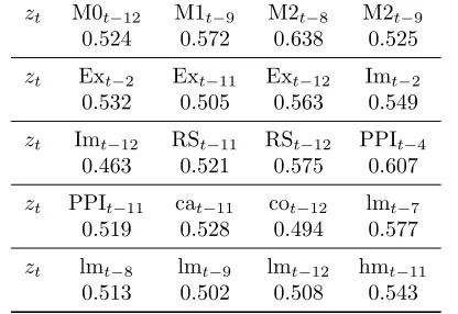
Our target is to forecast the data ranging from Jan. 2011 - Mar. 2014. If we use the MA(1) model for the first-order differenced log CPI (or equivalently, ARIMA(0,1,1) for CPI), the root mean squared forecast error (RMSE) of MA(1) model is 0.589.
[image:21.612.80.515.326.551.2]we consider are various measures of money supply, including M0, M1, M2, as the neutrality of money implies that increase in money supply will eventually convert to the increase in price level. Other economic variables which may affect the level of price includes export (Ex), import (Im), retail sales (RS) and PPI are also considered. Since PPI is often presumed to be the leading index of CPI, we also consider 4 sub-categories of PPI: capital goods (ca), consumer goods (co), light manufacturing (lm) and heavy manufacturing (hm). Year-on-year growth rate data for these 11 state variables are obtained from Wind Database. Since all variables are non-stationary, first-order differenced series are used.
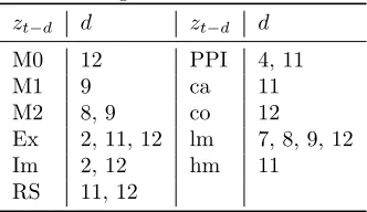
First, we conduct the model specification test to detect the state variables whose corresponding coefficient functions differ from a constant significantly. For each variable, we include lagged variables starting from the 2-nd order to the 12-th order. The 1-st order lagged variables are excluded for identification require-ments. Among all of 121 state variables (11 variables with 11 lags for each), we find that 20 of them are significant atα = 0.05. These findings are summarized in Table 3.
[image:22.612.192.358.466.562.2]Due to the space limit, we plot the estimate of θ(·) with respect to 6 of the significant variables,M0t−12,M2t−8,Ext−11,Imt−12,cot−12 and lmt−12, as illustrations in Figure 8, which displays strong departure from constancy.
Table 3: Significant State Variables
zt−d d zt−d d
M0 12 PPI 4, 11
M1 9 ca 11
M2 8, 9 co 12 Ex 2, 11, 12 lm 7, 8, 9, 12 Im 2, 12 hm 11 RS 11, 12
Table 4: Forecasting RMSE of FMA(1) with Various Variables
zt M0t
−12 M1t−9 M2t−8 M2t−9 0.524 0.572 0.638 0.525
zt Ext−2 Ext−11 Ext−12 Imt−2
0.532 0.505 0.563 0.549
zt Imt−12 RSt−11 RSt−12 PPIt−4
0.463 0.521 0.575 0.607
zt PPIt
−11 cat−11 cot−12 lmt−7 0.519 0.528 0.494 0.577
zt lmt−8 lmt−9 lmt−12 hmt−11
0.513 0.502 0.508 0.543
5
Conclusion
This paper extends the moving averaging models by allowing the MA coef-ficients to adapt with a covariate. Under parameter identification, we proposed to estimate the functional coefficient by a ratio of two conditional moment esti-mators derived from local linear least squares. The consistency and asymptotic distribution of the proposed estimators are established. A H¨ardle and Mammen type adequacy test of the constancy of the functional coefficient is also proposed. Both simulation and empirical exercises show that our proposed method perform well in finite samples.
The FMA(1) framework can be extended to the general ARFMA(p,q). Let us outline how the extension can be made via ARFMA(1,2)
xt−αxt−1 =ǫt+θ1(zt, zt−1)ǫt−1+θ2(zt, zt−1)ǫt−2 (12)
where α is the AR coefficient, and θ1(·) andθ2(·) are two MA
nonpara-metric coefficient functions which depends on (zt, zt−1) as suggested by
a referee. We have assume in (12) the mean of xt is zero to simplify
the notation. After algebraic manipulation similar to those exhibated in (3)-(4), it can be shown that
V ar(xt|zt, zt−1)−2α Cov(xt, xt−1|zt, zt−1) +α2V ar(xt−1|zt, zt−1)
Cov(xt, xt−1|zt, zt−1, zt−2)−αV ar(xt−1|zt, zt−1, zt−2)
=σ2{θ1(zt, zt−1) +θ1(zt−1, zt−2)θ2(zt, zt−1)}, (14)
Cov(xt, xt−2|zt, zt−1)−α Cov(xt−1, xt−2|zt, zt−1) =σ2θ2(zt, zt−1) and(15)
Cov(xt, xt−3|zt, zt−1)−α Cov(xt−1, xt−3|zt, zt−1) = 0. (16)
Let gj(z1, z2) =Cov(xt, xt−j|zt=z1, zt−1 =z2) for j = 0,1,2,3, g3+j(z1, z2) =
Cov(xt−1, xt−j|zt=z1, zt−1=z2)forj= 1,2,3, andg7+j(z1, z2, z3) =Cov(xt−j, xt−1|zt=
z1, zt−1 =z2, zt−2 =z3). Carrying out the local linear estimation to these
functions, and denote the estimator as ˆgk(z1, z2) for k = 0,1,· · · and 8.
Then, estimators for α is
ˆ
α=n−1Pn
t=1gˆ3(zt, zt−1) ˆ
g6(zt, zt−1),
which should be more efficient than having the estimation based on a single or a few (zt, zt−1). The estimators for θ1(z1, z2) and θ2(z1, z2)
can be obtained by solving the estimating equations based on (13) to (16). The conditions assumed for FMA(1) given in Assumptions
A.2-A.5 Section 2.2 need to be updated by replacing zt by the pair
(zt, zt−1, zt−2).
We can see that as the order of the ARFMA increases, the estima-tion procedure involves more funcestima-tions. Hence, ARFMA(p,q) models with shorter order are more useful. Indeed, one criteron one should
adapt in choosing the co-state covariable zt is that it would allows
shorter orders in the ARFMA(p,q). There are certainly more to re-serach on in future on this topics.
Acknowledgement
Statistics Bureau, Center for Statistical Science and LMEQF at Peking Univer-sity. Chen was partially supported by National Natural Science Foundation of China Grants 11131002 and G0113. Tu acknowledges support from NSFC # ... and that from the Guanghua School of Management and . This work grows out of the weekly discussion of Yandong-School of Data and an earlier draft of this paper has been Lei’s undergraduate thesis, under the supervision of Chen and Tu.
Appendix: Lemmas and Proofs
Lemma 1 (Fan and Yao, 2006). Suppose that
1. {Xt, Yt} are strictly stationary and α-mixing with Pl≥1lλ[α(l)]1− 2
δ ≤ ∞
and E{|Yt|δ|Xt=x}<∞for some δ >2 and λ >1−2/δ.
2. The conditional density fX0,Xl|Y0,Yl(x0, xl|y0, yl) ≤A < ∞ for some A > 0
and all l >0.
3. The conditional distribution of Yt given Xt = u, denoted by G(y|u) is
continuous at the point u=x.
4. AsT → ∞,h→0 and there exists a sequence of positive integers sT → ∞
and sT =o((T h)1/2) such that (T /h)1/2α(sT)→0 asT → ∞.
5. K(·) is a symetric and bounded kernel with a bounded support [−1,1] such that R
K(u)du= 1.
6. σ2(·) = V ar(Yt|Xt=·) and the density function f(·) of Xt are continuous
at the point x.
Let ˆm(x) be the local linear estimator of the conditional meanm(x) =E(Yt|Xt=
x), then √
T h( ˆm(x)−m(x)−1 2
Z
u2K(u)du m′′(x)h2)−→d N(0,σ
2(x)
f(x)
Z
K2(u)du)
Lemma 2. Supposext∼F M A(1). Forj= 0,1, Let
(ˆa∗j(z),ˆb∗j(z)) =argmin(a,b)
T X
t=1
{(xt−µ)(xt−j−µ)−a−b(zt−z)}2K(
zt−z
then under the assumptions (A1)∼(A6), it holds that
√
T h ˆa∗1(z)−(1 +θ
2(z))σ2−1
2σ2Kθ′′(z)σ2h2
ˆ
a∗0(z)−θ(z)σ2−σK2(θ(z)θ′′(z) +θ′2(z))σ2h2
! d
−
→N(0,Γ(z) p(z)σ
4R(K)).
Proof. For any v= (v0, v1)T ∈R2, letyt(v) =v0(xt−µ)2+v1(xt−µ)(xt−1−µ). Denote ˆa∗(z;v) by the local linear estimator ofE(yt(v)|zt=z) =v0(1+θ2(z))σ2+
v1θ(z)σ2, i.e.
(ˆa∗(z;v),ˆb∗(z;v)) =argmina(z),b(z)
T X
t=2
(yt(v)−a−b(zt−z))2K(
zt−z
h )
Then it is easy to show that ˆa∗(z;v) =v0ˆa0∗(z) +v1ˆa∗1(z). If we proved that √
T h(ˆa∗(z;v)−E(yt(v)|zt=z)−
1 2σ
2h2σ2
K vT
θ′′(z)
2(θ(z)θ′′(z) +θ′2(z))
!
)
d
−
→N(0,v
TΓ(z)v
p(z) σ
4R(K)).
(17)
Then Lemma 2 will be proved by Cram´er Device. Now we prove (17).
First, by Assumptions (A2) and (A3), {yt(v), zt} is strictly stationary and α
-mixing such that
E(|yt(v)|δ|zt=z)< C||v||2E(|ǫt|2δ+|ǫt−1|2δ+|ǫt−2|2δ|zt=z)<∞
and α(m)≤Am−β. Letλ= β2 −1δ, thenλ >1 sinceβ >(2δ−2)/(δ−2) and
X
l≥1
lλ(α(l))1−2δ ≤A1−
2
δ
X
l≥1
l−(1−2δ)( β
2+ 1
δ−2)<∞.
Thus, the condition 1 of Lemma 1 is satisfied.
By Assumption (A1), it holds thath =O(T−(1−ǫ0)). Let s
thensT =o((T h)1/2) and
(T /h)1/2α(sT) =O(T1− 1+β
2 ǫ0(logT)−β) =o(1).
Thus, the condition 4 of Lemma 1 is satisfied.
Further, it follows Assumptions (A4), (A5) and (A6) that the conditions 2,3,5,6 of Lemma 1 hold. Therefore, (17) is proved by Lemma 1 and hence the lemma is proved by Cram´er Device.
Lemma 3. Suppose that Assumptions (A1)∼(A6) holds. Then
|ˆaj(z)−ˆa∗j(z)|=Op(
1 √
T) (18)
Proof. First, we show that ¯x=Op(T−1/2).
T V ar(¯x) = X |j|<T
(1−|j|
T )γ(j)≤
∞
X
−∞
(1−|j|
T )γ(j)<∞.
Thus limT→∞T V ar(¯x) = P∞−∞γ(h) and then ¯x = Op(T−1/2). Let wt(z) =
K(zt−z
h )(sn,2−(zt−z)sn,1), where sn,j = PT
t=1K(zth−z)(zt−z)j, then
ˆ
aj(z) = PT
t=j+1wt(z)(xt−x¯)(xt−j−x¯)
PT
t=j+1wt(z)
, ˆa∗j(z) =
PT
t=j+1wt(z)(xt−µ)(xt−j−µ)
PT
t=j+1wt(z)
.
Notice that
|ˆaj(z)−aˆ∗j(z)| ≤ |µ2−x¯2|+|µ−x¯|
PT
t=j+1wt(z)(xt+xt−j) PT
t=j+1wt(z)
.
On the one hand,
µ2−x¯2= (µ−x¯)(µ+ ¯x) =Op(
1 √
T).
On the other hand,
PT
t=j+1wt(z)(xt+xt−j) PT
xt−j|zt=z). Let Then by Lemma 1, it is easy to prove that PT
t=j+1wt(z)(xt+xt−j)
PT
t=j+1wt(z)
=Op(1)
and hence
|ˆaj(z)−ˆa∗j(z)|=Op(
1 √
T).
Proof of Theorem 1.
Without loss of generality, we assume µ= 0. Let MT =T−1PTt=1Kh(zt−z),
ˆ
g{θ(z)} −g{θ(z)}= ˆa1(z) ˆ
a0(z) −
θ(z) 1 +θ2(z) =
ˆ
a∗1(z) +Op(T− 1 2)
ˆ
a∗
0(z) +Op(T− 1 2)
−1 +θ(θz2)(z)
= θ(z)σ 2+1
2σK2θ′′(z)σ2h2+ (T h)− 1 2A
1+Op(T− 1 2)
(1 +θ2(z))σ2+σ2
K(θ(z)θ′′(z) +θ′2(z))σ2h2+ (T h)− 1
2A0+Op(T− 1 2)
−1 +θ(θz2)(z)
=G(z)h2+ (T h)−12(1 +θ
2(z))A
1−θ(z)A0+Op(1)
(1 +θ2(z))2+o
p(1)
where the second equality follows from Lemma 3, the third quality follows from Lemma 2 and
A0
A1
!
∼N(0,Γ(z) p(z)σ
4R(K))
Then it follows from Slusky Theorem that √
T h(ˆg{θ(z)} −g{θ(z)} −G(z)h2)−→d N(0, ν(z)).
Proof of Theorem 2. For (i), by Theorem 1, it suffices to prove
p
T h/ν(z)(˜g{θ(z)} −gˆ{θ(z)})−→d 0.
For arbitraryǫ >0,
=P(|gˆ{θ(z)}|> 1
2)≤P(|gˆ{θ(z)} −g{θ(z)}|> 1
2 − |g{θ(z)}|)→0. Thus, (i) is proved. Now turn to (ii). Notice thatG= 0 wheng{θ(z)}= 12, thus by Theorem 1, we know that
p
T h/ν(z)(ˆg{θ(z)} −1 2)
d
− →Z
whereZ ∼N(0,1). Let f(x) = min{x,0}, then
p
T h/ν(z)(˜g{θ(z)} −1 2) =f[
p
T h/ν(ˆg{θ(z)} −1 2)]. Since f is continuous, by continuous mapping theorem, we have
p
T h/ν(z)(˜g{θ(z)} −1 2)
d
− →f(Z),
wheref(Z)∼Φ−. Therefore, (ii) is proved and similarly (iii) is proved.
Proof of Theorem 3. (i) is directly followed from Lemma 2 and Delta Method. Now we prove (ii) while (iii) can be dealt with in similar way. It follows Remark 1 thatG(z) = 0 whenθ(z) = 1, by Theorem 1, we know that
p
T h/ν(z)(ˆg{θ(z)} −1 2)
d
−
→N(0,1),
whereZ ∼N(0,1). For any positived, we have
P
( 4 s
T h
ν(z)(ˆθ(z)−1)≤ −r
)
=P
(
ˆ
θ(z)≤1−r
4 p
ν(z)
4 √ T h ) =P (
g(ˆθ(z))≤g(1−r
4 p
ν(z)
4
√
T h )
)
=P
(
√
T h[g(ˆθ(z))− 1 2]≤
√
T h[g(1−r
4 p
ν(z)
4
√
T h )−g(1)]
)
=P
(
√
T h[g(ˆθ(z))− 1 2]≤
√
T h[−r 2p
ν(z) 4√T h +o(
1 √
T h)]
)
=P
p
T h/ν(z)(g(ˆθ(z))− 1 2)≤ −
r2
4 +o(1)
Also, since ˆθ(z)≤1, we have
4 p
T h/ν(z)(ˆθ(z)−θ(z))−→d HΦ−.
References
Barsky, R.B. (1987). The Fisher Hypothesis and the Forecastability and Per-sistence of Inflation. Journal of Monetary Economics 19, 3-24.
Bollerslev, T. (1986). Generalized Autoregressive Conditional Heteroscedastic-ity. Journal of Econometrics 31, 307-327.
Bosq, D.(1998). Nonparametric Statistics for Stochastic Processes: Estimation and Prediction(2nd ed.). Springer-Verlag, Berlin.
Box, G. E. P. and Jenkins, G. M. (1976). Time Series Analysis: Forecasting and Control (revised edition), Holden Day, San Francisco.
Box, G. E. P. and Tiao, G. C. (1975) Intervention Analysis with Applications to Economic and Environmental Problems. Journal of the American Statistical Association 70, 70-79.
Cai, Z. and Li, Q. (2008). Nonparametric Estimation of Varying Coefficient Dynamic Panel Data Models. Econometric Theory 24, 1321-1342.
Caner, M. and B. Hansen (2001). Threshold autoregression with a unit root.
Econometrica 69, 1555-1596.
Chan, K.S. and H. Tong (1986). On Estimating Thresholds in Autoregressive Models. Journal of Time Series Analysis 7, 179-190.
Chen, R. and Tsay, R. S. (1993). Functional-Coefficient Autoregressive Models.
Journal of American Statistical Association 88, 298-308.
Cleveland, W. P. and Tiao, G. C. (1976) Decomposition of Seasonal Time Se-ries - A Model for the Census X-11 Program. Journal of the American Statistical Association 71, 581-587
Dahlhaus, R. (1989), Efficient Parameter Estimation for Self-Similar Processes.
The Annals of Statistics 17, 1749-1766.
Engle, R. F. (1982). Autoregressive Conditional Heteroscedasticity With Esti-mates of the Variance of U.K. Inflation. Econometrica 55, 251-276.
Fan, J. and I. Gijbels (1995). Data-Driven Bandwidth Selection in Local Poly-nomial Fitting: Variable Bandwidth and Spatial Adaptation. Journal of the Royal Statistical Society 57, 371-394.
Fan, J. and I. Gijbels (1996). Local Polynomial Modeling and Its Applications. Chapman and Hall.
Fan, J., Yao, Q. and Cai, Z. (2003). Adaptive varying-coefficient linear models.
Journal of the Royal Statistical Society, Series B 65, 57-80.
Fan, J. and Yao, Q. (2006). Nonlinear Time Series–Nonparametric and Para-metric Methods. Springer-Verlag, Berlin.
Fan, Y. and Li, Q. (1996). Consistent model specification tests: omitted vari-ables and semiparametric function forms. Econometrica 64, 865-90.
Granger, C. W. J.,and Joyeux, R. (1980), An Introductionto Long- Memory Time Series Models and Fractional Differencing. Journal of Time Series Analysis 1, 15-29.
Haggan, V. and Ozaki, T. (1981). Modeling Nonlinear Vibrations Using an Amplitude-Dependent Autoregressive Time Series Model. Biometrika 68, 189-196.
Hamilton, J.D. (1994) Time Series Analysis. Princeton University Press.
H¨ardle, W. and Mammen, E. (1993). Comparing nonparametric versus para-metric regression fits, The Annals of Statistics 21, 1926-1947.
Ichimura, H. (1993). Semiparametric least squares (SLS) and weighted SLS estimation of single-index models,Journal of Econometrics 58, 71-120.
Masry, E. and Fan, J.(1997). Local polynomial estimation for stationary stable processes. Stochastic Processes and Their Applications 18, 1-31.
Nadaraya, E. A. (1964). On Estimating Regression. Theory of Probability and its Applications 9(1), 141-142.
Nelson, C.R. and G.W. Schwert (1977), Short-Term Interest Rates as Predictors of Inflation: On Testing the Hypothesis that the Real Rate of Interest Is Constant. American Economic Review 67, 478-486.
Ozaki,T.(1982). The Statistical Analysis of Perturbed Limit Cycle Processes Using Nonlinear Time Series Models. Journal of Time Series Analysis 3, 29-41.
Priestley, M.B. (1980). State-dependent Models: A General Appraoch to Non-linear Time Series Analysis . Journal of Time Series Analysis, 1(1), 47–71.
Stock, J.H. and M.W. Watson (2006). Why Has U.S. Inflation Become Harder to Forecast? NBER Working Paper no. 12324.
Schwert, G.W. (1987). Effects of model specification on tests for unit roots in macroeconomic data. Journal of Monetary Economics 20, 73-103.
Tiao, G. C. and Tsay,R. S. (1994). Some Advances in Nonlinear and Adaptive Modeling in Time Series. Journal of Forecasting 13, 109-131.
Tong, H. (1983). Threshold autoregression, limit cycles and cyclical data(with discussion). Journal of the Royal Statistical Society, Series B 42, 245-292.
Tong, H. (1990). Nonlinear Time Series: A Dynamical System Approach. Ox-ford,U.K.: Oxford University Press.
Wang, H.B. (2008). Nonlinear ARMA models with functional MA coefficients.
Watson, G. S. (1964). Smooth regression analysis. The Indian Journal of Statistics, Series A26, 359-372.
Guanghua School of Management and Center for Statistical Science, Peking Uni-versity, Beijing, China, 100871
E-mail: [email protected]
School of Mathematics, Peking University, Beijing, China, 100871 E-mail: [email protected]
Guanghua School of Management and Center for Statistical Science, Peking Uni-versity, Beijing, China, 100871
M012.pdf M28.pdf
Export11.pdf Import12.pdf
[image:34.612.91.461.101.669.2]PPIco12.pdf PPIlm12.pdf
Figure 8: Estimates of θ(zt) where (a) zt=∆M0t−12; (b) zt=∆M2t−8; (c) zt=Ext−11;