The influence of uncertainties and parameter structural dependencies in distribution system state estimation

The influence of uncertainties and parameter structural

dependencies in distribution system state estimation

LIAO, Huilian <http://orcid.org/0000-0002-5114-7294>, MILANOVIĆ, Jovica V.,

HASAN, Kazi N. and TANG, Xiaoqing

Available from Sheffield Hallam University Research Archive (SHURA) at:

http://shura.shu.ac.uk/18987/

This document is the author deposited version. You are advised to consult the

publisher's version if you wish to cite from it.

Published version

LIAO, Huilian, MILANOVIĆ, Jovica V., HASAN, Kazi N. and TANG, Xiaoqing (2018).

The influence of uncertainties and parameter structural dependencies in distribution

system state estimation. IET Generation, Transmission & Distribution, 12 (13),

3279-3285.

Copyright and re-use policy

See

http://shura.shu.ac.uk/information.html

1

The Influence of Uncertainties and Parameter Structural Dependencies in

Distribution System State Estimation

Huilian Liao

, Jovica V. Milanović

, Kazi N. Hasan

, Xiaoqing Tang

1 _{Power, Electrical and Control Engineering Group, Sheffield Hallam University, Sheffield, S1 1WB, UK} 2 _{School of Electrical and Electronic Engineering, The University of Manchester, PO Box 88, Manchester, M60}

1QD, UK.

*_{[email protected]}

Abstract:This paper evaluates a number of uncertain parameters that affect the accuracy of distribution system state estimation, and ranks their importance using an efficient sensitivity analysis technique, Morris screening method. The influence of the uncertain parameters on state estimation performance is analysed globally and zonally. Furthermore the dependence structure between the critical variable and state estimation accuracy is analysed using copula to establish their relationship at different section of the bivariate space. The sensitivity of the critical parameter at different ranges is also studied and ranked using Morris screening methods to present the variation of state estimation performance when the critical variable is allocated at different sections within the feasible range. Accurate assessment of the importance of various uncertain parameters and the analysis of the dependence structure can inform power system operators which parameters will require the greatest levels of mitigation or increased monitoring accuracy in order to have satisfactory performance of distribution system state estimation.

1. Introduction

Secure operation of a power system requires proper estimate of the status of operating condition [1], which is essential for identifying potential critical operating conditions and making decision on selecting preventative measures if necessary. Given inherent measurement inaccuracies, state estimation (SE) is able to smooth out measurement errors and provide an optimal estimate of the system operating states. With the increased capability of data collection in SCADA systems, SE has been widely integrated in Energy Management Systems (EMS) for operation and management in transmission systems [2].

Proliferation of active components and changing load profiles in distribution networks are affecting the operating conditions of distribution networks which change much more frequently than ever. Simultaneously more and more functionalities developed for smart grids are highly dependent on the network state estimation. Therefore it is essential to have appropriate observability of the distribution networks in order to ensure secure and efficient network operation. This need resulted in an intensive research on SE at distribution levels, namely Distribution System State Estimation (DSSE). Different from transmission networks, the ill conditioned matrices and large number of nodes in distribution networks impose great difficulty and challenges to DSSE. Various techniques have been investigated for DSSE in literature [3], e.g., machine learning, heuristic intelligence methods and especially Weighted Least Squares (WLS) approach [1].

DSSE relies on continuous measurements and, predominantly, pseudo-measurements. Considering that measurement bias exists in each measurement, the deviation of both measurements and pseudo-measurements can appreciably affect the performance of state estimation. With the increased attention paid to the study of the influence of uncertainties on SE accuracy, a number of dedicated papers

have studied the impact of different types of measurements on the accuracy of SE in order to establish the influence of measurement accuracy on the overall estimation accuracy [4]. Analytical approach is applied to perform sensitivity analysis in [5]. In [6], WLS based SE is used to establish under which circumstance and to what extent the SE results are affected by measurement uncertainty when a minimum number of measurements is used.

2 Knowing in general the influence of uncertain

parameters is not sufficient. It would be also very useful to have the correlation and joint probability between the critical uncertain parameter and the evaluated performance indices. For instance, the uncertain parameters located in different sections of the possible range may result in very different dependence relationship with the evaluated performance index. The investigation of their dependence structure can provide more detailed information beyond the sensitivity of the variable in general. Copula theory has been widely used to construct dependence function by linking together univariate distribution functions to form a multivariate distribution function [11]. It has been widely applied in finance and economics analysis, as well as to model stochastic dependence in power system uncertainty analysis [12]. Though the aforementioned techniques are very useful for uncertainty analysis, they have not been applied for DSSE analysis. Comprehensive analysis and comparison among the uncertain parameters that affect DSSE performance are still needed.

This paper contributes to comprehensive SA in which the analysis not only provides the sensitivity of SE to uncertain parameters in general, but also identifies the SE sensitivity to parameter location in the network and to the subset of the feasible range of variation in parameter values. The uncertain parameters are critically evaluated and analysed, and copula theory is used to present accurately the sensitivity and dependence structure among different variables when solving DSSE problem. The paper justifies the necessity for and benefits of performing this deeper level of SA anlaysis and for the first time applies Morris screening method and copula theory for uncertainty analysis in DSSE. The global and zonal sensitivity analysis performed in the study is able to identify the critical parameters (i.e., which) and the critical locations (i.e., where) that should be paid more attention to, and the analysis of dependence structure and sensitivity analysis of the critical parameter within different sections of the range can facilitate the decision on required mitigation levels (i.e., how).

2. Methodology

2.1. Distribution System State Estimation (DSSE)

The three-phase state estimation problem can be defined as:

𝑬 = 𝒛 − 𝐻(𝑆) (1) where state variable S consists of three-phase voltages and voltage angles (Va, Vb, Vc, θa, θb, θc). 𝒛 is a vector of

measurements, H(S) represents a nonlinear set of measurement functions that describe the measurements in terms of state variable S. 𝑬 is a measurement error vector. The DSSE problem can be solved by weighted least squares (WLS) technique which is to minimise the equation as follows:

min𝑆[𝑧 − 𝐻(𝑆)]𝑇𝑹−1[𝑧 − 𝐻(𝑆)] (2) where R is the covariance matrix of measurement errors, i.e., the weights associated with measurement tolerance. The uncertainties/tolerance of pseudo-measurements and real measurements are taken into account by adding normally distributed errors to their actual values before being used for estimation. To account for the uncertainties, Monte Carlo simulations are used in conjunction with DSSE. In the study,

the real measurement (of voltage and power) and pseudo-measurements (of power and network parameters) have different measurement tolerances, resulting in different weights associated with different measurement errors in (2). The tolerance of pseudo-measurements (power and network parameters) is further discussed in Section 3.2. The three-phase weighted least squares (WLS) state estimator is applied to solve DSSE. Further details on DSSE can be found in [13].

2.2. Uncertainty Analysis

The uncertainty variables used for sensitivity analysis (denoted as x) are the tolerances of uncertain measurements. In the study, x represents the confidence of measurement 𝒛, and determines the deviation of the measurements from their actual values before the measurements are used as inputs to DSSE. The generation of distribution of 𝒛 based on x is discussed in Section 3.2. Parameter x also determines the weights of R in (2). Therefore x to some extent influences state estimation performance. Given 𝒙, state estimation error can be evaluated by:

𝑦(𝒙) =_𝑁1

𝑏𝑢𝑠∑ (∑

|𝑉_{𝑖,𝑎𝑐𝑡}𝑗 −𝑉_{𝑖,𝑒𝑠𝑡}𝑗 (𝐱)|

𝑉_{𝑖,𝑛𝑜𝑚}𝑗

3

𝑗=1 )

𝑁_𝑏𝑢𝑠

𝑖=1 × 100 (%) (3)

where 𝑁𝑏𝑢𝑠 denotes the total number of buses in the network.

𝑉_𝑖,act𝑗 , 𝑉_𝑖,est𝑗 and 𝑉_{𝑖,𝑛𝑜𝑚}𝑗 represent the actual, estimated and nominal voltages at phase j of bus i respectively. The objective of sensitivity analysis in this paper is to study the impact of 𝒙 on the state estimation error 𝑦(𝒙), and to find out the relationship/dependence structure between 𝒙 and 𝑦(𝒙). The application and discussion in the rest of the paper are performed surround this objective.

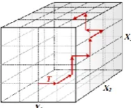
2.2.1 Morris Screening Method:Morris screening method is a randomized One-At-a-Time design. During screening procedure, only one variable changes at a time by a magnitude of Δ. The standardized effect of a positive or negative Δ change (or step) of an input variable can be evaluated by Elementary Effect (EE) defined as:

𝐸𝐸𝑖(𝒙) =[𝑦(𝑥1,𝑥2,…,𝑥𝑖−1,𝑥𝑖+∆,𝑥_∆ 𝑖+1,…𝑥𝑘)−𝑦(𝐱)] (4) where Δ is the multiple of 1/(p-1) representing the magnitude of step, p is the number of levels, k is the number of variables, and x=[ 𝑥1, 𝑥2, … , 𝑥𝑖, … 𝑥𝑘]. The Morris method creates a trajectory through the variable space by changing one variable at a time by Δ as shown in Fig. 1.

Fig. 1. Illustration of Morris screening trajectory

Each trajectory is constructed via a series of matrices [14]. r (r=p-1) trajectories are constructed, and r EEs are obtained for each input variable [7]. The finite distribution of EEs that contributed to variable i is denoted as Di. Each

Di contains r independent EEs. Based on Di the sensitivity

3 calculating the mean (𝜇∗) and standard deviation (𝜎∗) of the

set of EEs for each input variable [14, 15]:

𝜇𝑖∗=

∑𝑟𝑛=1|𝐸𝐸𝑛|

𝑟 (5)

𝜎𝑖∗= √ 1

𝑟∑ (𝐸𝐸𝑛− 𝜇𝑖)2 𝑟

𝑛=1 (6)

Index 𝜇∗ provides the overall sensitivity of the ith input variable from the perspective of the output response. Large 𝜇∗ _{suggests that the output has a high sensitivity to the input} variable. Index 𝜎∗ is used to determine the spread (variance) of the finite distribution of the EEi distribution, which

indicates the independence of the corresponding variable [8, 9]. The larger index 𝜎∗ is, the more independent the corresponding variable is. Further details about Morris screening method can be found in [8].

2.2.2 Copula Analysis and Dependence:Copula theory is able to capture the dependence between random observations and also allows the decomposition of a joint distribution into its marginal distributions and its dependence function. Consider two random observations v =[v1,v2], with joint distribution F and marginal distribution

of observations v1 and v2 (denoted as F1 and F2). The

mapping from the individual distribution functions to the joint distribution function can be defined by a copula [11]:

𝑭(𝒗) = 𝐂(𝐹1(𝑣1), 𝐹1(𝑣2)), ∀𝒗 ∈ 𝑅𝑛 (7) From any multivariate distribution F, the marginal distributions Fi can be extracted, and the copula C can be

obtained. The information contained in copula C is the information about the dependence between different variables. In this study, the copula is used to construct the dependence relationship between the tolerance of measurements and the corresponding state estimation error in order to establish whether the tolerance of measurements allocated at different sections of the possible ranges would affect the performance of the state estimation. The inputs to copula analysis are a series ofobserved 𝒙and 𝑦(𝒙), denoted as𝑣1 and𝑣2 respectively.

The copula model which fits the data the most is used to represent the structural dependence of the given data. Fitting copula models to observed data is implemented by applying widely used maximum likelihood estimation (MLE) [11,16] method. The observations are assumed to have a known probability distribution with unknown copula parameters (denoted as 𝐶𝜃). The joint probability density function F of the given observation v can be written in terms of these unknown parameters 𝐶𝜃. The copula log-likelihood function defined as (8) [16] is used to estimate the copula-based models and will attain its peak value when the unknown parameters are chosen to be closest to their actual values. Hence, MLE is actually an optimisation problem and its objective is to maximise the copula log-likelihood function (8) by varying the assumed parameters 𝐶_𝜃 of the copula models, in order to give the maximum likelihood estimates for the parameters of interest.

maximize LL=log 𝐅(𝐯; 𝐶𝜃) (8) The larger the calculated LL is, the better the estimation is.

In the study, nine widely used copulas are considered, as listed in Table 1 [16]. The notations of the unknown copula parameters 𝐶𝜃 to be estimated during MLE procedure

are also given in Table 1. The nine copulas comprise almost all of the copulas which are widely applied in statistics and economics. Among these copulas, the normal, Student’s t

and Plackett copula generate symmetric dependence, whereas the Gumbel, Clayton, and Joe-Clayton copula generate asymmetric dependence. More details on copula analysis in general, including the nine copulas used together with their copula parameters can be found in [16].

Table 1 Nine Copulas Used in the Study

Index Copula 𝐶_𝜃

1 Normal Copula 𝜌

2 Clayton's copula 𝜃

3 Rotated Clayton copula 𝜃

4 Plackett copula 𝜋

5 Frank copula 𝜆

6 Gumbel copula 𝛿

7 Rotated Gumbel copula 𝛿

8 Student's t copula 𝜌, 𝑣

9 Symmetrised Joe-Clayton copula (SJC) 𝜏𝑈, 𝜏𝐿

3. Results and Analysis

3.1. Network Settings

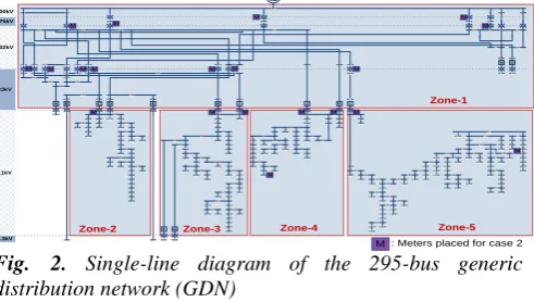
In the study, a 295-bus generic distribution network (GDN) [17] is used, as shown in Fig. 2. The GDN network was originally developed as a reference netwrok for the purpose of distribution netwrok studies in the UK, and all GDN parameters are based on realistic UK distribution networks. Unbalance phenomenon is generated by unbalanced loads [17]. The network is divided into 5 zones as marked in Fig. 2. Zone 1 consists of buses at voltage levels larger than 11kV; while zones 2-5 are allocated at 11kV level (starting from 33kV-11kV substations) and they are divided based on feeders.

24 46 17 28 16 14 12 26 21 19 23 22322 18 15 54 52 53 230 50 75 228 74 229 20 221 5176 13 268 87 48 47 49 222 43 42 41 40 39 38 37 269 235 236 231 78 79 80 81 85 88 290 82 83 84 291 91 92 93 95 94 96 97 98 10199 100 102 103104 105 106107 108 109 110 111 112 113 114115 116 121 122 123 124 125 126 127 128 117 118 119120 86 11 10 8 9 7 6 5 4 55 1 65 64 66 63 57 226 227 58 149 147 154 155 150 153 156

148 146 145 141 143 142 144 140 139 129 130 133 131 135 137136 138 134 157 161 158 186 184 132 160 165 162 163 164 166 167 168 169 170 180 181 182 183 185 187 188 189 190191 192 193 194 197 198 200199 201 202 203204 205 206 207 208 209 151 152 224 232 77 159 225 215 216 211 212 210 213 214 217 218171 219 220 172 173 174 175 176 177 178 62 60 59 61 2 3 72 70 179 25 27 29 30 32 31 33 34 35 36 71 68 67 69 73 89 45 44 249 250 266 267 242 252 260 289 237 244 261 251 241246245 243

262 272 270

253274

271276275 263 264273

240

254

258 259 256

277 247 278 248 280 234 279 233 255 257 293 292

294 295 297 296

299 298 300 77 238 288 269

287286285

56 B

A C D E

F

H I J K L

O N G 132kV 33kV 11kV 3.3kV 275kV 400kV G 195 196 Zone-1

Zone-2 Zone-3 Zone-4 Zone-5

M M M M M M M M M M M M M M M M M M M M

M : Meters placed for case 2

Fig. 2. Single-line diagram of the 295-bus generic distribution network (GDN)

The study is carried out using two different, arbitrary, sets of monitor locations for illustrative purposes. (The optimal monitor placement for state estimation is not the focus of this study). These meters provide measurements detailed in Section 3.2.

C1: Meters are placed at substations only. In total 20 meters are placed at 20 substations.

4

3.2. Uncertainties

In general, there are uncertainties associated with measurements as well as with parameters of network models. The types of real measurements and pseudo-measurements used in the study are based on [13]. Real measurements can be characterized by their own ranges of measurement errors which are primarily determined by the corresponding measurement devices [18]. The accuracy of pseudo-measurements is highly dependent on the estimation methodologies and the confidence of data resources based on which the estimation is performed. To have more accurate pseudo-measurements, various types of data in distribution networks have been explored for the purpose of DSSE [19]. Pseudo-measurements of load demand profiles, for example, can be further improved by the non-synchronized measurements coming from smart meters based on the credibility of each available measurement. The load estimation accuracy based on available data is not considered here and the SA analysis is carried out with the tolerances provided in literature.

1) Real measurements: As per IEC60044-2, there are accuracy classes 0.1, 0.2, 0.5, 1.0 and 3.0 of voltage transformers (VTs), with phase displacement ranges from 0.15 to 1.2 centiradians [20]. As per IEC61000-4-30, the measurement uncertainty of r.m.s value of the voltage magnitude ∆𝑈 for class A and B performance shall not exceed ±0.1% and ±0.5% , respectively, of the declared supply voltage by a transducer ratio respectively [21]. Combing the chain uncertainty introduced by both measurement and VTs, the range of the tolerance of voltage (U) measurements is set to [0.14%, 3.04%] [22]. The standard accuracy classes for current transformers (CTs) are 0.1, 0.2, 0.5, 1, 3 and 5, with phase displacement ranging from 0.15 to 1.8 centiradians [20]. As per IEC61000-4-30, the measurement uncertainty of r.m.s value of the current magnitude ∆𝐼 for classes A and B performance shall not exceed ±0.1% and ±2% , respectively, of the full scale [21]. Considering both VTs and CTs as well as measurement uncertainty, the range for the tolerance of power measurement is set to [0.17%, 6.16%] [22].

2) Pseudo-measurements (PMs): PMs are typically calculated using load forecasting methods or historical data. They are much less accurate than the real-time measurements and are usually assigned with low weights in

R (i.e., high error variances). For buses for which there are no data recorded, PMs of the load demand can be generated from other buses with similar types of customers. In [13, 23], 20% to 50% errors are considered in PMs. In [4], the maximum error of 50% with respect to the reference values for the active and reactive powers (P&Q) drawn by the loads is used for PMs. In [24], 10%, 30% and 50% errors are used for error of P&Q load. Generally, more information such as energy bill data and scheduled power, etc., can be used for more accurate active power estimation. Therefore it is assumed that the error of pseudo-measurement of P is smaller than that of Q.

3) Network Parameters: Loadings of the network were extracted from 2010 survey of different types of loads (including commercial, industrial and residential loads) [25]. In EN 50160, the required level of voltage unbalance factor is limited by 2% for 95% of the week in low and medium

voltage distribution systems [26]. It can be expected that negative sequence component of the supply voltage shall be within the range 0%–2% of the positive sequence component. In some areas, unbalances up to about 3% at three-phase supply terminals may occur [4]. The tolerance of the line impedances could change from zero to 20 % [27]. In [28], the tolerance of short-circuit impedances for transformers is 7.5%-15% of the declared values. In [29] the variation of OLTCT impedance due to the tap changing is found to be between 10%-15% of its nominal value. Based on the statistics given above, the ranges of uncertainty variables are set as listed in Table 2.

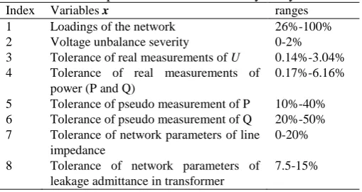
Table 2 List of input variables for sensitivity analysis

Index Variables x ranges

1 Loadings of the network 26%-100%

2 Voltage unbalance severity 0-2%

3 Tolerance of real measurements of U 0.14%-3.04%

4 Tolerance of real measurements of

power (P and Q)

0.17%-6.16%

5 Tolerance of pseudo measurement of P 10%-40%

6 Tolerance of pseudo measurement of Q 20%-50%

7 Tolerance of network parameters of line

impedance

0-20%

8 Tolerance of network parameters of

leakage admittance in transformer

7.5-15%

4) Transfer from tolerance to standard deviation: For a given percentage of the maximum allowed deviation (i.e., tolerance) from the mean 𝜇, as given in Table 2, the standard deviation of the measurement error can be derived based on 𝜎 =𝜇×%error_3×100 [23]. For each setting of variable x, the measurements (i.e., the input to DSSE) for Monte Carlo simulations are generated based on PDF(𝜇, 𝜎) with 3-sigma.

It should be mentioned that DSSE, Morris screening method and copula estimation have their own different inputs. For instance, the inputs to DSSE are the

measurements. The inputs to Morris screening method are uncertainty/tolerance of measurements i.e., the uncertainty variables listed in Table 2, denoted as 𝒙. The inputs to copula analysis are the observations of 𝒙 and 𝑦(𝒙) calculated from (3), denoted asv.

3.3. Sensitivity Analysis through Morris Method

5 distribution. Variables with low values of 𝜇∗ are considered

as non-influential and have negligible impacts on the DSSE results. From the perspective of monitoring reinforcement for the purpose of DSSE, therefore, the focus should be placed on the analysis and improvement of the accuracy of influential variables (i.e., the critical uncertainty variables).

Morris screening method is also applied to case 2, and the results are presented in Fig. 3 (b). For all variables (except for variable 3), the 𝜇∗ and 𝜎∗ of the EEs obtained in case 2 are greatly reduced compared with the results of corresponding variables in case 1. It suggests that in case 2 the uncertainty variables (except for variable 3) become less influential on DSSE performance compared with the case 1. The ranking of the variables is similar as in case 1, except that the variable 3 moved from the 4th to the 2nd place in terms of importance. The 𝜇∗ of EEs of variable 3 (i.e., the tolerance of real measurement of U) is increased from 0.29% to 0.38%, which suggests that variable 3 becomes more influential when the meter placement is given as case 2.

a b

Fig. 3. 𝜇∗ and 𝜎∗ of the EEs of various uncertain parameters

(a) Case 1, (b) Case 2

The variable ranking based on Morris method for case 2 is 1>3>2>7>8>4>5>6. Variables 4 and 8, and 5 and 6, have very similar 𝜇∗, as shown in Fig. 3(b). The Pearson correlation coefficient [10] is used to rank the importance of variables for case 2 and compared with Morris method. With the same number of simulations as Morris method, the Pearson approach generates the ranking of 1>3>2>5>8>7>6>4, i.e., similar but not exactly the same as Morris method. When the number of Monte Carlo simulations is increased to 500, the ranking is changed to 1>3>2>7>4>8>5>6, i.e., almost exactly the same as Morris method (only the rank of variables 8 and 4 was swapped). It can be seen that with increased number of simulations, the Pearson approach yields almost exactly the same results as Morris method, which demonstrates the efficiency of Morris method, as discussed in Section 1.

EE presents the change/variation of state estimation error when one variable changes at a time, and it does not present the accuracy (or error) of the state estimation with a set of given measurements. To present state estimation accuracy, further simulation is carried out as follows. The uncertainty variable 𝒙 (as given in Table 2) is set to a number of values evenly distributed within the pre-defined range, and other variables are set to base values. Given 𝒙,

estimation errors 𝑦(𝒙) are obtained by performing DSSE. For each variable in Table 2, the mean and maximum of the obtained set of 𝑦(𝐱) are calculated and provided in Table 3, in which Yμ and Ymax denote the mean and maximum of 𝑦(𝐱)

respectively. Yμ and Ymax represent the state estimation

performance rather than the variation of state estimation performance as presented by Morris screening method. It can be seen that the state estimation errors obtained in case 2 are on average 31% smaller than those obtained in case 1. As discussed in Section 3.2, the 𝜇∗ of EEs of variable 3 in case 2 is increased compared to case 1. This can be also reflected in Table 3 by the fact that the difference between

Yμ and Ymax is larger in case 2 (0.18%) than in case 1

(0.14%). Although variable 3 becomes more influential and sensitive in case 2, case 2 actually outperforms case 1 in terms of state estimation accuracy, given the same settings of variable 3. It can be seen from Table 3 that case 2

improves the estimation performance by 11.54% (0.52−0.46

0.52 ×

100) compared to case 1.

Table 3 State Estimation Error (Yμ and Ymax) for Variables in

Table 2

Case Index 1 2 3 4 5 6 7 8

1 Yμ (%) 0.89 0.64 0.52 0.46 0.46 0.45 0.45 0.43 Ymax(%) 1.43 0.94 0.66 0.51 0.48 0.49 0.55 0.48

2 Yμ(%) 0.61 0.37 0.46 0.31 0.30 0.32 0.31 0.31 Ymax(%) 0.92 0.49 0.64 0.33 0.33 0.33 0.35 0.33

Case 2 is selected for further analysis in this study due to its accurate state estimation results. As presented in Section 3.2, the top two sensitive parameters in case 2 are variables 1 and 3. The focus therefore should be on the improvement of these variables when developing mitigation strategy. Between the two variables, variable 1 cannot be reinforced as the loading of the network is highly dependent on customers’ behavior, and in practice it cannot be arbitrarily controlled by DNOs or other stakeholders in the network. As for the tolerance of real measurement of voltage U, i.e., variable 3, it could be improved by the enhancement of measurement devices.

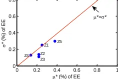
Fig.4.𝜇∗ and 𝜎∗ of the EEs of parameter 3 at five different zones

It is not feasible though, to replace the measurement devices at all monitoring locations in the network. It would be useful and cost efficient if the analysis can show in which zone of the network the accuracy of variable 3 has greater influence on the accuracy of DSSE. For this purpose, the Morris screening method is applied to rank the variable 3 in different zones (in total five zones), and the results are presented in Fig. 4. It can be seen that the tolerance of real measurement of U in zone Z5 has the largest influence on the accuracy of DSSE compared to measurementsof U in other zones. Therefore, the improvement of the accuracy of measurement of U should be attempted in zone Z5. To demonstrate the effectiveness of the zone-based uncertainty mitigation, the VTs in zone Z5 are changed from class 3 to 0.5 (with measurement performance of class A), and the measurement tolerance of U in other zones is kept at base value. By doing this the accuracy of state estimation

0 0.2 0.4 0.6 0.8 1

0 0.2 0.4 0.6 0.8

* (%) of EE



*

(%

)

o

f

E

E

1 2

7 3 8 5

4 6

*=*

0 0.2 0.4 0.6 0.8 1

0 0.2 0.4 0.6 0.8



*

(%

)

o

f

E

E

* (%) of EE

1 3 2 7 4

8 5 6

*=*

0 0.2 0.4 0.6 0.8 1

0 0.2 0.4 0.6 0.8



*

(%

)

o

f

E

E

* (%) of EE

Z1 Z5 Z2 Z3 Z4

6 improved by 37.5% (0.48−0.30

0.48 ), which demonstrates the effectiveness of the mitigation of variable 3 in zone Z5.

3.4. Sensitivity Analysis through Copula Analysis 1) Modelling: The analysis given in Section 3.3 only presents the sensitivity of different uncertainty variables and suggests the general linearity characteristic of these variables. However, knowing general sensitivity and marginal distributions is not sufficient to describe the dependence relationship between different observations. Dependence functions, for example, might present various dependence levels at different uncertainty ranges. Copulas can be used to reveal this dependence structure as they are able to describe nonlinear dependence among multivariate data independent from their marginal probability distributions.

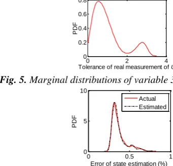
As discussed in Section 3.3, variable 3 (tolerance of real measurements of U) is the main concern in the study. In this subsection, variable 3 is further analysed. Copulas are applied to model the dependence structure between variable 3 and state estimation performance. The marginal distribution of variable 3 is given in Fig. 5, which is the probability density estimate of all potential combination of VTs and measurement classes listed in Section 3.2. Variable 3 is set to a set of values which are generated randomly based on the probability density given in Fig. 5, and the corresponding estimation errors are calculated and plotted by red solid line in Fig. 6. Copulas are used to model the dependence structure between the two series of data, v1 and

v2, which denote the observations of variable 3 and the

corresponding estimation errors respectively. Let u1 and u2

be the “probability integral transform” of v1 and v2

respectively, as introduced in Section 2.2, 𝒖 = [𝑢₁, 𝑢₂]’~𝑪. Thus, the scatterplot of u1 against u2, which is equivalent to

the copula, is shown in Fig. 7 to visualize the dependence structure. It can be seen that the scattered points are more tightly clustered around the diagonal in the upper tail (higher part of uncertainty range), indicating stronger dependence in joint events in upper tail than that in lower tail (lower part of uncertainty range).

Fig. 5. Marginal distributions of variable 3

Fig. 6.PDF of estimation errors

Fig. 7. Scatterplot of u1 against u2 for illustration of

dependence function

The nine copulas given in Section 2.2 are used to fit the two series of observations. Based on the ranking of log-likelihood among the nine copulas, the first four copulas as listed in Table 4 can adequately present the structural relationship between u1 and u2, while the others do not fit

the given data due to their poor log-likelihood results. It can be seen that among the copulas, the rotated Clayton’s copula has the best performance in modeling the dependence structure between u1 and u2, followed by SJC and Gumbel.

The rotated Clayton’s copula implies greater dependence for upper tail than for lower tail. The Gumbel’s copula implies the same. As for SJC, the estimated upper and lower tail dependence coefficients, 𝜏𝑈 and 𝜏𝐿, are 0.7817 and 2.9E-7 respectively; this also suggests low dependence in lower tail and high dependence in upper tail. For the purpose of comparison, the lower and upper tail dependence coefficients obtained by each copula are calculated and provided in Table 4 as well. It can be seen that the first three copulas present similar dependence structures with similar tail dependence coefficients, which are in line with the scatterplot in Fig. 7.

To demonstrate the appropriateness of using the estimated copula to represent the structural dependence of the observed data, bivariate data u1 and u2 are estimated

based on rotated Clayon’s copula together with its estimated copula parameter, i.e., the fittest copula provided in Table 4, using inverse CDF transformation. The probability density of the state estimation error obtained based on the estimated bivariate data is given by dash-dot line in Fig 6. It can be seen that the shape of the PDF obtained based on the estimated data is very similar to that of the actual data, i.e., the solid line in Fig 6, which demonstrates the accuracy of the copula estimated.

Table 4 Ranking of Estimated Copulas for Distribution in Fig. 5

Rank Copula index

Copula 𝐶𝜃 Tail dependence

Lower Upper

1 3 Rotated Clayton 2.7573 0 0.7777

2 9 SJC 0.7817 2.9E-7 2.9E-7 0.7817

3 6 Gumbel 2.4865 0 0.6785

4 4 Plackett 20.3437 0 0

Furthermore, the sensitivity of variable 3 is analysed at the upper tail and lower tail respectively by Morris screening method. The Morris ranking shows that variable 3 at upper tail (𝜇∗=0.21%) is more sensitive to variable 3 at the lower tail (𝜇∗=0.17%), as greater 𝜇∗ suggests higher sensitivity, as discussed in Section 2.2. To further demonstrate this, within lower tail, variable 3 is changed from 1.1% to 0.1% (improvement of 1%). This resulted in the improvement of state estimation performance by 25% with absolute improvement of 0.11%. On the other hand,

0 2 4

0 0.2 0.4 0.6 0.8

Tolerance of real measurement of U

P

D

F

0 0.5 1

0 5 10

Error of state estimation (%)

P

D

F

Actual Estimated

0 0.5 1

0 0.5 1

u

1

7 within upper tail, variable 3 is set from 3.0% to 2%

(improvement of 1% as well), resulting in estimation performance improvement by 30.8% with absolute improvement of 0.2%. It can be concluded therefore that the improvement of measurement tolerance at the upper tail results in greater improvement of state estimation performance. In this case, if the tolerance is located at the upper tail, the improvement of the measurement tolerance can be recommended due to the high dependence between the tolerance improvement and the improvement of state estimation. This analysis provides useful information for making decision on mitigation levels (i.e., how much uncertainty mitigation is needed) which might vary depending on the present location of the concerned variables within the possible range.

4. Conclusions

This paper presents the strategy/procedure that analyses and models the sensitivity and dependence structure of uncertain parameters in distribution system sate estimation. The sensitivity analysis technique of Morris screening method and copula theory are explored for this purpose and illustrated on a 295-bus realistic network model of a generic distribution system. The sensitivity of the critical variable in different zones is analysed and ranked in the study. It shows that the sensitivity level of the critical variable varies zonally. Due to the non-linear characteristic between the critical variable and SE performance, their dependence structure is analysed using copula theory with nine widely used copulas. It shows that whether the improvement of tolerance should take place is also depending on the dependence section the tolerance currently locates in.

The performed analysis provides useful information for planning monitoring reinforcement and developing efficient and effective mitigation strategies. Accurate assessment of the importance among different uncertainties and analysis of the dependence structure can guide power system operators towards variables that require the greatest mitigation or increased monitoring accuracy, and such assist them in making decisions about the location and accuracy of monitors for the purpose of state estimation.

5. Acknowledgments

This work was supported by H2020 Project NOBEL GRID under Grant 646184 and EPSRC UK through the ICUPS (Identifying Critical Uncertainties in Power Systems) project (EP/N004310/1).

6. References

[1] Abur A., Exposito A.G.: 'Power System State Estimation: Theory and Implementation' (Marcel Dekker, New York, 2004)

[2] Yih-Fang H., Werner S., Jing H., et al.: 'State estimation in electric power grids: meeting new challenges presented by the requirements of the future grid', IEEE Signal Proc. Mag., 2012, 29, (5), pp. 33-43

[3] Nanchian S., Majumdar A., and Pal B. C.: 'Three-phase state estimation using hybrid particle swarm optimization', IEEE Trans. Smart Grid, 2015, 8, (3), pp. 1035-1045

[4] Ke L.: 'State estimation for power distribution system and measurement impacts', IEEE Trans. Power Syst., 1996, 11, (2), pp. 911-916

[5] Minguez R., Conejo A. J.: 'State estimation sensitivity analysis', IEEE Trans. on Power Syst., 2007, 22, (3), pp. 1080-1091

[6] Macii D., Barchi G., and Petri D.: 'Uncertainty sensitivity analysis of WLS-based grid state estimators'. Proc. Int. Workshop on Applied Measure. for Power Syst., Aachen, Germany, Sep 2014, pp. 1-6

[7] King D.M., Perera B.J.C.: 'Morris method of sensitivity analysis applied to assess the importance of input variables on urban water supply yield – A case study', J. of Hydr., 2013, 477, pp. 17-32

[8] Hasan K., Preece R., Milanovic J.V.: 'Priority ranking of critical uncertainties affecting small-disturbance stability using sensitivity analysis techniques, (DOI 10.1109/TPWRS.2016.2618347)' IEEE Trans. on Power Syst. 2017, 32, (4), pp. 2629-2639

[9] Iooss B., Lemaıtre, P.: 'A Review on Global Sensitivity Analysis Methods', (Springer, 2015)

[10] Preece R., Milanovic J.V.: 'Assessing the applicability of uncertainty importance measures for power system studies', IEEE Trans. on Power Syst., 2015, 31, (3), pp. 2076-2084

[11] Patton A.J.: 'Copula-based models for financial time series," in Andersen T.G., Davis R.A., Kreiss J.P., Mikosch T. (Ed.) 'Handbook of Financial Time Series' (Springer Verlag, 2007)

[12] Bina M.T. Ahmadi D.: 'Stochastic modeling for the next day domestic demand response applications', IEEE Trans. on Power Syst., 2015, 30, (6), pp. 2880-2893

[13] Woolley N.C., Milanović J.V.: 'Statistical estimation of the source and level of voltage unbalance in distribution networks', IEEE Trans. Power Del., 2012, 27, pp. 1450-1460

[14] Morris M.D.: 'Factorial sampling plans for preliminary computational experiments', Technometrics, 1991, 33, (2), pp. 161-174

[15] Campolongo F., Cariboni J., Saltelli A.: 'An effective screening design for sensitivity analysis of large models', Environ. Modell. Soft., 2007, 22, (10), pp. 1509-1518

[16] Patton A.J.: 'On the out-of-sample importance of skewness and asymmetric dependence for asset allocation', J. of Finan. Econo., 2004, 2, (1), pp. 130-168

8 networks with renewable generation', IEEE Trans. on Power

Del., 2016, 32, (4), pp. 1975-1985

[18] Roytelman I., Shahidehpour S.M.: 'State estimation for electric power distribution systems in quasi real-time conditions', IEEE Trans. Power Del., 1993, 8, (4), pp. 2009-2015

[19] Alimardani A., Therrien F., Atanackovic D., et al.: 'Distribution system state estimation based on nonsynchronized smart meters', IEEE Trans Smart Grid, 2015, 6, (6), pp. 2919-2928

[20] IEC 61869-2:2012, 'Instrument transformers – Part 2: Additional requirements for current transformers' (2012)

[21] IEC 61000-4-30:2003, 'Testing and measurement techniques – Power quality measurement methods' (2003)

[22] Asprou M., Kyriakides E., Albu M., 'Bad data detection considering the accuracy of instrument transformers'. Proc. IEEE PES GM, Boston, U.S.A., 2016

[23] Singh R., Pal B.C., Vinter R.B., 'Measurement placement in distribution system state estimation', IEEE Trans. Power Syst., 2009, 24, (2), pp. 668-675

[24] HiPerDNO/2011/D.2.2.1, 'Report on Use of Distribution State Estimation Results for Distribution Network Automation Functions ' (2011)

[25] Hesmondhalgh S., 'GB energy demand-2010 and 2025. Initial brattle electricity demand-side model-scope for demand reduction and flexible response' (2012)

[26] EN 50160:2004, 'Voltage disturbances standard EN 50160 - voltage characteristics in public distribution systems' (2004)

[27] Muscas C., Pilo F., Pisano G., Sulis S.: 'Considering the uncertainty on the network parameters in the optimal planning of measurement systems for Distribution State Estimation', Proc. Instrum. Measure. Tech. Conf., Warsaw, Poland, 2007, pp. 1-6

[28] IEC 60076-1:2000, 'Power transformers - Part 1: general', (2000)