Predicting terrain contours using a feed forward neural network

Engineering Applications of Artificial Intelligence 16 (2003) 465–472

Predicting terrain contours using a feed-forward neural network

Stephen Erwin-Wright

, David Sanders

*, Sheng Chen

a_{Motiontouch Ltd., Weybridge, Surrey KT13 8LD, UK}

b_{Department of Mechanical and Management Engineering, University of Portsmouth, Anglesea Building, Anglessa Road, Portsmouth,} Hampshire PO1 3DI, UK

c_{Department of Electronics and Computer Science, University of Southampton, Southampton SO17 1BJ, UK}

Abstract

Wheeled or tracked vehicles cannot move easily over much of the land surface of the earth. This paper describes research work to create walking machines that are able to travel when the terrain makes wheeled or tracked vehicles ineffective. These legged walking vehicles must be able to negotiate unknown environments with little or no knowledge of the terrain. A predictive terrain contour mapping strategy is proposed that uses a feed-forward neural network trained using a back-propagation algorithm to predict contours based on leg positions and orientations. The strategy is tested using the abilities of a tele-operated eight-legged robot named ‘‘Robug IV’’. Predicted performance is an improvement on previous implementations and a summarised comparison of the results for the four terrains is provided.

r2003 Elsevier Ltd. All rights reserved.

1. Introduction

Legged robots can be better than traditional wheeled or tracked vehicles in rough and unstructured terrain (Chen et al., 1999). They can provide greater mobility and better isolation from the irregularities of the terrain, they can be faster and use less fuel and do less

environmental damage. Conventional wheeled or

tracked vehicles cannot access much of the land surface of the earth (approximately 50%).

Robug IV (White et al., 1999) is an example of a legged robot. It is a compact, powerful, general-purpose

teleoperated eight-legged robot that can walk (

Shim-Min Song and Waldron, 1988), transition between surfaces, traverse of a 0.305 m-deep pit, and perform

autonomous omni-directional climbing. Robug IV is

made of aluminium to minimise weight and can carry 50 m of umbilical with a 5 kg payload. Humans can

easily carry Robug IVas it only weighs 40 kg.

The electromagnetic design concept of the vehicle followed the same design rules and principles that were applied to previous legged robots created during the

research, for exampleRobug III. The vehicles are ‘spider

like’ with a central body and eight peripheral two-link

legs. Each leg onRobug IVis 0.7 m long and consists of

two links with four actuated points at the abductor, hip, knee and ankle. The body is 0.3, long by 0.45 m wide

and 0.4 m high, and is shown inFig. 1.

Orientation of joints in the robot leg are controlled using double-acting pneumatic cylinders. Pneumatic actuators were used because they are lighter and environmentally more rugged than geared electric motors. Force control could be provided by the use of pneumatic actuation. Several design structures were considered, and a kinematic chain like that of the PUMA 560 robot was selected, comprising a vertical first axis of rotation and two mutually parallel horizontal axes for the second and third joints.

Pneumatic cylinders are non-linear devices. Their behaviour varied with the operating temperature. Leaks are common in pneumatic systems and they are difficult to prevent completely. This caused problems during the testing of the abilities of the robot.

Loading on different joints in the robot legs varied widely, for example due to the load being carried by the robot during a walking gait sequence or simply due to the position of a leg.

2. Prediction of unknown terrain

The legs of the robot needed to be lifted at the end of an effective stroke, returned, and placed to begin a

*Corresponding author. Tel.: +44-2392-842565. E-mail address:[email protected] (D. Sanders).

support stroke. This created a phasing problem defined by the term ‘gait’. A Fuzzy-Logic Adaptive Gait

(FLAG) algorithm (Galt and Luk, 1997;Lehtokangas,

1999;Kendall et al., 1993) determined when to lift and when to place a leg. The FLAG algorithm was capable

of navigating Robug IV across terrains but problems

arose because the FLAG algorithm faithfully followed

the contours of obstacles. For example, whenRobug IV

detected a collision during a placement phase, a blind foothold search strategy was executed.

In the situation shown inFig. 2, the FLAG algorithm

deduced that the leg was in the vicinity of the lower kinematic workspace. The course of action to take was

to lift the leg higher in the z-axis. To execute this

process, a small force was exerted in the direction of the

detected obstacle during lifting the foot in order to feel

for the top surface of the obstacle.

As can be seen inFig. 2, after rejecting placement B,

Robug IV moved the leg and foot a number of times before it placed its foot at C. A terrain mapping system

that could predict unknown terrain could improve such a move by preventing a ‘juddery’ action during the move from A to C. The system could assist the smooth and efficient walking motions of legged robots in unstructed environments. This is could be important when accuracy of vision-based systems may be reduced in poorly lit or smoke filled environments. In the local area, a predica-tion system may provide more accurate informapredica-tion than a vision system. The better the predictive strategy,

the smoother Robug IV’s path, free of turnings and

vibrations.

Robug IV already had a terrain mapping system

capable of predicting thez-axis of the terrain (Warwick

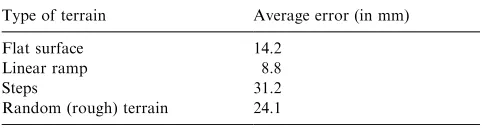
et al., 1995). The network used for this was trained for 5000 epochs to predict the next step, based on data from 5 previous steps. The average prediction errors for four

real terrain surfaces are shown inTable 1.

The sensors used in the robot had an error after

calibration of 76 mm so the artificial neural network

(ANN) needed to perform within this error. The

prediction errors shown inTable 1were large compared

to the sensor error.

They-axis was not predicted.

3. Improving the strategy using ANNs

Neural networks are useful for control and prediction

problems (Firschein and Fischler, 1987; Sanders et al.,

1994, 1996). Their ability to capture and model information from non-linear systems and generalise information from learned data makes them suitable for terrain prediction.

Under certain conditions it may be possible to extend the suitability theories that exist in traditional control theory to systems that include neural networks. This is important if an intelligent control structure for a walking machine is going to be adopted. The proposed new solution used a feed-forward neural network

(FFNN), trained using a back-propagation (Jones,

1995) supervised training algorithm. Variables predicted

for each leg are shown inFig. 4ofUrwin-Wright et al.

(2002). The layout ofRobug IVis shown here inFig. 3. IfRobug IVwere traversing forward in a straight line

from right to left as shown in Fig. 2, then it could be

assumed that the odd legs (1,3,5 and 7) would encounter

Fig. 2. Moving a foot from A to C. Fig. 1. Robug IV.

Table 1

Average prediction error for different types of terrain

Type of terrain Average error (in mm)

Flat surface 14.2

Linear ramp 8.8

Steps 31.2

the same terrains as their opposite legs (0, 2, 4 and 6) within 0.45–1.85 m (noting that the leg length is 0.7

(2) and width is 0.45).

The new neural network would benefit from having some of these inputs fed into it. Therefore, prediction might only be required for the leading legs.

The FLAG algorithm for Robug IV stated that at

least three legs must support the robot before a leg could be lifted and placed. When there were fewer than

two legs on either side,Robug IVwent into a lockdown

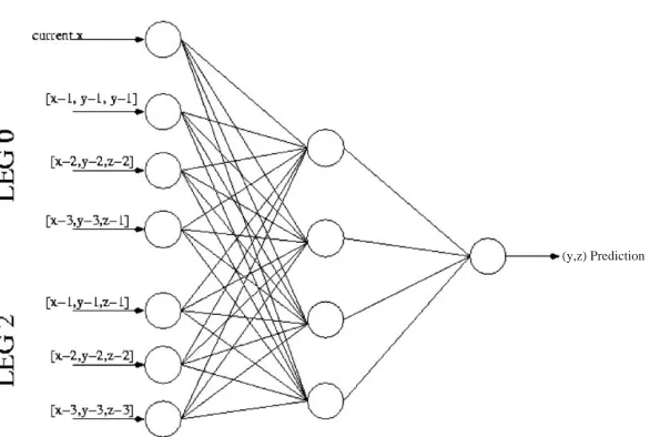
state to prevent damage. Assuming the robot was moving then the number of legs on each side of the body could vary from two to four. If the network was designed such that all four legs provided inputs to it but two of these legs might be redundant then what should these inputs be? An example solution is shown in Fig. 4.

Each leg onRobug IVhad four Siemens C167

micro-controllers. These micro-processors limited the memory available, so the design had to be compact compared to the power of the desktop PC used for simulation. This constraint needed to be considered when designing the network.

4. Testing the new strategy

A simulation called RobSim existed that consisted of an environment with a robot walking in it. The simulation had been used to test the FLAG algorithm

that was already incorporated intoRobug IV. This code

had been proved to emulateRobug(Urwin-Wright et al.,

2002) so it was decided to use the virtual environment

and the models to simulate the operation ofRobug IV.

Past experience had shown that simulation could some-times suggest that robots and systems can work when they later prove to be unable to cope in practice (Brooks, 1991). Although simulation can sometimes confuse the issue during engineering design, simulation

was selected for the initial trials and tests becauseRobug

IV was an expensive piece of equipment, capable of

damaging itself. Simulation provided a cost effective, safe and east way to test different gait strategies and especially to reject ideas and algorithms that did not work.

There was also a lack of random workspace to test all

the adaptive gait strategies asRobug IVneeded to walk

for considerable distances over a variety of terrains. The

only real way to test Robug IV’s step-climbing ability

was take a set of steps and let it traverse them. Problems arose with permission to conduct tests and with moving

equipment, air supplies andRobug IV to test sites. The

initial work was completed with simulations and a

virtualRobug IV and then selected terrains were tested

withRobug IVto confirm results.

Initial simulations were conducted without accelera-tion, which simplified things. The environment consisted of a surface that the robot walked over. The robot needed to be able to find out if a given point in space was above or below the surface, for example whether it

(y,z) Prediction

Fig. 4. ANN arrangement to provide a prediction inyandz:

had made contact. The simplest way to model the various surfaces was as a series of planar tiles.

Training and testing were similar as the training sequence was close to the testing sequence and both came from the same source. Using RobSim, data was acquired for a range of terrains. As RobSim had been proved, the mathematical calculations remained the

same. The x-step that was originally used was 0.26 m

(Galt and Luk, 1997); therefore one step was roughly 0.26 m. This data was then formulated into previous step, next step, training and testing data.

Testing routes were 4000 m long to provide sets of samples, that was roughly 15,000 steps. From this, the training and testing were derived. These sets were then

applied to a genetic FFNN (Goldberg, 1988;Luk et al.,

2000). The number of inputs was then varied along with

the numbers of hidden neurons in order to find the optimum configuration; within the constraints men-tioned earlier in Section 3. Rules developed for one leg inFig. 3were applied to the other legs. As an example, the results for leg 0 are shown in the next section but the rules for leg zero were applied to the other seven; leg 0 was used for initial testing and then results were implemented on the other legs.

It was not possible forRobug IV to manoeuvre with

fewer than two legs per side. Robug IV went into a

lockdown state when this occurred. To overcome the problem of which legs to feed into the networks, the network was designed with only two legs for the inputs. So the previous steps from leg 2 constituted the other input to the network.

5. Results

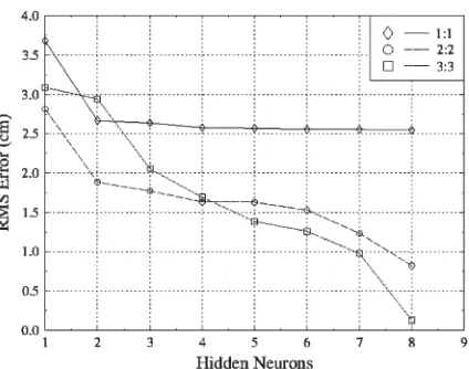
Testing took place over the routes to provide the sets of samples. These sets were then applied to the genetic FFNN. The number of inputs was varied along with the numbers of hidden neurons in order to find the optimum configuration. The optimum number of input and hidden layers neurons was defined as the point when no more advantage was identified in increasing their number during the testing phase. The first value to be set

was the number of input neurons.Galt and Luk (1997)

and Urwin-Wright et al. (2002)stated that the number of hidden layers should be four, trained for 5000 epochs. The number of previous steps that were being fed back into the network ranged from one to three. Above three, the size of the FFNN became unworkable within the constraints of the robot systems; below one, the FFNN

became inane. The RMS prediction of they-andx-axis

plotted against the number of hidden neurons is shown in Figs. 5 and 6.

From the RMS prediction error of they-axis shown in

Fig. 5, all the previous steps fed into the network appear in ascending order. Using more than two hidden

neurons significantly reduced the error of the prediction, and using more than eight reduced the RMS of the prediction to less than 1.0 cm.

The RMS prediction of thez-axis shown in Fig. 6 is

interesting. Feeding three previous steps into the network and having less than four hidden neurons resulted in the network performing worse than when two previous steps are fed into the network. As with only using two previous steps, having more than eight hidden neurons reduced the RMS error to below 1.0 cm and even close to 0.25 cm.

Considering the error of the pneumatic cylinder once

it had been calibrated, which was76 mm; to reduce the

RMS error to within this amount would require at least eight hidden neurons and three previous steps to be fed into the network. Problems arose here, as achieving this result increased the demand on the micro-controllers. It was decided than an RMS error of 1.6 cm was tolerable; taking advantage of the fact that when using two previous steps the network performance was better. So two previous steps were fed were into the FFNN, with four hidden neurons. The following results show now

Fig. 5. y-Axis RMS error over all terrains.

the network performed over the four terrains listed in Table 1.

The figures illustrating these results use error in cm rather than error squared. Because the error is small, squaring made the graphics appear as straight lines in the paper.

5.1. Predicting the y-axis

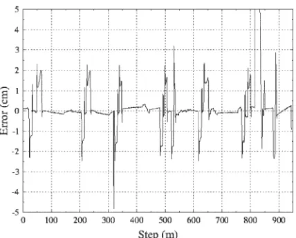
Fig. 7shows the position of the leg in they-axis when

Robug IV was walking up a ramp. The error in the

prediction of this ramp is shown in cm in Fig. 8; the

RMS error of this is 0.450374 cm.

Fig. 9shows the position of the leg in they-axis when

Robug IVwas walking across rough terrain. The error in

the prediction of this terrain is shown in cm inFig. 10;

the RMS error of this is 2.418234 cm.

Fig. 11 shows the position of the leg in the y-axis whenRobug IVwas walking across smooth terrain. The error in the prediction of this terrain is shown in cm in Fig. 12; the RMS error of this is 0.422875 cm.

Fig. 13 shows the position of the leg in the y-axis when Robug IV was walking up a set of stairs is

shown in cm in Fig. 14; the RMS error of this is

8.256384 cm.

Fig. 7. Ramp terrain.

Fig. 9. Rough terrain.

Fig. 10. Position error fory-axis over the rough terrain.

Fig. 11. Smooth terrain.

5.2. Predicting the z-axis

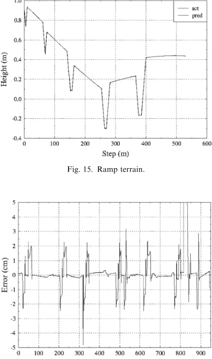
Fig. 15shows the position of the leg in thez-axis when

Robug IV was walking up a ramp. The error in the

prediction of this ramp is shown in cm inFig. 16; the

RMS error of this is 2.541913 cm.

Fig. 17shows the position of the leg in thez-axis when

Robug IVwas walking across rough terrain. The error in

Fig. 12. Position error fory-axis over the smooth terrain.

Fig. 13. Stair terrain.

Fig. 14. Position error fory-axis over the stair terrain.

Fig. 15. Ramp terrain.

Fig. 16. Position error forz-axis over the ramp terrain.

the prediction of this terrain is shown in cm inFig. 18. The RMS error of this is 2.541913 cm.

Fig. 19shows the position of the leg in thez-axis when

Robug IVwas walking across smooth terrain. The error

in the prediction of this terrain is shown in cm inFig. 20;

the RMS error of this is 0.352966 cm.

Fig. 21shows the position of the leg in thez-axis when

Robug IVwas walking up a flight of stairs. The error in

the prediction of these stairs is shown in cm inFig. 22;

the RMS error of this is 2.541913 cm.

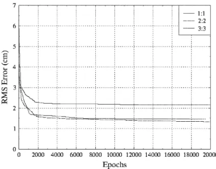
5.2.1. Learning rate (epochs)

The two best predictions were obtained with four and eight hidden neurons. The learning rate of the three

different inputs is shown inFigs. 23 and 24.

Fig. 23 suggests that there is no significant

advantage in network learning with more than 2000 epochs, as the RMS prediction error does not improve much.

With eight hidden neurons the network learning levels

off at around 2600 epochs as shown inFig. 24. As only

four hidden neurons were used, the optimum epoch training sequence had only 2000 epochs.

Fig. 18. Position error forz-axis over the rough terrain.

Fig. 19. Smooth terrain.

Fig. 20. Position error forz-axis over the ramp terrain.

Fig. 21. Stair terrain.

6. Conclusion

The terrain prediction did not predict the y-axis

location of the robot legs, so there is no comparison for

the y-axis prediction; a summary of results is given in

Table 2.

A summary of the results for the z-axis prediction

comparisons for four terrains is shown inTable 3.

Assuming that the terrains tested in the old imple-mentation are similar to those tested with new FFNN, then the new network performed better than the old network on rough, smooth and stair surfaces. The

results for the ramp terrain shown in Fig. 15 are not

completely linear, and this may account for the poorer

result in the z-axis. It was also assumed that ‘average

error’ quoted in the previous result was actually the RMS error. The number of epochs is significantly smaller. The old implementation used 5000 epochs; the new implementation uses less than half that, at 2000 epochs. This reduced implementation time.

References

Brooks, R., 1991. Intelligence without reason. MIT AI Lab memo 1(1293)http://www.leglab.ai.nit.edu.

Chen, S., Istepanian, R., Gait, S., Luk, B., 1999. Intelligent Walking Gait Generation for Legged Robots. Professional Engineering Publishing, Bury St. Edmunds, UK.

Firschein, O., Fischler, M., 1987. The Eye, The Brain and The Computer. Addison-Wesley, UK and USA.

Galt, S., Luk, B., 1997. Predictive terrain contour mapping for a legged robot. Fifth International Conference on Artificial Neural Networks, University of Reading, UK, pp. 129–133.

Goldberg, D.E., 1988. Genetic Algorithms in Search, Optimisation and Machine Learning. Addison-Wesley, Reading, MA.

Jones, A., 1995. Neural networks and genetic algorithms for prediction and control of dynamic systems. Technical Report, Imperial College, London.

Kendall, W.S., Barndorff-Nielsonm, O.E., Jensen, J.L., 1993. Networks and Chaos—Statistical and Probabilistic Aspects. Chap-man & Hall, London.

Lehtokangas, T.M., 1999. Additive neural networks and periodic patterns. Neural Networks 12 (4–5), 617–626.

Luk, B.L., Gait, S., Chen, S., 2001. Using genetic algorithms to establish efficient walking gaits for an eight-legged robot. Interna-tional Journal of Systems Science 32 (6), 703–713.

Sanders, D.A., Haynes, B.P., Vogt, M., Stott, I.J., 1994. Control of a robot using neural networks as feed forward estimators and as feedback controllers. Proceedings of European Robotics and Intelligent Systems Conference, Vol. (B), Spain, pp. 1065–1074. Sanders, D.A., Haynes, B.P., Tewkesbury, G.E., Stott, I.J., 1996. The

addition of neural networks to the inner feedback path in order to improve on the use of pre-trained feed forward estimators. Journal of Mathematics and Computers in Simulation 41, 461–472. Song, S.-M., Waldron, K., 1988. Machines that Walk: the adaptive

suspension vehicle. MIT Press, Cambridge, MA.

Urwin-Wright, S., Chen, A., Sanders, D.A., 2002. Terrain prediction for an eight-legged robot. Journal of Robotic Systems 19 (2), 91–98.

Warwick, K., Irwin, G., Hunt, K., 1995. Neural Network Applications in Control, IEEE Control Engineering Series, Vol. 53. Academic Press, Exeter, England.

White, T., Luk, B., Cooke, D.S., Hewer, N., 1999. Implementation of Modularity in Robug IV—Preliminary Results. Professional Engineering Publishing, Bury St. Edmunds, UK.

Fig. 24. Network learning with eight hidden neurons.

Table 2

y-Axis error for different types of terrain

Type of terrain RMS prediction error in cm

Stair 8.2564 Smooth 0.4229 Rough 2.4182 Ramp 0.4504 Collective 2.887 Table 3

Comparisons ofz-axis error for different types of terrain

Type of terrain

RMS error of new prediction in cm

Average error of old prediction in cm

Stair 2.1348 3.12

Smooth 0.353 1.42

Rough 1.4984 2.41

Ramp 2.5418 0.88

Collective 1.6321 1.96