J. Phys. A: Math. Gen.36(2003) 6611–6628 PII: S0305-4470(03)59450-1
Correlations and screening of topological charges in
Gaussian random fields
M R Dennis
H H Wills Physics Laboratory, Tyndall Avenue, Bristol BS8 1TL, UK
Received 10 February 2003, in final form 24 April 2003 Published 5 June 2003
Online atstacks.iop.org/JPhysA/36/6611
Abstract
Two-point topological charge correlation functions of several types of geometric singularity in Gaussian random fields are calculated explicitly, using a general scheme: zeros ofn-dimensional random vectors, signed by the sign of their Jacobian determinant; critical points (gradient zeros) of real scalars in two dimensions signed by the Hessian; and umbilic points of real scalars in two dimensions, signed by their index. The functions in each case depend on the underlying spatial correlation function of the field. These topological charge correlation functions are found to obey the first Stillinger-Lovett sum rule for ionic fluids.
PACS numbers: 02.40.Hw, 02.50.−r, 05.20.Jj
1. Introduction
Although a spatially extended field may be smooth, and contain no infinities, it may nonetheless have point singularities associated with its topology. For example, a two-dimensional landscape, specified by a real function, hascritical points(stationary points), where the gradient of the field vanishes and the gradient direction cannot be defined; in the neighbourhood of such a point, the gradient direction changes arbitrarily quickly through all of its values. Such points are characterized by atopological charge, a signed integer which is determined by the local geometry of the singularity; in the case of critical points, the number is the (signed) number of rotations of the gradient vector around the critical point; it is +1 for maxima and minima, and−1 for saddles. The topological charge is also called thePoincar´e index(orHopf index) (Milnor 1965), and is defined as a signed integer at the point zeros ofn-dimensional real vector fields inndimensions. Although the number of zeros may change as a field evolves, the total topological charge is constant; it is a topological invariant.
Here, I discuss the statistical properties of various zeros/singularities, in fields which are specified by Gaussian random functions. In this case, only structurally stable zeros of charge±1 occur. Specifically, I shall discuss how densities and two-point charge correlation functions of the distributions of signed singularities may be calculated under a rather general
scheme, and then use this scheme to calculate the topological charge correlation functions of three types of singularity in isotropic random fields: zeros of n-dimensional vectors in
n-dimensional space (rederiving a result originally due to Halperin (1981)); critical points of random scalar fields in two dimensions; and umbilic points of random scalar fields in two dimensions. The charge correlation functions for each of these types of topological singularity are found to be different in each case, and dependent on the underlying correlation function of the Gaussian field. Each function is found to satisfy a screening relation associated with ionic liquids.
Topological zeros are very important in many areas of physics and mathematics: in addition to critical points (gradient zeros) which have obvious importance, the zeros of two-dimensional complex scalar fields (phase singularities, wave dislocations, vortices, realised as two-dimensional vectors) are also of great interest, especially where the field is a quantum wavefunction or an optical field (e.g., Nye and Berry (1974), Berry and Dennis (2000), Dennis (2001b)), or an order parameter (Mermin 1979). Only point zeros are considered here—the dimensionalitynof the vector field, whose zeros provide the singularity, is assumed equal to the dimensionality of the space.
The first systematic study of the statistical geometry of random real scalar fields in two dimensions was by Longuet-Higgins (1957a,1957b, 1958), who generalized one-dimensional methods of Rice (1954) to calculate, amongst other things, the densities of critical points and probability density function of the Gaussian curvature of the function. Halperin (1981) derived then-dimensional vector correlation function, whose proof was supplied by Liu and Mazenko (1992), and has recently been recast in the language of Riemannian geometry by Foltin (2003a). Various correlation functions in two dimensions, including those for phase singularities and critical points, were investigated numerically by Freund and Wilkinson (1998). Planar phase singularity correlations (including density correlations) were investigated by Berry and Dennis (2000).
The topological singularities of interest are the zeros of ann-dimensional vector field v=(v1, . . . , vn).The field is a smooth function defined on ann-dimensional Euclidean space, with points labelled by the vectorr = (r1, . . . , rn).In random fields, the only statistically
significant zeros are those of first order, whose Jacobian determinant
J =det∂ivj (1.1)
is nonzero (where∂i ≡ •,i ≡∂/∂ri). The topological charge of such zeros is given by signJ.
When the field is random, the densityd(r)of zeros at a positionris
d(r)= δn(v(r))|J(v(r))| (1.2)
where• denotes averaging over the statistical ensemble, and the zeros are identified by then-dimensional Diracδ-function. The modulus of the Jacobian is included to ensure that each zero has the correct statistical weight, sod(r)has the units of density. This expression confirms that degenerate zeros are so rare they have no statistical significance. The average topological chargeq(r)atris expressed as the density (1.2), but each singularity is weighted by its charge, that is, the sign of the Jacobian. The charge correlation functionsgwith which this paper is concerned are the generalization of the average charge density to that at two pointsrA,rB,normalized by the density:
g(rA,rB)=
1
d(rA)d(rB)
δn(v(rA))δn(v(rB))J(v(rA))J(v(rB)). (1.3)
is then applied to zeros of n-dimensional vector fields (section4), critical points of two-dimensional scalar fields (section5), and umbilic points of the same fields (section6). The phenomenon of topological charge screening in these three cases is discussed in section7.
As this paper was being completed, I became aware of the work of Foltin (2003b), who performs similar calculations for critical points by a different, possibly simpler method.
2. Gaussian random functions and scheme for calculating charge correlation functions
An ensemble of scalar functionsf inn-dimensional space is said to be aGaussian random functionif the probability distribution of the function at each point of space is given by a Gaussian distribution, so the function at each point defines a Gaussian random variable (Adler 1981). The only restrictions on Gaussian random functions made in this section are that they be centred (the averagef =0) and that first derivatives exist.
Our starting point is the well-known expression for the probability density function for a set ofNindependent Gaussian random functionsu=(u1, . . . , uN),
P (u)= exp(−u·Σ
−1·u/2)
(2π )N /2√detΣ (2.1)
whereΣis thecorrelation matrix, with components defined
ij = uiuj. (2.2)
It is now possible to present the general scheme for calculating 2-point topological charge correlation functions of zeros of Gaussian random functions, expressed in (1.3). The topological charges considered are all zeros of a real vector Gaussian random function v=(v1, . . . , vn),of dimensionn,and the correlation function is the average of the product
of the local density at points labelledA, B.Quantities evaluated at these places are denoted with the appropriate subscriptA or B. The variables that appear in the average (1.3) are therefore the components ofvA,vB,and their derivatives∂vA, ∂vBthat appear in the Jacobians
J(vA)≡JA,J(vB)≡JB.There are a total ofmdifferent derivatives∂ivjappearing in each
Jacobian, and in generalmn2.For example, in the case of critical points,n=2, andm=3 (the terms appearing in the Jacobian are∂11f, ∂22f, ∂12f =∂21f). The calculation therefore involves an average of theN =2(m+n)-dimensional Gaussian random vector
u=((∂vA)1, . . . , (∂vA)m, (∂vB)1, . . . , (∂vB)m, vA1, . . . , vAn, vB1, . . . , vBn). (2.3) The correlation matrixΣfor thisuis defined as in (2.2), and averages are evaluated according to the probability density function (2.1).
The correlation function in (1.3) is therefore,
gAB=
δn(vA)δn(vB)J AJB d(rA)d(rB)
= 1
d(rA)d(rB)(2π )n+m√detΣ ×
d2(n+m)uδn(vA)δn(vB)JAJBexp(−u·Σ−1·u/2) (2.4)
whered(rA), d(rB)are the appropriate densities of zeros (1.2). The JacobiansJA,JB can
be quite complicated; each is a multilinear function, involving a sum ofn-fold products of
u1, . . . , um(forA) orum+1, . . . , u2m(forB).
The 2n×2n-dimensional lower right submatrix ofΣ(i.e., the averages dependent only onvA,vB) is denoted byK;the complementary 2m×2m-dimensional upper left submatrix
ofΣ−1is denoted byΞ−1;that is,
Σ=
• •
• K
Σ−1 =
Ξ−1 •
• •
where the other blocks marked•are not denoted by special symbols. In appendix A, Jacobi’s determinant theorem is used to show that
detΣ=detKdetΞ. (2.6)
The integrals invA1, . . . , vBn,only involvingδ-functions, are performed, leaving the 2m derivative terms∂vto integrate; letu=((∂vA)1, . . . , (∂vB)m).Then
gAB= 1
d(rA)d(rB)(2π )n+m √
detΣ
d2muJ
AJBexp(−u·Ξ−1·u/2)
= 1
d(rA)d(rB)(2π )n+m √
detΣ
d2muJAJB √
detΞ
(2π )m
d2mtexp(it·u−t·Ξ·t/2)
(2.7)
upon Fourier transforming the Gaussian in u with the 2m-dimensional Fourier vector variable t. The Jacobian terms JA (depending on u1, . . . , um) and JB (depending on um+1, . . . , u2m) may be replaced with partial derivative terms intj,
uj →i∇tj =i∇j (2.8)
where∇is used to denote partial derivatives in 2m-dimensionalt-space. The Jacobians, with this replacement, have now become differential operators, denotedJ∇A,J∇B.Therefore,
gAB= 1
d(rA)d(rB)(2π )n+2m
detΞ
detΣ
d2mtexp(−t·Ξ·t/2)J
∇AJ∇B
d2muexp(it·u)
= 1
d(rA)d(rB)(2π )n+2m (2π )2m √
detK
d2mtexp(−t·Ξ·t/2)J∇AJ∇Bδ2m(t) (2.9)
where, in the second line, the integral overu is realized as the Fourier transform of the
δ-function oft,and (2.6) has been used in the prefactor. The expression is then integrated by parts (so theJ∇ operators act on the exponential term rather than theδ-function), and then integrated int.The final expression is
gAB = 1
d(rA)d(rB)(2π )n
1
√
detKD (2.10)
where
D=[J∇AJ∇Bexp(−t·Ξ·t/2)]t=0. (2.11)
The charge correlation function therefore only depends on d,detKand components of the inverse reduced inverse correlation matrixΞ.
This final step, evaluatingDin (2.11) is the most complicated part of the calculation, and depends on the precise form of the Jacobian determinantJ.Each summand in the operator J∇AJ∇Bis a 2n-fold derivative over some index set{τ} = {τ1, . . . , τ2n},and is comprised of
nterms from∇1, . . . ,∇m(forA), andnterms from∇m+1, . . . ,∇2m(forB), either set possibly
including repetitions. The result of this particular operation is
2n
j=1 i∇τj
exp(−t·Ξ·t/2)
t=0 =
all pairings
p (τλ,τλ)∈p
τλτλ (2.12)
where the sum on the right-hand side is over all pairingsp=(τα, τα)· · ·(τµ, τµ)of indices in
themselves are found by further application of Jacobi’s determinant theorem in appendix A, and are expressed in terms of minors of detΣin (A.3).
The correlation functions calculated explicitly in this paper are not too complicated, either becausenis small (only two-dimensional fields are considered in sections5,6), orΞis sparse, as in the case of random vectors (section4).
The densitydof zeros appears in (2.10); in general, this may be difficult to calculate, due to the modulus sign in (1.2). For randomn-dimensional vector fields, the main part of the density calculation is in appendix B. For critical and umbilic points, these densities were calculated by Longuet-Higgins (1957a, 1957b) and Berry and Hannay (1977).
3. Isotropic random fields
The topological charge correlation function in (2.10) is extremely general, applying to any centred differentiable Gaussian random vector field. In this section, and for the remainder of the article, attention will be restricted to stationary isotropic random fields. For these fields, all averages are (statistically) translation and rotation invariant. They are conveniently given by a Fourier representation
f (r)=
k
a(k)cos(k·r+φk) (3.1)
wherekare now the Fourier variable vectors (wavevectors). The componentsvi of random vectors are specified by independent identically distributed realizations of (3.1). The amplitude
a(k)only depends on the magnitude|k| =k,and the phaseφkis uniformly random—each ensemble member is therefore labelled by the choice ofφkfor eachk.It may also represent the spatial part of a real linear homogeneous nondispersive wavefield, for which the representation (3.1) is particularly evocative. The infinitekset is assumed sufficiently dense that they may be represented as an integral, and
k
a2(k)• ≈
dnk(k)• (3.2)
where(k) is the power spectrum of the field; by the Wiener-Khinchine theorem (Feller 1950),(k) is then-dimensional Fourier transform of thefield correlation functionC(r),
wherer= |rA−rB|,and
C(r)= fAfB = f (rA)f (rB) (3.3) normalized such thatC(0)= f2 =1.The only condition onCis that it is symmetric and has positive Fourier transform.
Averages of derivatives of f may be represented as moments of (as by Longuet-Higgins (1957a,1957b), Berry and Hannay (1977), Berry and Dennis (2000)), or equivalently derivatives ofCas is done here. Coordinates are chosen where
r=rB−rA r1=r rj =0 j =2, . . . , n. (3.4)
Since the fields are isotropic, the results are not affected by this choice. The correlations computed in sections5,6are in two dimensions; in this case, direction 1 is denoted by x,
direction 2 byy.
Representing derivatives by subscripts, the correlations of first derivatives off are found to be (Berry and Dennis 2000)
E≡ fA,1fB = −fAfB,1 = −[∂1C]r1=r,r2,...=0= −C
F ≡ fA,1fB,1 = −fA,11fB = −fAfB,11 = −
∂12Cr
1=r,r2,...=0= −C
(3.5)
H ≡ fA,jfB,j = −fA,jjfB = −fAfB,jj = −∂22Cr
1=r,r2,...=0= −C
Averages involvingf and its first derivatives other than those in (3.3), (3.5) are zero. The averages are equal to appropriate derivatives ofC(r),and then settingr1 = r, r2, . . .= 0 (as in (3.4)), and derivatives inrj of odd order vanish. The functions in (3.5), whenr=0 (denoted by subscript 0), are
E0 =0 F0=H0= −C(0)= −C0. (3.6)
It is easily verified that−C0>0,sinceChas a positive Fourier transform. The correlation matrices (5.4), (6.5) required to calculate the topological charge correlation functions of critical points and umbilic points, involve higher derivatives ofC,given in (5.5), (6.6).
As the separation betweenAandBincreases, the correlation betweenfAandfBdecreases and C → 0. This decay is slowest in the case where all the k in (3.1) have the same lengthk0, (set to 1 for convenience) and the power spectrum(k) = δ(k−1).For any
n > 2,the corresponding correlation function is a Bessel function times a factor ofr,with oscillatory decay that falls off liker−(n−1)/2. Of particular interest is the n = 2 case, for whichC(r) = J0(r).The spectrum in this case was called the ring spectrum by Longuet-Higgins (1957a,1957b) and Berry and Dennis (2000), and is conjectured to model the high eigenfunctions in quantum chaotic billiards (Berry 1978, 2002).
4. Correlations of zeros of isotropic vector fields
In the present section, we shall consider n-dimensional Gaussian random vector fields v=(v1, . . . , vn)inndimensions whose Cartesian components are independent and identically
distributed Gaussian random fields (the derivatives of the components are also assumed completely independent). The JacobianJ,whose sign determines the topological charges of the zeros, is the determinant of the matrix of first derivatives (1.1).
We begin by calculating the density (1.2) of zeros of random vectors. This was calculated for n = 1,2,3 by Halperin (1981) and Liu and Mazenko (1992), (the n = 1 case was previously found by Rice (1954), andn=2 by Berry (1978)). For generaln,the densitydn
(1.2) is expressed as a probability integral with density function (2.1) and correlations given by (3.5), (3.6). Therefore,
dn= δn(vi)|detvi,j|
= 1
(2π )n(n+1)/2Fn2/2 0
dnvidn2vi,jδn(v)|detvi,j|exp
−1
2
n
i=1
vi2−1
2
n
i,j=1
vi,j2
= F
n/2 0
(2π )n(n+1)/2
dn2vi,j|detvi,j|exp
−1
2
n
i,j=1
vi,j2
(4.1)
where in the final line theδ-functions in thevi were integrated, and thevi,j were rescaled (each by√F0) to be dimensionless. The remaining integral is solved in appendix B, giving the density of zeros inndimensions
dn=(−C0)n/2 n−1
2
!
π(n+1)/2 =(−C 0)
n/2(n−1)!σn−1
(2π )n . (4.2)
In this expression,σn−1is the surface area of the unit(n−1)-sphere inndimensions, given by (B.4). As is common in such problems in statistical geometry, the result is a spectral quantity
((−C0)n/2)multiplied by a geometric factor.
of the scheme is facilitated by the fact that the componentsviare completely independent, and m=n2.The submatrixK
nof the correlation matrixΣnonly depends on the correlations of
the components of the vectorsvA,vB;from section3, the only correlations that do not vanish arev2
Ai
=v2
Bi
=1 andvAivBi =Cfori=1, . . . , n.It is easy to see that
detKn=(1−C2)n. (4.3)
From (2.12), the other necessary ingredient of the correlation function scheme is the components of the matrixΞ,defined in (2.5). The elements ofΞare labelled by the multiindex of the components vAi,j, vBk,l; using the correlations (3.5), (3.6) and the arguments of appendix A, particularly equation (A.3), the only nonvanishing elements are
(Ai,1)(Ai,1)=(Bi,1)(Bi,1)=F0−E2/(1−C2)
(Ai,1)(Bi,1)=(Bi,1)(Ai,1)=F0−E2/(1−C2)
(4.4)
(Ai,j )(Ai,j )=(Bi,j )(Bi,j )=F0
(Ai,j )(Bi,j )=(Bi,j )(Ai,j )=H fori=1, . . . , n j =2, . . . , n.
The problem remains to use these components and (2.12) to evaluate (2.11). By (1.1), (2.8),
J∇A=det∇Ai,j (4.5)
(similarly for J∇B). Each of the n! summands in this determinant is an n-fold product
signσi∇Ai,σ (i),whereσ is a permutation of 1, . . . , n.Therefore,
J∇AJ∇B=
permutations
σ,σ
signσsignσ(−1)n n
i,j=1
∇Ai,σ (i)∇Bj,σ (i). (4.6)
From (2.12), the result of one of these summands acting on exp(−t·Ξ·t/2)and settingt=0 is nonzero if there is a pairing of these multiindices where the corresponding elements ofΞ
are nonzero. From (4.4), this is only the case when the permutationsσ, σare the same. Thus, from (2.12) and (4.4),
Dn=
permutations
σ n
i=1
(Ai,σ (i))(Bi,σ (i))
=n!
n
i=1
(Ai,i)(Bi,i)
=n!(F−CE2/(1−C2))Hn−1. (4.7)
This, together with (4.3), can now be put into (2.10) to give
gn(r)= n! 2π d2
n
(F (1−C2)−CE2)
(1−C2)3/2
H
2π√1−C2
n−1
= − n!
2π d2
n
(C(1−C2)+CC2)
(1−C2)3/2
−
C
2π r√1−C2
n−1
= (n−1)! (2π )nd2
nrn−1
dhn(r)
dr (4.8)
where the functionhn(r)is defined as
hn(r)=
−C √
1−C2
n
0.5 1 1.5 2 2.5 3 3.5
−1 −0.8 −0.6 −0.4 −0.2
(b)
2 4 6 8 10
−0.3 −0.2 −0.1 0.1
[image:8.595.99.469.87.199.2](a)
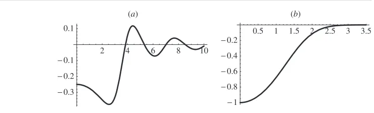
Figure 1.The two-dimensional vector zero correlation functiong2(r),plotted for two choices of
C(r): (a)C(r)=J0(r);(b)C(r)=exp(−r2/2).
This decays to 0 asr → ∞,and whenr=0,
hn(0)=(−C0)n/2 (4.10)
(the quantityC0=C(0)is always negative, sinceCis the Fourier transform of the positive power spectrum).
The topological charge correlation function of zeros ofn-dimensional Gaussian random vector fieldsg(r)was first calculated by Halperin (1981), in a form equivalent to (4.8), but without proof. This function was also derived by different means by Liu and Mazenko (1992), and in then=1 case by Rice (1954), and then =2 case by Berry and Dennis (2000) and Foltin (2003a). g(r) is plotted in figure1for two choices of the field correlation function
Cforn =2.WhenC(r) =J0(r), g2is oscillatory; whenC(r)=exp(−r2/2),it increases monotonically to zero asr→ ∞.
5. Critical points in two dimensions
In this section, the scheme of section2is used to calculate the topological charge correlation function of critical points of isotropic Gaussian random functions in the plane, that is the Poincar´e index correlation function of isotropic random surfaces.
The Gaussian random function examined shall be writtenf =f (r)=f (x, y)(where
x = r1, y = r2), which will be assumed stationary and isotropic, so the expressions in section3 may be used. In particular,f and its first derivatives have the correlations (3.5), (3.6), as well as further correlations involving second derivatives, described below. As in the previous section, for the convenience in calculations, the two pointsAandBare separated only in thexcoordinate.
At a critical point, the gradient∇f =(f,x, f,y)is zero. The critical point JacobianJc whose sign defines the topological charge (Poincar´e index) is the Hessian determinant
Jc=detf,ij =f,xxf,yy−f,xy2 (5.1)
this is the Gaussian curvature of the surface. Unlike a general two-dimensional random vector field (as in the previous section), the gradient field ∇f is irrotational, which gives rise to relationships and correlations between the derivatives of the components (e.g.,f,xy =f,yx,
The statistical properties of critical points of Gaussian random fields in two dimensions were considered by Longuet-Higgins (1957a,1957b); he found that the densitydcof critical points is (Longuet-Higgins 1957b, equations (71), (78)):
dc=
2C0(4)
3π√3C0
(5.2)
(C0(4)denotes the fourth derivative ofC,evaluated atr =0). The density of saddles equals the density of extrema (maxima and minima), and the density of maxima equals the density of minima. The probability density function of the Gaussian curvatureJ, despite its asymmetry (Longuet-Higgins 1958, equation (7.14); Dennis 2002, equation (57)), has zero first moment, implying the average topological chargeδ2(∇f )J
cis zero, as expected.
The topological charge correlation function is again calculated using the scheme of section2, particularly (2.10). Therefore, the vectoru(2.3) of Gaussian random variables, in a convenient ordering, is
uc=(fA,xx, fA,yy, fB,xx, fB,yy, fA,xy, fB,xy, fA,x, fB,x, fA,y, fB,y) (5.3)
with correlation matrix (cf (2.2))
Σc=
M0 L0 M L 0 0 0 G 0 0
L0 M0 L N 0 0 0 I 0 0
M L M0 L0 0 0 −G 0 0 0
L N L0 M0 0 0 −I 0 0 0
0 0 0 0 L0 L 0 0 0 I
0 0 0 0 L L0 0 0 −I 0
0 0 −G −I 0 0 F0 F 0 0
G I 0 0 0 0 F F0 0 0
0 0 0 0 0 −I 0 0 F0 H
0 0 0 0 I 0 0 0 H F0
(5.4)
where the correlations between elements ofucare computed to be
G≡∂x3Cx=r,y=
0=C
(3)
I ≡∂x2∂yC
x=r,y=0=(rC−C)/r 2
L≡∂x2∂y2Cx=r,y=0=(r2C(3)−2rC+ 2C)/r3
(5.5)
M≡∂x4Cx=r,y=
0 =C
(4)
N≡∂y4Cx=r,y=
0 =3(rC−C)/r 3
G0=I0=0 M0=N0=3L0=C0(4).
The last line gives the special value of these correlations whenr=0.
The matrixKcis the 4×4 lower right submatrix ofΣc,and has determinant detKc=
F02−H2F02−F2. (5.6)
The pair of differential Jacobian operators are, from (5.1),
J∇AJ∇B= ∇1∇2∇3∇4+∇52∇62− ∇1∇2∇62− ∇3∇4∇52. (5.7) Using (2.12), the result of these operators acting is on exp(−t·Ξ·t/2)and settingt=0 (cf (2.10), (2.11)) is
Dc=1423+1324−21626+1234− 23545−3455+ 2256
(b) (a)
2 4 6 8 10
−1.25 −1 −0.75 −0.5 −0.25 0.25
0.5 1 1.5 2 2.5 3 3.5
[image:10.595.109.469.86.199.2]−0.4 −0.3 −0.2 −0.1
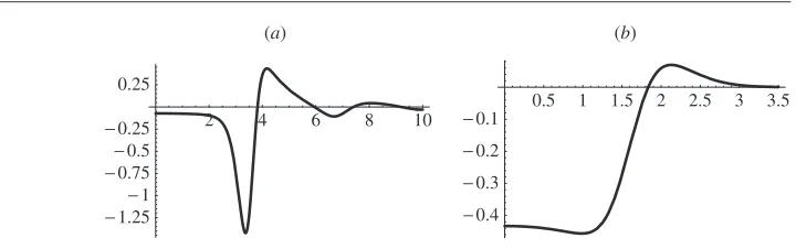
Figure 2. The critical point charge correlation functiongc(r),plotted for two choices ofC(r):
(a)C(r)=J0(r);(b)C(r)=exp(−r2/2).
where the necessary entries ofΞc,are found using Jacobi’s determinant theorem in (A.3); as an example,
24=M0−F I2
F02−F2. (5.9)
The topological charge correlation function gc(r) for critical points is obtained by substituting (5.6), (5.8) (with all terms like (5.9) found using (A.3) into (2.10)). This expression is complicated and not very illuminating, and is not given here. Upon substituting (3.5), (3.6), (5.5) in, one finds thatgccan be written as a perfect derivative (cf (4.8)),
gc(r)= 1 4π2d2
cr dhc
dr (5.10)
where
hc(r)=
(C−C/r)
rC02−C2C2
0 −C2/r2
C(3)3C2
0 −2C2−CC/r
C02−C2
−(C−C/r)
3C2
0 −2C2/r2−CC/r
rC2
0 −C2/r2
= 1
r(C−C/r)
d dr
(C−C/r)3
C02−C2C2
0 −C2/r2
. (5.11)
This process of findinghcis long and tedious, and details are omitted here. It is easy to see thathc→0 asr→ ∞;it is straightforward, by Taylor expanding derivatives ofC,to show that
hc(0)= 4C0(4)
3√3C0 = −2π dc. (5.12)
The critical point topological charge correlation function for two particular field correlation functions is shown in figure2. As with the two-dimensional vector case plotted in figure1, the properties of the correlation function (oscillatory, exponential decay, etc) are similar to that of the underlying field correlation functionC(r), on which the correlation function depends. Features of interest in these plots include the sharp initial minimum of (a), and the fact that the monotonic decay in (b) is from above, not below (in contrast to its counterpart in figure1). Nevertheless, the form ofhcis significantly more complicated than
6. Umbilic points
Less well-known than critical points, umbilic points are geometric point singularity features associated with the second derivative of f—namely where Hessian matrix of second derivatives∂ijf is degenerate (Berry and Hannay 1977, Porteous 2001, Hilbert and Cohn-Vossen 1952). Geometrically, the principal axes of Gaussian curvature are not defined at these points. The eigenvalues of the Hessian coincide whenf,xx =f,yy, f,xy =0.Umbilic points are therefore zeros of the two-dimensional vector field
vu=((f,xx−f,yy)/2, f,xy). (6.1)
The factor of half in the first term ensures thatvuis statistically rotation invariant.
An umbilic point has an index, determined geometrically by the sense of rotation of the principal axes of curvature around the umbilic point, and the index is generically±1/2 (Berry and Hannay 1977); only the sign of the index is of interest here, and this is determined by the appropriate JacobianJuonvu,
2Ju=f,xxxf,xyy +f,yyyf,xxy−f,xyy2 −f
2
,xxy (6.2)
depending on the third partial derivatives of f. The calculation of the topological charge correlation function for umbilic points can proceed according to the scheme of section2, in a similar way to the corresponding calculation for critical points.
Umbilic points for isotropic random functions was considered by Berry and Hannay; they found the densityduto be (Berry and Hannay 1977, equation (34))
du=
3C0(6)
10π C0(4)
(6.3)
(C0(6)is the sixth derivative ofCat 0) and that the average indexqis zero (the separate densities are 0.5dufor stars, 0.05279dufor monstars, and 0.44721dufor lemons). In the present work, the distinction between monstars and lemons, which both have positive index, is not used.
The ordering of the vector of Gaussian random functionsuuis chosen
uu=(fA,xxx, fA,xyy, fB,xxx, fB,xyy, fA,xxy, fA,yyy, fB,xxy, fB,yyy,
(fA,xx−fA,yy)/2, (fB,xx−fB,yy)/2, fA,xy, fB,xy). (6.4)
The correlation matrix (2.2) is
Σu=
S0 T0 S T 0 0 0 0 0 −X 0 0
T0 T0 T U 0 0 0 0 0 −Y 0 0
S T S0 T0 0 0 0 0 X 0 0 0
T U T0 T0 0 0 0 0 Y 0 0 0
0 0 0 0 T0 T0 T U 0 0 0 −Q
0 0 0 0 T0 S0 U V 0 0 0 −R
0 0 0 0 T U T0 T0 0 0 Q 0
0 0 0 0 U V T0 S0 0 0 R 0
0 0 X Y 0 0 0 0 L0 W 0 0
−X −Y 0 0 0 0 0 0 W L0 0 0
0 0 0 0 0 0 Q R 0 0 L0 L
0 0 0 0 −Q −R 0 0 0 0 L L0
(b) (a)
2 4 6 8 10
−0.3 −0.2 −0.1 0.1 0.2
1 2 3 4
[image:12.595.109.468.86.199.2]−0.5 −0.4 −0.3 −0.2 −0.1
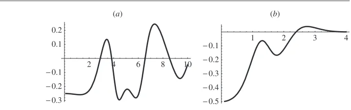
Figure 3. The umbilic charge correlation function gu(r),plotted for two choices ofC(r):
(a)C(r)=J0(r);(b)C(r)=exp(−r2/2).
whereW ≡(M+N−2L)/4, X≡(P −Q)/2, Y ≡(Q−R)/2 and
P ≡ −∂x5Cx=r,y=
0 = −C
(5)
Q≡ −∂x3∂y2Cx=r,y=
0 = −(r 3C(4)−
3r2C(3)+ 6rC−6C)/r4 R≡ −∂x∂y4C
x=r,y=0= −3(r 2C(3)−
3rC+ 3C)/r4
S≡ −∂x6Cx=r,y=0 = −C(6) T ≡ −∂x4∂y2Cx=r,y=
0 = −(r 4C(5)−
4r3C(4)+ 12r2C(3)−24rC+ 24C)/r5 (6.6)
U≡ −∂x2∂y4Cx=r,y=
0= −3(r 3C(4)−
5r2C(3)+ 12rC−12C)/r5 V ≡ −∂y6Cx
=r,y=0 = −15(r 2C(3)−
3rC+ 3C)/r5
P0=Q0=R0 =0 S0=5T0=5U0=V0= −C(06). The matrixKu,defined using (2.5), has determinant
detKu=
L20−(M+N−2L)2/16L20−L2. (6.7)
The result of the Jacobian derivative operators (2.11) gives
Du=212+214+222+ 2224−21222+1324−41424−21255+ 21256 −22256+255+256+ 2257+258−25556−45758+5768.
(6.8)
The necessary entries of Ξu are found using (A.3). The resulting expression for Du,and therefore forgu,is very complicated, but may be reduced to the following form:
gu(r)= 1 4π2d2
ur dhu
dr (6.9)
where
hu(r)= d dr
r(Q−R)2
4√detKu
+Q(P +R−2Q) 4√detKu
. (6.10)
It can be shown thathu(0)= −2π du,andh → 0 asr → ∞. gu(r)is plotted in figure3 forC(r)=J0(r)and exp(−r2/2).The most obvious feature of these two plots, compared to figures1,2, is that they have a negative maximum, a property that seems to be general forgu, although this has not been proved. It is unclear what the physical significance of this kink should be; mathematically, it probably arises from interference between the two summands in
7. Topological charge screening
Three particular charge correlation functions have been derived exactly (equations (4.8), (4.9), (5.10), (5.11), (6.9), (6.10)). In each case, the charge correlation function has the form
g(r)= (n−1)! (2π )nd2rn−1
dh(r)
dr (7.1)
wherenis the number of dimensions,dis the density of zeros andh(r)is a function such that
h(0)= (2π ) nd σn−1(n−1)!
h→ ∞ asr→ ∞. (7.2)
The total charge density around a given (say positive) topological charge is therefore
d
dnrg(r)= (n−1)! (2π )nd σn−1
∞
0
drdh(r)
dr
= (n−1)!σn−1
(2π )nd2 (h(∞)−h(0))
= −1 (7.3)
where the hypersphere areaσn−1appears in the first line from integration in polar coordinates. It implies that the distribution of topological charges is such that every topological charge tends to be surrounded by charges of the opposite sign, such that the topological charge is ‘screened’ at large distances. This fact was noted in the random vector case by Halperin (1981) and Liu and Mazenko (1992) (although the general zero densitydnhad not been determined explicitly) and is independent of the field correlation functionC.The derivation here shows that this is a more general phenomenon, possibly a universal feature of topological charge correlations for Gaussian random fields. It should be noted that (7.3) is not necessarily satisfied for an arbitrary distribution of signed points; for instance,g(r) =0 always for Poisson points, for which there is no screening.δ-function correlations at the origin are ignored in the following. An analogy may be drawn from the theory of ionic liquids (Hansen and McDonald 1986); in a fluid or plasma, consisting of two species identical except for opposite (Coulomb) charges, the following Stillinger-Lovett sum rules (Stillinger and Lovett 1968a,1968b) are found to hold:
d
dnrg(r)= −1 (7.4)
d
dnrr2g(r)= −an2. (7.5)
Here, g is the charge–charge correlation function, is a characteristic screening length dependent on temperature andn,andanis a constant dependent on dimensionality. These rules are discussed forn=3 by Hansen and McDonald (1986), Stillinger and Lovett (1968a,1968b), andn=2 by Jancovici (1987), Jancoviciet al(1994).
The screening relation (7.3) is equivalent to the first Stillinger–Lovett sum rule (7.4), which is derived using the statistical mechanics of pairwise, Coulomb interacting fluids. It is unclear whether the fact that topological and Coulombic charges screen in the same way is coincidence, or evidence of some deeper connection between the two statistical theories.
It is natural to ask whether the topological charge correlation functions satisfy the second sum rule, which (upon integrating the left-hand side of (7.5) by parts), depends on the integral ofrh.Forn= 2,it was found (Berry and Dennis 2000) that for certain choices ofC,this integral may diverge. The slowest decay comes whenC =J0,and by (4.9),
giving a logarithmic divergence for the second moment. For comparison, the critical and umbilic functions hc, hu, (equations (5.11), (6.10), respectively) both give, for the same choice ofC,
hc(r), hu(r)∼r→∞cos(2r)/r2 when C=J0 (7.7)
implying that the second sum rule is satisfied generally for critical and umbilic points, although, as for the cases of random vectors where the integral converges, the screening length,defined in analogy to (7.5), depends on the choice ofC.For random vectors withn >2,the second moment ofgalways converges, because of the higher power ofCappearing in (4.9) (also, the decay ofCwill be faster, as discussed at the end of section3).
Comparison may be drawn to the electrostatic analogy in random matrix theory, particularly in the case of the so-called Ginibre ensemble ofN×N matrices whose entries are independent, identically distributed circular Gaussian random variables (Ginibre 1965). The eigenvalues of these matrices are found to have exactly the same statistical behaviour as a 1-component two-dimensional Coulomb gas of N charges in a harmonic oscillator potential, and the 2-point density correlation function screens against a uniform background (i.e.,d d2z(g
Gin−1)= −1), and have finite second moment. Certain random polynomial analogues have zeros that can also be expressed as two-dimensional Coulomb gases with additional interactions (Hannay 1998, Forrester and Honner 1999). The eigenvalues of random matrices (which may be expressed as the zeros of the characteristic polynomial) and zeros of random polynomials are all of the same sign, since they are zeros of complex analytic functions, and the density correlation functions of zeros are unique (there is no analogue ofC).
There may be a danger in taking the analogy with fluids too far; for instance, the oscillations of the functions in figures 1–3(a) are reminiscent of those of charged fluids (e.g., Hansen and McDonald (1986)). However, the physical causes for these oscillations are very different. In fluids, the oscillations usually arise from packing considerations (the ions themselves are of finite size, fixing the lengthscale, although in plasmas they are usually represented as point charges (Baus and Hansen 1980)). Topological charges, on the other hand, are points, and the oscillations in these figures originate from the oscillations in the underlying field correlation functionC(r),which isJ0in this case. Although Halperin (1981) discusses the similarity between the short-range behaviour of the two-dimensional vector correlation function (4.8), (4.9) and Kosterlitz–Thouless theory, the present situation is more general, both in that the (possibly long-range) screening is exact, and that the results hold for any reasonable field correlation functionC(r).
8. Discussion
Using a general scheme for calculating topological charge correlation functions, three particular correlation functions were found explicitly, and were found always to satisfy a screening relation (7.3).
The scheme of section 2 used to calculate the charge correlation functions is very general, and can be generalized to calculate the charge–charge correlation function between two different sets of topological charges—for instance with a critical point at A, and an umbilic point atB. Although not done so here, the scheme may be applied to anisotropic fields.
two-dimensional vectors (realized as complex scalars) by Berry and Dennis (2000), Saichev
et al(2001). However, it has not been possible to generalize such methods to the case of critical points. Also, numerical evidence (Freund and Wilkinson 1998) suggests that the correlation function of extrema signed by the sign of their laplacian (+1 for minima,−1 for maxima) also satisfies the screening relation (7.4). All such functions would be needed to calculate the partial correlation functions between the species (e.g., maxima with maxima, maxima with saddles, maxima with minima, etc), which would give a complete statistical picture.
The presence of boundaries in the random function will affect the statistical properties of topological charges (e.g., Berry (2002) for nodal points in the plane), and it is possible that there may be some further analogy with the physics of interfaces of Coulomb fluids. The scheme of section2 ought to be adaptable to calculate charge correlation functions in this case.
Only zeros of fields linear in Gaussian random functions have been considered here, although the density of others may be calculated, for instance, in addition to nodal points, a two-dimensional Gaussian random complex scalar has critical points of its modulus squared (Weinrib and Halperin 1982) and its argument (Dennis 2001a). The scheme employed here cannot be used to calculate correlation functions for these, although numerical evidence (I Freund, personal communication) suggests that the critical points of argument (together with the nodal points) do screen, therefore adding to the cases shown here. It is tempting to conjecture that topological charge screening may be a universal phenomenon in Gaussian random fields.
Acknowledgments
I would like to thank Michael Berry and Robert Evans for useful discussions, John Hannay for discussions leading to the arguments in appendix B, and Isaac Freund for correspondence. This research was supported by the Leverhulme Trust.
Appendix A. Jacobi’s determinant theorem
LetAbe a square matrix. TheminorMi1...ik
j1...jk(A)is the determinant of thek×ksubmatrix
ofAwith rowsi1, . . . , ik and columnsj1, . . . , jk. M i1,...,ik
j1,...,jk(A)shall be used to denote the
complementary minor, that is, the minor of the submatrix of A with rowsi1, . . . , ik and
columnsj1, . . . , jnexcluded. Then Jacobi’s determinant theorem (Jeffreys and Jeffreys 1956, p 135) states
detAMi1,...,ik j1,...,jk(A
−1)=(−1)i1+···+ik+j1+···+jkMi1,...,ik
j1,...,jk(A). (A.1)
Applying this to Σin (2.5), and choosingΞ−1 as the submatrix whose determinant is the minor ofΣ−1,
detΣdetΞ−1=detΣM11,...,,...,22mm(Σ−1)
=(−1)1+···+2m+1+···+2mM22mm+1+1,...,,...,22(m(m++n)n)(Σ)
=detK (A.2)
from which (2.6) follows directly.
Ξ−1,and once onΣ.Therefore,
ij =Mij(Ξ)
=(−1)i+jMji(Ξ−1)/detΞ−1
=(−1)i+jdetΞM11,...,j,...,i−−11,i,j+1+1,...,,...,22mm(Σ−1) =detΞMi,j,22mm+1+1,...,,...,22mm+2+2nn(Σ)
=Mi,2m+1,...,2m+2n
j,2m+1,...,2m+2n(Σ)/detK =detK−1det
ij •
• K
(A.3)
where in the last line•represents the termsi,k, k,j wherek=2m+ 1, . . . ,2m+ 2n.Thus theijappearing in the expression forDin (2.12), is the determinant of the(2n+ 1)×(2n+ 1)
submatrix comprised of theith row andjth column ofΣ,and the submatrixK.
Appendix B. Calculation of the density of vector zeros (4.1)
In order to integrate (4.1), the following must be integrated
V=
dn2vi,j|detvi,j|exp
−1
2
n
i,j=1
v2i,j
. (B.1)
This is, mathematically, the average hypervolume of ann-dimensional parallelepiped specified by Gaussian random vectors w1 = (v1,1, . . . , v1,n), . . . ,wn = (vn,1, . . . , vn,n). These Gaussian random vectors are identically distributed isotropically in n-dimensional space. The hypervolume is nonzero exactly when the set ofnvectors is linearly independent.
This hypervolume may be found explicitly in a manner reminiscent of the Gram–Schmidt orthogonalization procedure for vectors. Geometrically,
volume of parallelepiped=length ofw1× length ofw2orthogonal tow1× · · ·
×length ofwnorthogonal to span{w1, . . . ,wn−1}. (B.2)
A given factor in this product is therefore the average length of the Gaussian random vector wj in the orthogonal complement of a(j−1)-dimensional subspace span{w1, . . . ,wj−1}.
Now, since the vectorwj is isotropic, it may be represented identically in any choice
of orthonormal basis of n-dimensional space; in particular, its first j −1 components
vj,1, . . . , vj,j−1 may be chosen to be in span{w1, . . . ,wj−1} (as in the Gram–Schmidt procedure). The total contribution ofwj to the integral in (4.1) involves the average length of
the vector made up of the other componentsvj,j, . . . , vj,n.Wherek=n−j−1,this is
dnwj
vj,21+· · ·+v2j,nexp
−1
2
n
i=1
v2j,i
= ∞
−∞d
vj,1exp
−v2j,1/2!
j−1
Sk−1
dk−1k−1
∞
0
dρ ρkexp(−ρ2/2) (B.3)
coordinates, with dωk−1the solid angle infinitesimal on the unit(k−1)-sphereSk−1,andρis the radius. It is well known that the surface areaσk−1of the unit(k−1)-hypersphere is
σk−1=
dk−1k−1= 2πk/2
k−2
2
!. (B.4)
The ρ integral in (B.3) is 2(k−1)/2((k −1)/2)!. Therefore, the numerical part of (4.1) is 1/(2π )n(n+1)/2times the product in (B.2), with each term in the product, now labelled byk,
given by the expression (B.3). Therefore,
V= 1
(2π )n(n+1)/2
n
k=1
(2π )(n−k)/2× 2π k/2
k−2
2
!×2
(k−1)/2
k−1
2
!
= 1
(2π )n(n+1)/2
n
k=1
(2π )(n+1)/2πn/2 k−1
2
!
k−2
2
!
= n−1
2
!
π(n+1)/2. (B.5)
This value agrees with that stated by Halperin (1981), Liu and Mazenko (1992) of 1/π (n=1), 1/2π (n=2)and 1/π2(n=3).
References
Adler R J 1981The Geometry of Random Fields(New york: Wiley)
Baus M and Hansen J-P 1980 Statistical mechanics of simple Coulomb systemsPhys. Rep.591–94 Berry M V 1977 Regular and irregular semiclassical wavefunctionsJ. Phys. A: Math. Gen.102083–91
Berry M V 1978 Disruption of wavefronts: statistics of dislocations in incoherent Gaussian random wavesJ. Phys. A: Math. Gen.1127–37
Berry M V 2002 Statistics of nodal lines and points in quantum billiards: perimeter corrections, fluctuations, curvature
J. Phys. A: Math. Gen.353025–38
Berry M V and Hannay J H 1977 Umbilic points on a Gaussian random surfaceJ. Phys. A: Math. Gen.101809–21 Berry M V and Dennis M R 2000 Phase singularities in isotropic random wavesProc. R. Soc.A4562059–79 Berry M V and Dennis M R 2000 Phase singularities in isotropic random wavesProc. R. Soc.A4563059 (errata) Dennis M R 2001a Phase critical point densities in planar isotropic random wavesJ. Phys. A: Math. Gen.34
L297–L303
Dennis M R 2001b Topological singularities in wave fieldsPhD ThesisBristol University
Dennis M R 2002 Polarization singularities in paraxial vector fields: morphology and statisticsOpt. Commun.213 201–21
Feller W 1950An Introduction to Probability Theory and Its Applicationsvol 1 (New York: Wiley)
Foltin G 2003a Signed zeros of Gaussian vector fields—density, correlation functions and curvatureJ. Phys. A: Math. Gen.361729–41
Foltin G 2003b The distribution of extremal points of Gaussian scalar fieldsJ. Phys. A: Math. Gen.364561–80 Forrester P J and Honner G 1999 Exact statistical properties of complex random polynomialsJ. Phys. A: Math. Gen.
322961–81
Freund I and Wilkinson M 1998 Critical-point screening in random wave fieldsJ. Opt. Soc. Am.A152892–902 Ginibre J 1965 Statistical ensembles of complex, quaternion and real matricesJ. Math. Phys.6440–9
Halperin B I 1981 Statistical mechanics of topological defects Les Houches Session XXV—Physics of Defects
ed R Balian, M Kl´eman and J-P Poirier (Amsterdam: North-Holland) Hannay J H 1998 The chaotic analytic functionJ. Phys. A: Math. Gen.31L755–61 Hansen J-P and McDonald I R 1986Theory of Simple Liquids(New York: Academic) Hilbert D and Cohn-Vossen S 1952Geometry and the Imagination(New York: Chelsea)
Jancovici B 1987 Charge correlations and sum rules in Coulomb systems: IStrongly Coupled Plasma Physics
ed F J Rogers and H E Dewitt (New York: Plenum)
Jancovici B, Manificat G and Pisani C 1994 Coulomb systems seen as critical systems: finite-size effects in two dimensionsJ. Stat. Phys.78307–29
Liu F and Mazenko G F 1992 Defect–defect correlation in the dynamics of first-order phase transitionsPhys. Rev.B 465963–71
Longuet-Higgins M S 1957a The statistical analysis of a random, moving surfacePhil. Trans. R. Soc.A249321–87 Longuet-Higgins M S 1957b Statistical properties of an isotropic random surfacePhil. Trans. R. Soc.A250157–74 Longuet-Higgins M S 1958 The statistical distribution of the curvature of a random Gaussian surfaceProc. Camb.
Phil. Soc.54439–53
Mermin N D 1979 The topological theory of defects in ordered mediaRev. Mod. Phys.51591–648 Milnor J W 1965Topology from the Differentiable Viewpoint(Charlottesville, VA: Virginia University Press) Nye J F and Berry M V 1974 Dislocations in wave trainsProc. R. Soc. A336165–90
Porteous I R 2001Geometric Differentiation: For the Intelligence of Curves and Surfaces2nd edn (Cambridge: Cambridge University Press)
Rice S O 1954 Mathematical analysis of random noiseSelected Papers on Noise and Stochastic Processesed N Wax (New York: Dover)
Saichev A I, Berggren K-F and Sadreev A F 2001 Distribution of nearest distances between nodal points for the Berry function in two dimensionsPhys. Rev.E64036222
Stillinger F H and Lovett R 1968a Ion-pair theory of concentrated electrolytes. I. Basic conceptsJ. Chem. Phys.48 3858–68
Stillinger F H and Lovett R 1968b General restriction on the distribution of ions in electrolytesJ. Chem. Phys.49 1991–4