Abstract—Extensive proportions of active water distribution networks are situated in urban regions with very high service demands that subject them to lots of external pressure. This means that they are exposed to higher risks-of-failure. Within urban regions, however, water pipelines are lined in different city locations with varied risk levels. Pipelines are bound to fail despite their location. Nonetheless, additional location dependent risk elements may either heighten or lower the failure process. In this paper therefore, we evaluate failure trends of pipelines in a region characterized with two soil types; regular and volatile Dolomitic grounds, outlining how the different soil types affect water pipeline failures. We also assess failure variations in two major pipe alignment zones identified during the study. To achieve this, we used data from a selected metropolitan region in South Africa and applied Bayesian Networks to accommodate inherent data uncertainty while modeling failure causal properties. Findings from the assessment indicate that risk-of-failure is higher along exit sections that experience additional external pressure.
Index Terms—water distribution networks, leakage, water pipeline failure, Bayesian networks, risk-of-failure.
I. INTRODUCTION
Ortable water infrastructure varies from small straightforward rural gravity systems to more complicated and computerized schemes with numerous distribution networks in larger cities [1]. In urban regions, however, distribution networks are exposed to increased levels of operational pressure considering the magnitude of workload in these areas. In South Africa, practically all the metropolitan regions undergo rapid population growth rates of about 4.3% on an annual basis. In addition to this, there is an even higher increase in the number of water dependent economic activities [2]. Besides the build up of demands in urban areas; pipelines are also subjected to a continuous decomposition process that is heavily influenced by surrounding environmental conditions [3]. Consequently, as a steady pipeline disintegration process carries on in the
Manuscript received November 2, 2017; revised January 12, 2018. This work was supported in part by the South Africa, National Research Foundation under Grant No. 105808.
Achieng G. Ogutu is with Department of Computer Science, ICT Faculty, Tshwane University of Technology, Private Bag X680, Pretoria 0001, South Africa ([email protected]).
Okuthe P. Kogeda is with Department of Computer Science, ICT Faculty, Tshwane University of Technology, Private Bag X680, Pretoria 0001, South Africa ([email protected]).
Manoj Lall is with Department of Computer Science, ICT Faculty, Tshwane University of Technology, Private Bag X680, Pretoria 0001, South Africa ([email protected]).
midst the ever increasing urban pressure, increased pipeline failures are witnessed. This has increased awareness about the need for better management of water infrastructure, which in turn, results to the development of research based and techniques of assessing pipeline operation, maintenance as well as pipeline failure [3], [4].
Pipeline failures are generally referred to as the ‘unintended loss of pipeline contents’ [5], Pipeline failures are inevitable [1], [4] and appear in different forms [1], including pipe breaks [4], [6], [7], cracks along the pipelines [8], pipe bursts [9] –[12] or even total collapse after extended exposure to extreme conditions [13]. Regardless of the type of failure, their effects stretch over the entire community, its environment and even affect human health and wellness [1], [3], [14], and [15]. If these failures occur in unstable Dolomitic grounds like in our study area, then the effects could be fatal. Active preventative measures are therefore encouraged to assist in minimization of pipeline failures. This can be achieved through prediction of failure possibilities along the distribution networks.
II. DOLOMITIC GROUNDS AND PIPELINE FAILURES
Dolomitic grounds are regions with an undercover of dolomite rocks [16], [17]. These regions are highly unstable (volatile) and are generally considered as high-risk locations [17], [18]. Dolomite rocks can dissolve in water [16]-[19], and when this happens, hollow spaces are created within them. Top soil coverage is then compelled to cave in to fill the hollows leading to massive ground movements that cause immense structural damage [16], [17]. This makes them potentially dangerous locations in cases of pipeline leakage. On the other hand, with their composition of a carbonate of magnesium and calcium, the rocks act as neutralizing agents with only 4% corrosion effect on pipelines [20]. Given that corrosion is a major contributor to pipeline failure [1], [7], [21], and [22], dolomite rocks therefore, have a possibility of minimizing pipeline failure. This however, does not dismiss the collapsible tendencies of soil in such regions [16]-[19], which may result in cracking and breaking of pipelines. In addition, longitudinal and circumferential deflections as well as the safe span space of pipelines are also considered to greatly influence failure in these grounds [14], [23]-[25]. For this reason, it is very important to identify the trends of failure in such regions, with the aim of utilizing these trends in constructive leakage prediction modeling.
A Probabilistic Assessment of Location
Dependent Failure Trends in South African
Water Distribution Networks
Achieng G. Ogutu, Okuthe P. Kogeda, and Manoj Lall
III. UNCERTAINTY IN HISTORICAL FAILURE RECORDS
During the process of modeling, uncertainty can be encountered in various ways, including irregularities in analysis and parameterization [26], [27], model extraction and integration processes [28], as well as uncertainty with the data itself [26], [27], [29]. This study, however, focuses on the aspect of data uncertainty. Historical records about failures and maintenance procedures are used for model creation and testing purposes. These records, mostly obtained from water utilities have the tendency of being deficient or full of flawed information, or sometimes, both [23], [28]. In addition, different techniques used for data acquisition may also produce results with a number of assumptions that may threaten the integrity of the data collected [30]. Therefore, historical data may be highly uncertain, causing substantial complications during estimation of pipeline failure trends [28], [31]. In extreme situations, some utilities may not even have data completely [23], [31], and [32]. These uncertainties can however, be accommodated into modeling, through the use of dynamic models that can assimilate both prior knowledge and collected data [28], [33]. One such technique is Bayesian Networks (BNs). Other techniques, fit for handling data uncertainty are highlighted in the following Sub Section 3.1.
A. Techniques for Handling Data Uncertainty
Effective manipulation of historical data with uncertainty in a predictive modelling process ought to capture every single aspect of data dependency, especially based on causal perspective; an aspect assumed by most models [30], [33], and [34]. Utilization of network-based models may therefore, be effective for capturing data dependency, making it easier to deal with inherent data uncertainty. Some of these network based modelling techniques, as discussed in [33] include: Cradle Networks (CNs), Cognitive Maps, also called Fuzzy Cognitive Maps (CM/FCM), Bayesian Belief Networks (BBNs), Fuzzy Rule Based Models (FRBM), Analytic Network Process (ANP) and Artificial Neural Networks (ANN). Additionally, a comparison of these techniques based on their ability to handle data uncertainty and several other modelling qualities such as complexity, scalability, ability to handle different inputs among others, is also performed [33]. In consideration to the techniques highlighted herein, this research makes use of Bayesian Networks (BNs).
B. Bayesian Network for Pipeline Failure
Bayesian Networks (BNs) are sometimes referred to as Belief Networks or Directed Acyclic Graphs (DAG). They are built using nodes that symbolize practical variables in a system; and arcs that join the nodes, demonstrating probabilistic relationships among them [27], [35]. The nodes and arcs are ordered and connected strategically indicating causal relationships between the variables, which creates generational problem solutions, whereby a node is referred to as a child or parent of another node [28].A parent node is a node that directly influences the occurrence of another node, which becomes its child. Parent nodes are, considered as the event originators in a BN domain [28], [36]. If a node does not have any children however, it is given the name
result [36]. Non-root and non-leaf nodes are known as intermediate nodes.
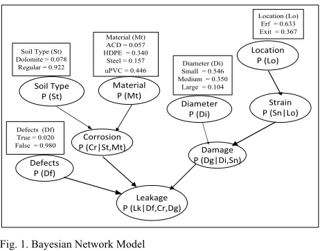
Causal dependency in a BN domain is effected through direction of connectivity between the nodes in the sense that the node to which an arc is extended become the child of a node from where the arc is extended [28], [33]. Uncertainty is accommodated through assignment of relevant probabilities to the model variables [36], which are computed to achieve the overall result using Bayes theorem as given by equation (1). A BN model for leakage detection is illustrated in Fig.1.
) (
) | ( ) ( ) | (
y P
y P P y
Pθ = θ θ (1) Where θ is the unknown variable under estimation, P (θ|y),the posterior probability of θ, P(θ) giving the prior likelihood θ and P(y|θ) as the likelihood function for any chance of occurrence of state y considering available alleged causal dependencies and the predictive parameters.
C. Why Bayesian Networks?
Based on a comparison of the techniques discussed in Section 3.1, BNs stand out as a suitable candidate for modelling pipeline failures based on its qualities such as ability to express data causality even in qualitative inputs. In addition to this, BNs also have the ability to handle small and incomplete data sets. Using BNs, it is possible to model scalable complex systems; but at the same time, allow speedy outlay of results. Most importantly however, is their ability to combine knowledge from several sources and how well they accommodate explicit treatment of uncertainty. BNs, however, require data to be effective and also require skill and knowledge to work with. Although BNs have been used to model pipeline failures in a number of instances, majority of the models produced somehow lack location specificity, especially in high-risk zones. This is adequately addressed in this study.
D. Overview of application of Bayesian Networks to Model Pipeline Failures
BNs have been applied in several ways to model different aspects of pipeline failures in general [26], [27], [37]-[40]. While undertaking a research aimed at assessing the risk of failure of metal pipelines, BNs were used to accommodate the combination of a number of dissimilar factors of failure in [33]. Bayesian inference was then used to evaluate and determine possibility of failure in these pipes. Similarly, a research aimed at identifying the extent to which various causal factors influence failure was conducted in [37]. In this research, BNs was used to compute the weight of influence of these factors to failure, after which, the results were used to calculate the deterioration rates of water pipelines.
combinations showcase the flexibility of BNs indicating various possibilities on how BNs can be employed in leakage prediction.
IV. DATA DESCRIPTION AND FINDINGS IN THE STUDY AREA
Situated in a moderately populated urban setting, Doringkloof suburbs in Gauteng Province, South Africa have a number of activities underweight, including an active process of pipeline rehabilitation activities. Data pertaining to pipeline failure and maintenance for a period of 5 years, as well as data about the pipeline (asset) details in the region were obtained from the municipal water department. The sets of data were then analyzed and merged together so as to obtain the variables used in the BN model in Fig. 1. From the data, we identified that selected area has over 1,000 pipeline connections. Over the stated duration, approximately 335 leakage episodes were recorded, with 58% of the failures requiring repairs of water distribution pipes. An illustration of this observation is given in Fig. 2, in Section 5.
Majority of the repairs were conducted on small pipes with diameters of about 100mm. On the other hand, the least number of repairs were conducted on large pipes, with diameters of between 350-600mm, confirming that small diameter pipes are more prone to failure than pipes with larger diameters [9], [41], and [42] as illustrated in Fig. 3 in Section 5. Pipe age was found to considerably affect failure, derived from the fact that majority of pipe failures was observed in pipes that were laid down in the period between the late 1960s and late 1970s. This is the period when the oldest pipes in the region were identified.
We also discovered that majority of failures recorded were concentrated along street corners and road intersections, also referred to as Exit Roads. This element may be as a result of added external stress imposed on the pipes [20]-[22]. This is the hypothesis that we seek to prove in this paper through the use of Bayesian Networks.
A. The Failure Prediction Model
For model creation, we made use of 8 factors that adequately exhibit causal tendencies including: Location (Lo), Strain (Sn), Soil-type (St), Material (Mt), Corrosion (Cr), Diameter (Di), Damage (Dg), and Defects (Df). Based on literature, their ability to influence favourable conditions that either cause, or lead to pipeline deterioration and eventual failure were determined. Although pipe Age may highly influence pipeline failure, it does not reveal direct causal effect to other variables; hence it is excluded from the model.
Using these variables, the BN structure was developed as shown in Fig. 1; with the Conditional Probability Tables of the root nodes as well as the conditional probability distributions for the intermediate variables specified as indicated in the Conditional Probability Tables (CPTs) shown in Tables I to IV.
Material P (Mt)
Diameter P (Di) Soil Type
P (St)
Defects P (Df)
Corrosion
P (Cr|St,Mt) Damage P (Dg|Di,Sn)
Leakage P (Lk|Df,Cr,Dg)
Strain P (Sn|Lo) Location
P (Lo) Soil Type (St)
Dolomite = 0.078 Regular = 0.922
Material (Mt) ACD = 0.057 HDPE = 0.340
Steel = 0.157 uPVC = 0.446
Diameter (Di) Small = 0.546 Medium = 0.350
Large = 0.104
Location (Lo) Erf = 0.633 Exit = 0.367
Defects (Df) True = 0.020 False = 0.980
[image:3.595.315.546.48.229.2]
Fig. 1. Bayesian Network Model
In Fig. 1, the uppermost parameters (Soil-Type, Material, Diameter, and Location) as well as Defects; are the independent root nodes. The type of Material that the pipe is made up of as well as the Soil Type where the pipe is laid influences the occurrence of corrosion in a pipe. The location of a pipe on the other hand, determines how much Strain it would undergo. Strain acts collectively with Diameter to cause pipeline Damage. A walk through the genealogical causal relationship leads us to leakage, which is the ultimate goal of the system. Leakage is influenced by the presence of Damage in a pipe, Corrosion as well as Defects. Initial probability distributions for all the nodes, also referred to as prior probabilities, were generated from the data set, literature and in some instances, through expert elicitation.
Based on the number of present variables, the joint probability P (XI, X2,…, Xn) of any set of variables in the
domain is generated for effective evaluation of the target node. This is achieved by getting the product of all available distributions for every variable in the in the domain [36, 43]. However, if variables {Xi,…..Xk} ∈ {X1, X2,…,Xn} constitutes
a particular set of variables Y⊂X and takes on the arrangement y = {Xi =xi,…Xk = xk}, then the probability of y
is obtained by getting the sum of all the joint probabilities of X in the distribution of Xi =xi,… Xk =xk [43], [44].
Because BN are updated based on acquisition of new evidence pertaining to the variables, then if we acquire a new group of evidence e, given as e = {Xi =xi,…Xk = xk},
that are contained by all the acknowledged values of the random variables in a BN, of which {Xi, …, Xk} ⊂ {X1, X2,…, Xn}, then computation of the probability of a variable
Xt, when Xt ∉{Xi, …, Xk} assumes the value xt as shown in
equation (2), which is basically derived from equation (1) [43]- [46].
) (
) | ( ) ( ) | (
e P
x x e P x x P e x x
P t t t t
t t
= ×
= =
= (2)
For instance, in Fig. 1, if we observe evidence that a pipe is made of Dry Asbestos Cement (ACD) pipe material, our evidence e = {Mt = ACD}, then belief that there is corrosion would be given as:
) (
) ,
( |
(
ACD Mt P
ACD Mt Yes Cr P ACD Mt Yes Cr P
= = =
= =
= (3)
of failure given the conditions is computed as in equation (4)
TABLE I: Conditional Probability Table (CPT) for Strain (Sn)
Location (Lo) Probability of Strain (Sn)
High Low NoStrain
Erf 0.120 0.520 0.360
[image:4.595.304.548.222.337.2]Exit 0.640 0.200 0.160
[image:4.595.41.259.324.489.2]TABLE II: Conditional Probability Table (CPT) for Corrosion (Cr)
TABLE III: Conditional Probability Table (CPT) for Damage (Dg)
TABLE IV: Conditional Probability Table (CPT) for Leakage (Lk)
) ,
, ,
(
) ,
, ,
, (
Erf Lo Small Di ACD Mt Dol St P
Erf Lo Small Di ACD Mt Dol St Pos Lk P
= =
= =
= =
= =
= (4)
Equation (4) is used to compute failure probabilities for different locations, that is, in Erfs and Exit roads. Erfs are pipe alignment regions found within residential areas that are less prone to several activities. Exit locations on the other hand, are regions often exposed to a lot of eternal pressure due to proximity to traffic intersections, round about areas or even busy highways.
V. TESTING AND RESULTS
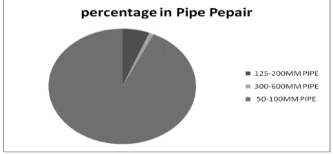
In this Section, we give two sets of results. Firstly, a brief description of some of the observations made from the data set is outlined, and last but not least, we present the BN computation results regarding the effects of location on pipeline failures. There are a number of components that make up a water distribution system including hydrants, valves, and pipelines among others, which are all prone to failure. Of all the leakage related repairs recorded in our data set, their distributions were as illustrated in Fig.2. Majority of repairs were on small diameter pipelines, followed by repairs in the utilities’ service pipes. Least repairs were performed on air valves as well as on large diameter water pipelines.
Fig. 2. Ration of leakage related repairs in the distribution network.
Collectively, most failures were seen on the distribution pipelines, with smaller diameters of between 50mm to 100mm. The larger diameter pipelines of between 300mm to 600mm experienced the least number of leakage related repairs as illustrated in Fig. 3.
Fig. 3. Distribution of leakage repairs based on diameter size of the pipelines
According to Fig. 3, leakage repairs along small diameter pipes accounts for 93% of the total repairs conducted water pipelines only. On the other hand, large diameter pipe failure accounted for just 1% of the total pipeline network repairs recorded.
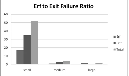
To determine the failure distribution based on pipeline location, a sample space of about 60 pipelines of different sizes in the network were evaluated. From the sample size, failure distribution with regards to the pipe alignment zones was as shown in Fig. 4. This could be explained based on the relationship between external pressure and pipeline failures; in that the greater the exposure to more external pressure, the higher the probability of risk-of-failure [45]-[46]. There were no large diameter pipelines aligned in Exit regions from the sample space, thence the absence of failure record in exit the location.
Material ( Mt)
Soil type (St)
Probability of Corrosion (Cr)
Yes No
ACD Dolomite 0.040 0.960
ACD Regular 0.290 0.710
HDPE Dolomite 0.000 1.000
HDPE Regular 0.000 1.000
Steel Dolomite 0.040 0.960
Steel Regular 0.290 0.710
uPVC Dolomite 0.000 1.000
uPVC Regular 0.000 1.000
Strain ( Sn)
Diameter (Di)
Probability of Damage (Dg)
Yes No
NoStrain Small 0.120 0.880
NoStrain Medium 0.027 0.973
NoStrain Large 0.025 0.975
Low Small 0.160 0.840
Low Medium 0.120 0.880
Low Large 0.080 0.920
High Small 0.640 0.360
High Medium 0.520 0.480
High Large 0.440 0.560
Damage ( Dg)
Corrosion (Cr)
Defects (Df)
Probability of Leakage (Lk)
Positive (Po)
Negative (N)
No No False 0.000 1.000
No No True 0.020 0.980
No Yes False 0.012 0.988
No Yes True 0.050 0.950
Yes No False 0.500 0.500
Yes No True 0.500 0.500
Yes Yes False 0.512 0.488
[image:4.595.306.548.421.533.2] [image:4.595.41.296.508.650.2]Fig. 4. Distribution of failures based on pipeline location.
A. Computation based Results
To illustrate how the joint distribution is used to compute new beliefs about a variable, we make use of Fig. 1, taking into consideration only a small portion of network. We consider a domain made of Soil-Type (St), Material (Mt) and Corrosion (Cr). The joint distribution is given as P (St, Mt, Cr). If expanded, the distribution is expressed as:
) , | ( ) ( ) ( ) , ,
(St Mt Cr P St P Mt PCr St Mt
P = × × (5)
Therefore, if we know that the Soil-Type is Regular, Material is Steel, and Corrosion Positive, then the joint probability of the domain under any circumstances is computed as follows indicated below. It is important to note that P (Cr = Yes| St = Regular and Mt = Steel) = <0.290>given a direct reading from the CPTs for intermediate node (Corrosion).
P (St = Regular, Mt = Steel, Cr = Yes) = P (St = Regular) ×
P (Mt = Steel) × P (St = Regular, Mt = Steel, Cr =Yes)
= 0.922 × 0.157 × 0.290 = 0.04198 ≈ 4.198%
In this instance, the probability of occurrence of Corrosion in a pipeline when pipe material is made of steel and it is installed in a regular piece of land, collectively, becomes 4.198%. The joint probability in this case presents the probability of occurrence of the query node under any circumstance, but within the specified states of the local domain.
During the computation process, the probability of failure in an internal location (Erf) produced the results below: Note that due to the very lengthy nature of the extrapolations of the conditional probability distributions of the variables, entire calculation is not indicated in this paper.
) ,
, ,
(
) ,
, ,
, (
Erf Lo Small Di ACD Mt Dol St P
Erf Lo Small Di ACD Mt Dol St Pos Lk P
= =
= =
= =
= =
=
0.0001783 / 0.0015366 = 0.11604 ≈ 11.604%
On the contrary, probability of failure in a pipeline with the same properties under similar conditions, but in an Exit location with more external pressure resulted to:
) ,
, ,
(
) ,
, ,
, (
Exit Lo Small Di ACD Mt Dol St P
Exit Lo Small Di ACD Mt Dol St Pos Lk P
= =
= =
= =
= =
=
=0.00022325 / 0.0008909 = 0.25059 ≈ 25.059%
[image:5.595.303.553.72.186.2]A visual comparison of the two computations is illustrated in Fig. 5.
Fig. 5. Risk-of-failure margin between Exit and Erf Locations
Based on the comparison of failure probabilities in the two regions as observed from the computations and the chart illustration in Fig.5, there is a 13.455% margin between failure in an Erf and Exit location. This computational outcome verifies the observe outcome in our data analysis process in Section 4, backed up by the illustration in Fig. 4, concerning the differences in failure risk based on location of a pipeline. Additionally risk-of-failure is found to be higher in regions with regular soil types compared to those with dolomite soil type.
VI. CONCLUSIONS
In this paper, an assessment on how the aspect of location affects failure of water pipelines was presented. The process was achieved through an examination of a data set accompanied by predictive investigation through Bayesian Networks. Results from both analyses indicate that majority of pipeline failures arise in regions that are more exposed to higher external pressure.
Besides the findings regarding pipe location and failure, we also realized that the issue of data ambiguity seemed quite unavoidable even though the set of data used was derived from a specific environmental background with the aim of minimizing potential data variations. The noticeable absence of both asset information and maintenance records in some instances showcase the importance of tracking historical failures by respective pipeline utilities.
The model developed herein, made use of only the noticeable causal aspects of pipeline failures. However, to achieve more effectiveness in development of failure prediction models, inclusion of the consequence index that adequately captures the severity of pipeline failures together with tangible estimations of the cost of pipeline failures ought to be considered. This would ensure optimization of the prediction models. We therefore campaign for future research focused on the inclusion of the impacts of pipeline failures to enhance the performance of the failure prediction models.
ACKNOWLEDGMENT
REFERENCES
[1] KLEINER, Y. & RAJANI, B. 2000. Considering time-dependent factors in the statistical prediction of water main breaks. Paper
presented at the Proc., American Water Works Association
Infrastructure Conference. [Accessed: 2015].
[2] STATSSA. 2012 Census 2011 Statistical release. Pretoria, South Africa: Statistics South Africa.
[3] YAMIJALA, S. 2007. Statistical estimation of water distribution system pipe breaks risk. Master of Science, Texas A&M University.
[4] MAKAR, J. M. & KLEINER, Y. 2000. Maintaining water pipeline
integrity. Baltimore, Maryland
[5] MUHLBAUER, W. K. 2004. Pipeline risk management manual: ideas, techniques, and resources. Gulf Professional Publishing. [6] KETTLER, A. & GOULTER, I. 1985. An analysis of pipe breakage
in urban water distribution networks. Canadian Journal of Civil Engineering, 12(2):286-293.
[7] MORRIS, R. 1967. Principal causes and remedies of water main breaks. Journal (American Water Works Association), 59(7):782-798.
[8] IYER, S. & SINHA, S. K. 2005. A robust approach for automatic detection and segmentation of cracks in underground pipeline images.
Image and Vision Computing, 23(10):921-933.
[9] BOXALL, J., O'HAGAN, A., POOLADSAZ, S., SAUL, A. &
UNWIN, D. 2007. Estimation of burst rates in water distribution mains. Institution of Civil Engineers-Water Management, 160(2):73-82.
[10] COOPER, N., BLAKEY, G., SHERWIN, C., TA, T., WHITER, J. &
WOODWARD, C. 2000. The use of GIS to develop a probability-based trunk main burst risk model. Urban Water, 2(2):97-103.
[11] MOUNCE, S. R., KHAN, A., WOOD, A. S., DAY, A. J., WIDDOP,
P. D. & MACHELL, J. 2003. Sensor-fusion of hydraulic data for burst detection and location in a treated water distribution system.
Information Fusion, 4(3):217-229.
[12] MOUNCE, S. R. & MACHELL, J. 2006. Burst detection using hydraulic data from water distribution systems with artificial neural networks. Urban Water Journal, 3(1):21-31.
[13] DAVIES, J., CLARKE, B., WHITER, J. & CUNNINGHAM, R.
2001. Factors influencing the structural deterioration and collapse of rigid sewer pipes. Urban Water, 3(1):73-89.
[14] BAI, Y. & BAI, Q. 2014. Subsea pipeline integrity and risk management. Gulf Professional Publishing.
[15] TABESH, M., SOLTANI, J., FARMANI, R. & SAVIC, D. 2009. Assessing pipe failure rate and mechanical reliability of water distribution networks using data-driven modeling. Journal of Hydro informatics, 11(1):1-17.
[16] BUTTRICK, D. B., TROLLIP, N. Y., WATERMEYER, R. B.,
PIETERSE, N. D. & GERBER, A. A. 2011. A performance based approach to dolomite risk management. Environmental Earth Sciences, 64(4):1127-1138.
[17] OGUTU, A., G, KOGEDA, O. P. & LALL, M. 2015. Classification
of Water Pipeline Failure Consequence Index in High-Risk Zones: A study of South African Dolomitic Land. At the Proceedings of AFRICOMM Ouagadougou, Burkina Faso.
[18] DIOP, S., STAPELBERG, F., TEGEGN, K., NGUBELANGA, S. &
HEATH, L. 2011. A review on Problem Soils in South Africa. Western Cape, South Africa: Council for Geosciences.
[19] Department of Public Works. 2010. Appropriate development of Infrastructure on dolomite: Manual for consultants
[20] NEL, D. & HAARHOFF, J. 2011. The failure probability of welded steel pipelines in Dolomitic areas. Journal of the South African Institution of Civil Engineering, 53(1):9-21.
[21] MCNEIILL, L. S. & EDWARDS, M. 2001. Iron pipe corrosion in
distribution systems. Journal (American Water Works Association),
93(7):88-100.
[22] REVIE, R. W. & UHLIG, H. H. 2008. CORROSION AND
CORROSION CONTROL. 4 Ed. Canada: JOHN WILEY & SONS, INC.
[23] MAILHOT, A., POULIN, A. & VILLENEUVE, J. 2003. Optimal
replacement of water pipes. WATER RESOURCES RESEARCH,
39(5):11-36.
[24] KISHAWY, H. A. & GABBAR, H. A. 2010. Review of pipeline integrity management practices. International Journal of Pressure Vessels and Piping, 87(7):373-380
[25] GIANGRANDE, V. E. H. 2014. Trunk Water Main Failure
Consequence Modeling During Normal, Peak And Fire Flow Conditions Masters of Applied Science, Kingston, Ontario, Canada Queen’s University
[26] BEN-GAL, I., RUGGERI, F., FALTIN, F. & KENETT, R. 2007. Bayesian Networks. In: Encyclopaedia of Statistics in Quality & Reliability.
[27] DOGUC, O. & RAMIREZ-MARQUEZ, J. E. 2008. A generic method for estimating system reliability using Bayesian networks.
Reliability Engineering and System Safety, 92(2):542– 550.
[28] MARGARITIS, D. 2003. Learning Bayesian Network Model
Structure from Data. Doctor of Philosophy, Pittsburgh, Carnegie Mellon University.
[29] FENTON, N., KRAUSE, P. & NEIL, M. 2002. Software
measurement: uncertainty and causal modeling. IEEE Software,
10(4):116–226.
[30] KAVETSKI, D., KUCZERA, G. & FRANKS, S. W. 2006. Bayesian
analysis of input uncertainty in hydrological modeling: 2. Application. Water Resources Research, 42(3).
[31] LE-GAT, Y. & EISENBEIS, P. 2000. Using maintenance record to forecast future failures in water networks. Urban Water, 2(3):173– 181.
[32] RE, C. & SUCIU, D. 2007. Management of data with uncertainties.
Paper presented at the Proceedings of the sixteenth ACM conference on Conference on information and knowledge management.
[33] KABIR, G., TESFAMARIAM, S., FRANCISQUE, A. & SADIQ, R.
2015 Evaluating risk of water mains failure using a Bayesian belief
network model. European Journal of Operational Research,
240(1):220–234.
[34] KLEINER, Y. & RAJANI, B. 2001. Comprehensive review of structural deterioration of water mains: statistical models. Urban Water, 3(3):131–150.
[35] DOGUC, O. & RAMIREZ-MARQUEZ, J. E. 2008. A generic method for estimating system reliability using Bayesian networks.
Reliability Engineering and System Safety, 92(2):542– 550.
[36] KORB, K. B. & NICHOLSON, A. E. 2010. Bayesian artificial intelligence. CRC press.
[37] WANG, C., NIU, Z., JIA, H. & ZHANG, H. 2010. An assessment
model of water pipe condition using Bayesian inference. Journal of Zhejiang University-SCIENCE A (Applied Physics & Engineering),
11(7):495-504.
[38] OGUTU, G., A, KOGEDA, O. P. & LALL M. “A review of
probabilistic modelling of pipeline leakage”, Journal of Engineering and Applied Science, Vol. 12(12), 2017, Pages 3163-3173, ISSN 1818-7803. DOI: 10.3923/jeasci.2017.3163.3173. Available at: https://medwelljournals.com/abstract/?doi=jeasci.2017.3163.3173
[39] BABOVIC, V., DRECOURT, J. P., KEIJZER, M. & HANSEN, P. F.
2002. A data mining approach to modelling of water supply assets.
Urban Water(4):401–414
[40] KABIR, G., SADIQ, R. & TESFAMARIAM, S. 2015. A fuzzy Bayesian belief network for safety assessment of oil and gas pipelines. Structure and Infrastructure Engineering (1):1-16. [41] MORRIS, R. 1967. Principal causes and remedies of water main
breaks. Journal (American Water Works Association), 59(7):782-798.
[42] RAJANI, B. & KLEINER, Y. 2001. Comprehensive review of structural deterioration of water mains: physically based models.
Urban Water, 3(3):151–164.
[43] MEIRA, D. M. 1997. A model for alarm correlation in
telecommunications networks. Federal University of Minas Gerais. [44] KOGEDA, O. P. 2008. Modelling of reliable service based
operations support system (MORSBOSS). Department of Computer Science, University of the Western Cape.
[45] OGUTU, A. G., KOGEDA, O. P. & MANOJ, L. 2016. Decoding Leakage Tendencies of Water Pipelines in Dolomitic Land: A Case Study of the City of Tshwane.Lecture Notes in Engineering and Computer Science: Proceedings of The World Congress on Engineering and Computer Science 2016, 19-21 October, 2016, San Francisco, USA, pp931-936. ISBN: ISBN: 978-988-14048-2-4. Avail:
http://www.iaeng.org/publication/WCECS2016/WCECS2016_pp931-936.pdf
[46] OGUTU, G.A., KOGEDA, O.P. & LALL, M., “Classification of Water Pipeline Failure Consequence Index in High-Risk Zones: A Study of South African Dolomitic Land” In Lecture Notes of the Institute for Computer Sciences, Social Informatics and