Development of Reliability Function in
2-Component Standby Redundant System with
Priority Based on Maximum Entropy Principle
Ryosuke Hirata, Ikuo Arizono, Ryosuke Tomohiro, Satoshi Oigawa, and Yasuhiko Takemoto
Abstract—A 2-component standby redundant system with priority is well-known as one of the most fundamental re-dundant models in the reliability theory. There are many studies about the 2-component standby redundant system with priority. In late years, under the situation that only the average and variance of failure and repair time of each component are provided, the method for evaluating mean time to failure (MTTF) in the entire system has been proposed. Furthermore, by expanding the idea to evaluate MTTF under such a situation, an evaluation method for the variance of failure time in the entire system has been established. In this study, the procedure for obtaining the reliability function in the entire system by utilizing the mean and variance of system failure time is developed based on the maximum entropy principle.
Index Terms—method of Lagrange multiplier, maximum entropy principle, system reliability, 2-component standby re-dundant system with priority.
I. INTRODUCTION
I
N modern society that various systems have become more complex and complicated with progress of technology, high reliability in various systems in the society have been required. Hence, the research and development in the reli-ability field is active. In the details, see textbooks in the reliability field such as Gertsbakh [1] and Birolini [2].A 2-component redundant system with priority is well-known as one of the most fundamental redundant models in the reliability theory. There are many studies about the 2-component standby redundant system with priority. Zhang and Wang [3] and Yuan and Meng [4] have discussed a 2-component standby redundant system with priority in use. Also, Leung et al. [5] have investigated a standby redun-dant system with priority in repair. As their results, some important reliability indices and optimal operating policy of components in 2-component redundant system have been suggested. Note that it has been assumed in their studies that all distributions about failure and repair times of each component are respectively specified and exactly provided as respective exponential distributions.
Manuscript received December 01, 2017.
R. Hirata is with Faculty of Engineering, Okayama University, Okayama, Japan (e-mail: [email protected]).
I. Arizono is with Graduate School of Natural Science and Technology, Okayama University, Okayama, Japan (e-mail: [email protected]). R. Tomohiro is with Graduate School of Natural Science and Technol-ogy, Okayama University, Okayama, Japan (e-mail: [email protected]).
S. Oigawa is with Graduate School of Natural Science and Technol-ogy, Okayama University, Okayama, Japan (e-mail: [email protected]).
Y. Takemoto is with Faculty of Science and Engineering, Kindai Univer-sity, Osaka, Japan (e-mail: [email protected]).
On the other hand, Buzacott [6] and Osaki [7], [8] have considered the 2-component redundant system consisting of priority and standby components, where the priority com-ponent is used whenever it is available. When the priority component falls in failure, it starts to be repaired immediately and the standby component starts to operate. If the standby component falls in failure during repairing the priority com-ponent, the entire system becomes down. Then, under the assumption that the respective failure and repair times of both components are explicitly provided as known probability distributions, Buzacott [6] and Osaki [7], [8] have derived individually their theoretical formulae of mean time to failure (MTTF) of the entire system.
Note that the evaluation formulae of MTTF derived by Buzacott and Osaki require any probability density func-tions (PDFs) and/or cumulative distribution funcfunc-tions (CDFs) about failure and repair times in the respective components. That is, the theoretical evaluation methods of MTTF of the 2-component standby redundant system with priority sug-gested by Buzacott and Osaki have required the prerequisite that the probability distributions of failure and repair times in each component are respectively specified as particular functions. However, it is considerably difficult to satisfy this prerequisite in practice. If we cannot identify explicitly the probability distributions about failure and repair times in each component, the methods mentioned above would not be applicable. In contrast, the mean and variance are the required minimum information on characterizing the probability distribution. In most practical cases, the mean and variance in a probability distribution will be at least known based on historical information. Hence, also for the probability distributions about failure and repair times in respective components, we can assume that respective the mean and variance of failure and repair times in respective components are respectively provided based on historical information.
redundant system with priority has been constructed as the closed form under the limited information that only mean and variance about failure and repair times are provided. Furthermore, through expanding the evaluation procedure considered by Takemoto and Arizono [9], Oigawa et al. [10] have proposed the evaluation of the variance of failure time in the 2-component redundant standby system with priority in the case that only mean and variance about failure and repair times of each component are provided. It goes without saying that MTTF is effective as an index for evaluating the reliability of the system. Similarly, the variance of failure time in the 2-component standby system with priority is also an important index.
Through the above researches, we can evaluate MTTF and the variance of failure time quantitatively. Then, we can eval-uate qualitatively the reliability of a 2-component standby redundant system with priority by MTTF and variance of failure time. For example, even if MTTF is large and in the case that the variance of failure time is relatively large, it is imagined to cause a problem in reliability.
In this study, we consider the reliability function in order to evaluate quantitatively the system reliability in the situation that only mean and variance about failure and repair times are provided as the limited information. Since the mean and variance of failure time in the entire system have been evaluated based on the considerations by Takemoto and Arizono [9] and Oigawa et al. [10], we consider to develop the probability density function about failure time in the entire system based on the the mean and variance of failure time in the entire system. However, there are many probability distributions with the same values in the first and second order moments. Hence, we adopt the maximum entropy principle to develop the system reliability function through identifying the the probability density function about failure time in the entire system under the constraints of the mean and variance of failure time in the entire system. The procedure based on the maximum entropy principle in the information theory is widely known as an elegant approach for deriving the probability density function under the constraints of the values of moments in the probability distribution.
II. DETAILS OF2-COMPONENT STANDBY REDUNDANT SYSTEM WITH PRIORITY
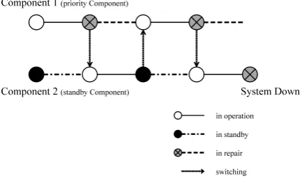
We consider the 2-component standby redundant system composed of Component 1 having priority and Component 2 which is a standby component. In this case, the component with priority means a component which is always used when-ever it is available. In contrast, the standby component means a component which stands by whenever the component with priority is available. When the priority component falls in failure, it starts to be repaired immediately and the standby component starts to operate. If the standby component falls in failure during repairing the priority component, the entire system becomes down. The outline of behavior in this system is illustrated in Figure 1. The solid line represents the operating status of each component. The dashed line represents the repair status of Component 1, the dashed-dotted line represents the standby status of Component 2. In addition, the dotted arrowhead connecting Component 1 and Component 2 represents the switching of components.
Component 1 (priority Component)
[image:2.595.319.536.64.197.2]Component 2 (standby Component) System Down in operation in standby in repair switching
Fig. 1. 2-component standby redundant system with priority
Initially, at time t = 0, Component 1 is working, and Component 2 is in the standby state. At this time, the standby time of the Component 2 is not included in its lifetime. When Component 1 fails, it starts to be repaired immediately and then Component 2 starts to work. If the repair of Component 1 has been completed and Component 2 is still working, then Component 1 starts to work immediately, and Component 2 is in a standby state. However, if Component 2 fails during the repair of Component 1, the entire system goes down. The switching of components is reliably executed, and it is assumed that the switchover time is instantaneous.
III. OUTCOME OF PREVIOUS LITERATURE
For the 2-component standby redundant system of Figure 1, Buzacott [6] has derived MTTF under the situation that the failure and repair time distributions of each component are explicitly prescribed as individual specific probability distributions On the other hand, under the situation that Component 2 has an exponential failure time distribution, Osaki [7], [8] has derived MTTF of the 2-component standby redundant system of Figure 1. All the distribution functions of the failure and repair times in each component have to be explicitly specified for evaluating MTTF by using the theoretical formulae by Osaki and Buzacott.
However, in some practical situations, it is difficult to know exactly the probability distributions of failure and repair times. On the other hand, in most practical cases, the mean and variance about failure and repair times in respective components will be at least known based on historical information.
In recent years, Takemoto and Arizono [9] and Oigawa et al. [10] have respectively considered the evaluations of mean time to failure and variance of failure time in the 2-component standby redundant system illustrated in Figure 1. In these evaluations, the followings have been assumed:
i) The failure time distribution of Component 1 has the cumulative distribution function (CDF)F1(t)with mean EF1 = 1/λ1 and variance VF1.
ii) The repair time of Component 1 obeys the probability distributionG1with mean EG1 and varianceVG1.
iii) The failure time of Component 2 obeys the probability distributionF2with mean EF2 and varianceVF2.
transformed into a mixed Erlang distribution under the con-straints of mean EG1 (or EF2) and varianceVG1 (or VF2).
Then, the system has been reconstructed by four types of tentative systems based on the combinations of respective Erlang distributions in the mixed Erlang distributions for the repair time distribution of Component 1 and the failure time distribution of Component 2. The respective tentative systems have been analyzed using Markov process theory because the state transition in the respective tentative systems can be expressed by a state transition diagram based on an exponential distribution. MTTFs in the respective tentative systems are weightedly summed up using the ratios of mixture on the mixed Erlang distribution.
As a consequence, Takemoto and Arizono [9] have defined MTTF of the entire system as follows:
M T T F =p1p2M T T F(n1,n2)
+ (1−p1)p2M T T F(n1+1,n2)
+p1(1−p2)M T T F(n1,n2+1)
+ (1−p1)(1−p2)M T T F(n1+1,n2+1)≡µ, (1)
where
M T T F(n1,n2)= ˜R(n1,n2)(0)
= 1/λ1 1−˜bn1(0)
n∑2−1
j=0
˜
dj(n1)(0) +
˜
a(0) 1−˜bn1(0) ×
n∑1−1
i=0 n∑2−1
j=0 n2∑−1−j
k=0
(
i+k k
)
˜bi(0)˜ck(0) ˜d
j(n1)(0), (2)
1
ni+ 1
< φ2i ≤ 1 ni
, (3)
pi =
(ni+ 1)φ2i −
√
(ni+ 1)(1−niφ2i)
φ2i + 1 , (4)
φ1=
√
VG1/EG1, (5)
φ2=√VF2/EF2, (6)
µ1= n1+ 1−p1
EG1
, (7)
λ2=
n2+ 1−p2 EF2
, (8)
˜
R(n1,n2)(s) = ˜u(n1)(s)
n∑2−1
i=0
˜
di(n1)(s)
+ ˜a(s)˜v(n1)(s)
n∑1−1
i=0 n∑2−1
j=0 n2∑−1−j
k=0
(
i+k k
)
טbi
(s)˜ck(s) ˜dj(n1)(s), (9)
˜
a(s) = 1
s+µ1+λ2, (10)
˜
b(s) = µ1
s+µ1+λ2, (11)
˜
c(s) = λ2
s+µ1+λ2, (12)
˜
d0(n1)(s) = 1, (13)
˜
dj(n1)(s) = ˜w(n1)(s) ×
j−1
∑
k=0
(
n1−1 +j−k j−k
)
˜
cj−k(s) ˜dk(n1)(s), (14)
˜
u(n1)(s) =
˜
R1(s)
1− {1−sR1˜ (s)}˜bn1(s)
, (15)
˜
v(n1)(s) =
1−sR1˜ (s) 1− {1−sR˜1(s)}˜bn1(s)
, (16)
˜
w(n1)(s) =
{1−sR1˜ (s)}˜bn1(s)
1− {1−sR˜1(s)}˜bn1(s)
. (17)
The notations of M T T F(n1,n2), M T T F(n1+1,n2),
M T T F(n1,n2+1) and M T T F(n1+1,n2+1) in equation
(1) denote the mean time to failure in the respective tentative systems. Further, the symbols ofpi,φ1,φ2,µ1and λ2 denote the parameters in the case of approximating the repair time distribution of Component 1 and the failure time distribution of Component 2 to the respective mixed Erlang distributions. In addition, the notations ofR˜(n1,n2)(s),˜a(s),
˜b(s), ˜c(s), d˜
j(n1)(s), u˜(n1)(s), v˜(n1)(s) andu˜(n1)(s) mean
the functions derived by Takemoto and Arizono [9] for evaluating MTTF in the 2-component standby redundant system. Further,R1(t) = 1−F1(t)and then,R1˜ (s)denotes the Laplace transformation forR1(t).
Further, Oigawa et al. [10] have addressed the derivation of the variance of the failure time of the considered 2-component standby redundant system with priority. Denote the probability density function (PDF) of the failure time distribution of the entire system byf(t). Then, the Laplace transformation forf(t)is defined as:
˜
f(s) =
∫ ∞
0
e−stf(t)dt. (18) On the other hand, since the reliability functionR(t)of the entire system is expressed as
R(t) = 1−
∫ t
0
f(τ)dτ, (19) the relationship between the Laplace transformations f˜(s)
and R˜(s) can be given as f˜(s) = 1−sR˜(s). Then, by applying the final-value theorem and the L’Hopital’s rule to the differential calculus forms for this relationship, the following equations can be shown:
d ds
˜
f(s)|s=0≡f˜(1)(0) =−E[t] =−µ, (20)
d2
ds2f˜(s)|s=0≡f˜ (2)
Therefore, the varianceV[t]of the failure time of the con-sidered 2-component standby redundant system with priority can be obtained as
V[t] = ˜f(2)(0)−
{
˜
f(1)(0)
}2
≡σ2, (22)
where
˜
f(2)(0) =p1p2f˜((2)n
1,n2)(0)
+ (1−p1)p2f˜((2)n
1+1,n2)(0)
+p1(1−p2) ˜f((2)n
1,n2+1)(0)
+ (1−p1)(1−p2) ˜f((2)n
1+1,n2+1)(0), (23)
˜
f((2)n
1,n2)(0) = −2˜u
(1) (n1)(0)
n∑2−1
j=0
˜
dj(n1)(0)
−2˜u(n1)(0)
n∑2−1
j=0
˜
d(1)j(n
1)(0)
+ 2˜a(0)˜v(n1)(0)
n∑1−1
i=0 n∑2−1
j=0 n2∑−1−j
k=0
(
i+k k
)
טbi(0)˜ck(0)
{
˜
dj(n1)(0)˜a(0)
(
1 +i+k
+h(n1,n2)(0)
˜
a(0)
)
−d˜(1) j(n1)(0)
}
, (24)
˜
u(1)(n
1)(0) =−
VF1+
(
1 λ1
)2
2
{
1−˜bn1(0)
}
−
1 λ1
˜bn1(0)
{
n1a˜(0) + λ1
1
}
{
1−˜bn1(0)
}2 , (25)
˜
d(1)j(n
1)(0) = ˜w
(1) (n1)(0)
j−1
∑
k=0
(
n1−1 +j−k j−k
)
טcj−k(0) ˜dk(n1)(0) −w˜(n1)(0)
j−1
∑
k=0
(
n1−1 +j−k j−k
)
×(j−k)˜a(0)˜cj−k(0) ˜dk(n1)(0)
+ ˜w(n1)(0)
j−1
∑
k=0
(
n1−1 +j−k j−k
)
טcj−k(0) ˜d(1)k(n
1)(0), (26)
˜
wn(1)1(0) =−v˜n1(0)h(n1,n2)(0)˜b
n1(0)
−n1a˜(0)˜bn1(0)˜vn1(0), (27)
h(n1,n2)(0) = ˜R(n1,n2)(0)
+
˜bn1(0) ˜R
(n1,n2)(0) +n1˜a(0)˜b
n1(0)
1−˜bn1(0)
, (28)
where note that the notations of f˜((ni)
1,n2)(0), u˜
(1) (n1)(0),
˜
d(1)j(n
1)(0)andw˜
(1)
n1(0)are similar to the notation of f˜
(i)(0).
Through the similar way,f˜((2)n
1+1,n2)(0),
˜
f((2)n
1,n2+1)(0)and
˜
f((2)n
1+1,n2+1)(0) can be obtained. Remind that the concrete
mathematical expressions of f˜((2)n
1+1,n2)(0),
˜
f((2)n
1,n2+1)(0)
andf˜((2)n
1+1,n2+1)(0)are omitted for convenience of the
num-ber of the paper.
IV. DERIVATION OF RELIABILITY FUNCTION In this study, based onµandσ2 derived as equations (1) and (22), we evaluate the probability density functionf(t)
of the failure time of the entire system. As for derivation of µ and σ2, we have considered that only the mean and variance of failure and repair times in each component are given as the limited information. In other words, the basic condition in this study is that the distribution of failure and repair times in each component is unknown and not specified. Hence, we do not suppose a specific distribution type to evaluate the probability density function f(t)of the failure time in the entire system. Then, it is widely known that the maximum entropy principle brings an elegant solution for deriving the probability density function under the constraints of the values of moments. Therefore, we apply the maximum entropy principle to obtain the probability density function f(t)of the failure time in the entire system.
Based on the maximum entropy principle, the identifica-tion problem off(t)can be formulated as follows:
Maximize
f(t)
H(f) =−
∫ ∞
0
f(x) logf(x)dx, (29) subject to
∫ ∞
0
f(x)dx= 1, (30)
∫ ∞
0
xf(x)dx=µ, (31)
∫ ∞
0
(x−µ)2f(x)dx=σ2. (32) By using equations (29)–(32), a Lagrange function is defined with introducing Lagrange multipliersα1,α2 andα3 as
V =H(f)−α1
{∫ ∞
0
f(x)dx−1
}
−α2
{∫ ∞
0
xf(x)dx−µ
}
−α3
{∫ ∞
0
(x−µ)2f(x)dx−σ2
}
. (33)
Through adopting the variational method to the Lagrange functionV, we have
δV
δf = −
{
logf(x) + 1
}
−α1−α2x−α3(x−µ)2= 0. (34) From equation (34),f(x)is expressed as
f(x) =e−1−α1e−α2xe−α3(x−µ)2. (35)
At the same instant, by partially differentiatingV withα1, α2 and α3, we have equations (30)–(32). Therefore, based on equations (30)–(32) and (35),f(x)is rewritten as
where
C=e−1−α1−α3µ2eα3
(2µα
3−α2 2α3
)2
, (37)
m= 2µα3−α2
2α3 , (38) δ2= 1
2α3. (39) Accordingly, the derivation of f(x) becomes a problem of finding C,m andδ2.
Furthermore, by substituting equation (36) for equation (30), (31) and (32), the following equations can be shown:
C
∫ ∞
0
e−(x−2δm2)2dx= 1, (40)
C
∫ ∞
0
xe−(x−2δm2)2dx=µ, (41)
C
∫ ∞
0
(x−µ)2e−(x−2δm2)2dx=σ2. (42)
Then, from equations (40), we can derive as follows:
1
C =
∫ ∞
0
e−(x−2δm2)2dx. (43)
Moreover, by multiplying both sides of equation (43) by
1/√2πδ2, we obtain the following equation:
1
√
2πδ2
1
C =
1
√
2πδ2
∫ m
0
e−(x−2δm2)2dx
+√1 2πδ2
∫ ∞
m
e−(x−2δm2)2dx. (44)
The right side means the upper side probability function of the normal distribution with mean m and variance δ2. Through the variable transformation of t = (x−m)/δ, equation (44) is converted to
1
√
2πδ2
1
C =
1
√
2π
∫ 0
−m δ
e−t
2
2dt+1
2. (45)
Further, by replacing t by√2τ, equation (45) is expressed as
1
√
2πδ
1
C =
1 2 +
1
√
π
∫ 0
−√m
2δ e−τ2dτ
=1 2 −
1 2
(
2
√
π
∫ −√m
2δ
0
e−τ2dτ
)
=1 2 −
1 2erf
(
−√m
2δ
)
. (46)
Then, the functionerf(z)is known as the error function as follows:
erf(z) = √2
π
∫ z
0
e−t2dt. (47)
The error function is frequently used in probability theory, statistics, material science, and partial differential equation. Further, the error function and confluent hypergeometric function have the following relationship:
erf(x) = √2x
π1F1
(
1 2;
3 2;−x
2
)
. (48)
Note that the confluent hypergeometric function is classified as special functions. Then, the confluent hypergeometric function is defined as
1F1(β;γ;z) = Γ(γ) Γ(β)
∞
∑
n=0
Γ(β+n) Γ(γ+n)
zn
n!. (49)
Furthermore, the following Kummer transformation can be applied to be confluent hypergeometric function:
1F1(β;γ;z) =e−z1F1(γ−β;γ;−z). (50) Consequently, based on equation (48) and (50), equation (46) is transformed as follows
C=√ 1
πδ2
2 +me −m2
2δ2
1F1
(
1;3 2;
m2
2δ2
). (51)
Further, as for equations (41) and (42), we have respectively the following equations:
C= µ−m
δ2e−2mδ22
, (52)
C=µ
2+σ2−m2−δ2 mδ2e−m2δ22
. (53)
Then, based on equations (52) and (53), the following equations can be shown:
δ2=−µm+µ2+σ2. (54) Accordingly, by substituting equation (54) for equation (51) and (52) (or (53)), we can obtain the following function for m:
(µ−m)
{√
π(−µm+µ2+σ2)
2 +me
− m2
2(−µm+µ2 +σ2 )
×1F1
(
1,3
2;
m2
2(−µm+µ2+σ2)
)}
−(−µm+µ2+σ2)e− m
2
2(−µm+µ2 +σ2 ) = 0. (55)
It is difficult to solve analytically equation (55) for m because that equation (55) contains the confluent hyperge-ometric function. However, we can derive the value of m satisfying equation (55) numerically by appropriate search algorithms such as linear search. It is clear that we can get the values of δ2 andC by calculated m. Moreover, by substituting equation (36) for equation (19), we can derive as follows.
R(t) = C
{√
πδ2
2 −(t−m)
×e−(t−2δm2)21F1
(
1;3 2;
(t−m)2 2δ2
) }
. (56)
V. NUMERICALANALYSIS
In this section, we investigate the validity of our proposal on evaluating the reliability function with the following procedures:
i) The mean and variance of failure and repair time in Component 1 are respectively given. Further, the mean and variance of failure time in Component 2 are also given.
ii) The probability distributions for the failure and repair time in Component 1 and the probability distribution for the failure time in Component 2 are individually specified as a particular probability distribution. iii) Through a million times of trials iterated in the Monte
Carlo simulation under the combination of specified probability distributions, the reliability in the entire system on timet is estimated.
iv) The proposed reliability function is compared with the reliability estimated through the Monte Carlo simula-tion.
As an example, suppose that EF1 = 1/λ1 = 100.0,
VF1 = 20.0
2, E
G1 = 5.0, VG1 = 1.5
2, E
F2 = 50.0,
and VF2 = 22.5
2, respectively. Moreover, the failure and repair time distributions in both components are respectively defined as the log-normal and/or Weibull distributions. The log-normal distribution and Weibull distribution are well known in the reliability field.
Based on the above numerical values and the supposition for the failure and repair time distributions, the values of µ andσ2for the failure times in the entire system are calculated as the following numerical value:
(
µ, σ2)= (1106.089,239852.167). Further, m,δ2 andC are obtained as follows:
(
m, δ2, C)= (1057.804,345871,144,0.000704). So, we can evaluate the reliability function in equation (56) by applying the above values of (m, δ2, C).
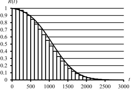
One of the results of comparing the simulation and the proposed reliability is shown in Figure 2. In Figure 2, the failure time distributionF1(t)and the repair time distribution G1(t) in Component 1 and the failure time distribution F2(t) in Component 2 are respectively supposed as the Weibull distribution with mean EF1 and variance VF1, the
log-normal distribution with mean EG1 and variance VG1
and the Weibull distribution with mean EF2 and variance
VF2.
From Figure 2, it has been confirmed that the shape of the reliability function proposed in this study resembles that of simulation result. Moreover, remark that similar results have been obtained under different conditions. Consequently, it has been confirmed that the proposed reliability function based on the maximum entropy principle is useful as an approximation method for the reliability evaluation under the condition that only the mean and variance of failure time in the entire system can be used.
0 0.1 0.2 0.3 0.4 0.5 0.6 0.7 0.8 0.91
[image:6.595.321.533.41.187.2]0 500 1000 1500 2000 2500 3000t
Fig. 2. Comparison of reliability based on proposed reliability function and the simulation results
VI. CONCLUSION
In this study, we have addressed the evaluation method of the reliability function in the 2-component standby redundant system with priority. Then, by utilizing the evaluation results for the mean time to failure by Takemoto and Arizono [9] and the variance of the failure time by Oigawa et al. [10], we have succeeded in deriving the evaluation method of the reliability function in the 2-component standby redundant system with priority. In concrete, by using only the mean and variance of the failure time in the entire system, the reliability function in the 2-component standby redundant system with priority has been derived based on the maximum entropy principle.
Then, it would like to be the future issue to establish the way of the optimal preventive maintenance of the system by using the reliability indices such as the reliability function.
REFERENCES
[1] I. Gersbakh,Reliability Theory with Applications to Preventive Main-tenance, Springer-Verlag, 2000.
[2] A. Birolini, Reliability Engineering: Theory and Practice (6th ed.), Springer-Verlag, 2010.
[3] Y. L. Zhang, G. J. Wang, “A Deteriorating Cold Standby Repairable System with Priority in Use,”European Journal of Operation Research, Vol. 183, No. 1, pp. 278–295, 2007.
[4] L. Yuan, X. X. Meng, “Reliability Analysis of a Warm Standby Re-pairable System with Priority in Use,”Applied Mathematical Modeling, Vol. 35, No. 9, 4296–4303, 2011
[5] K. N. F. Leung, Y. L. Zhang, K. K. Lai, “Analysis for a Two-dissimilar-component Cold Standby Repairable System with Repair Priority,”
Reliability Engineering & System Safety, Vol. 96, No. 11, pp. 1542– 1551, (2011).
[6] J. A. Buzacott, “Availability of Priority Standby Redundant Systems,”
IEEE Transactions on Reliability, Vol. R-20, No. 2, pp. 60–63 (1971). [7] S. Osaki, “Reliability Analysis of a Two-unit Standby Redundant System with Priority,”Canadian Journal of Operations Research, Vol. 8, No. 1, pp. 60–62 (1970).
[8] S. Osaki,Stochastic Models in Reliability and Maintenance, New York, Springer, 2002.
[9] Y. Takemoto, I. Arizono, “A Study of MTTF in Two-unit Standby Redundant System with Priority under Limited Information about Failure and Repair Times,”Journal of Risk and Reliability, Vol. 230, No. 1, pp. 67–74 (2016).