Average Error Rates and Achievable Capacity in Large Office Indoor Wireless Environments

IEEE Proof

Average Error Rates and Achievable Capacity in

Large Office Indoor Wireless Environments

Indrakshi Dey, Member, IEEE, Geoffrey G. Messier, Member, IEEE, and Sebastian Magierowski, Member, IEEE

Abstract— Performance of common digital modulation

tech-1

niques is analyzed over indoor wireless environments modeled 2

through the recently proposed joint fading and two-path shadow-3

ing (JFTS) channel model. Mathematically tractable expressions 4

for the instantaneous signal-to-noise ratio statistics, average bit 5

error rates, and achievable channel cutoff rates are derived. 6

Analytical results are used to: 1) investigate the impact of differ-7

ent JFTS model parameters and different modulation techniques 8

on bit error rates and cutoff rates and 2) demonstrate how the 9

JFTS channel model affects system performance in comparison 10

with conventional empirical channel models. Finally simulation 11

results are used to corroborate this analysis and evaluate the 12

usefulness of such an analysis. 13

Index Terms— JFTS, ABER, M-QAM, M-PSK.

14

I. INTRODUCTION

15

A. Motivation

16

T

HE wide variety of applications of indoor wireless com-17

munication has resulted in the increased demand of exact 18

theoretical analysis of high capacity wireless communication 19

systems when implemented on indoor wireless access points. 20

For example, expressions for the average bit error rate (ABER) 21

are essential for designing effective signaling and error control 22

coding schemes, as they provide insights into how system 23

parameters affect performance and are more computationally 24

efficient for analyzing system performance. 25

It is well-known that indoor wireless links are affected by 26

both small scale fading and shadowing effects. Therefore, 27

it will be more accurate to account for the combined small 28

and large scale channel effects while evaluating system per-29

formance. Common composite channel models [1], [2], [3] 30

that combine large and small scale channel effects have been 31

developed primarily for outdoor channels, where the users are 32

highly mobile transiting through several scattering clusters. 33

As a result, a range of main waves arrive at the mobile, the 34

strength of each of which can be drawn from the log-normal 35

or the Gamma distribution. 36

In an indoor wireless environment, the path between the 37

access point and the users is too short for shadowing to be 38

Manuscript received December 21, 2016; revised April 30, 2017 and June 18, 2017; accepted July 12, 2017. The associate editor coordinating the review of this paper and approving it for publication was J. Choi.

(Corresponding author: Indrakshi Dey.)

I. Dey and G. G. Messier are with the Department of Electrical and Computer Engineering, University of Calgary, Calgary, AB T2N 1N4, Canada (e-mail: [email protected]; [email protected]).

S. Magierowski is with the Department of Electrical Engineering and Computer Science, Lassonde School of Engineering, York University, Toronto, ON M3J 1P3, Canada (e-mail: [email protected]).

Digital Object Identifier 10.1109/TCOMM.2017.2729552

accurately characterized by the log-normal distribution and the 39 mobile users restrict their movement within a small area due to 40 the incapability of most WLAN standards to handle hand-offs 41 efficiently. A new composite channel model, called the joint 42 fading and two-path shadowing (JFTS) model, is proposed 43 in [4]. Based on an extensive channel measurement campaign, 44 the JFTS model is shown to be a more accurate model for 45 characterizing indoor WLAN channels. 46 The JFTS distribution has also some added advantages over 47 other common composite channel models. Since the JFTS 48 distribution is a general model that includes a wide variety 49 of channel conditions as special cases (no fading, no shadow- 50 ing, deep fading, heavy shadowing, etc.), the expressions for 51 different performance metrics evaluated over the JFTS channel 52 will provide us with the achievable performance measures over 53 a large variety of practical channel conditions. 54 The JFTS distribution is fundamentally different from 55 other composite fading/shadowing models. It is a convolu- 56 tion of the Ricean fading and the two-wave with diffused 57 power (TWDP) shadowing models [5]. It follows the bivariate 58 non-centralized chi-squared distribution and therefore, cannot 59 approach Gaussian statistics. This is unlike conventional fad- 60 ing models that can approach zero-mean complex Gaussian 61 statistics under different propagation conditions. This suggests 62 that performance of different communication systems over 63 the JFTS channel will be very different than what has been 64 predicted by conventional fading/shadowing models and moti- 65 vates the need for analytical error rate and achievable capacity 66 expressions specifically for the JFTS channel. 67 The work in [4] is extended in [6] and [7] by deriving 68 expressions for the first-order statistics and Cumulative Distri- 69 bution Function (CDF) of the JFTS distribution respectively. 70 In [8], expressions for ergodic capacity achievable by different 71 adaptive transmission techniques over a JFTS channel are 72 derived. The effect of these adaptive schemes on the rela- 73 tionship between optimal cutoff signal-to-noise ratio (SNR) 74 and the average received SNR for JFTS faded/shadowed links 75 is also studied in [8]. However, to the best of the authors’ 76 knowledge, a detailed study on how different M-ary coherent 77 and noncoherent modulation techniques perform when applied 78 to a JFTS faded/shadowed link has not yet been conducted in 79

literature. 80

B. Main Results and Paper Organization 81

The main contributions of the paper are summarized as 82

follows. 83

IEEE Proof

• We derive analytically tractable expressions for ABER 84

of coherent and noncoherent binary, and coherent 85

M-ary modulation techniques over a non-Gaussian indoor

86

WLAN environment, which can be accurately charac-87

terized by the JFTS model. We focus on the CDF 88

based approach [9] for deriving ABER expressions. 89

We also study the impact of different JFTS distribu-90

tion parameters on the performance based on numerical 91

results. 92

• In this paper, we provide expressions that are numeri-93

cally efficient and simple to handle. Towards this end, 94

we derive error rate expressions that involve truncation 95

of the infinite series of the original expressions. The 96

approximate expressions are derived in a way such that 97

they guarantee that the area under the probability density 98

function (PDF) of the instantaneous SNR remains equal 99

to 1. However, the truncation bound is decided based on 100

the study done in [10] for analysis of bandwidth efficiency 101

for the JFTS channel. 102

• We also evaluate the channel cutoff rate associated with 103

M-ary signaling and JFTS channels both in presence

104

and absence of channel magnitude and phase estimates. 105

The channel cutoff rate R0 of the communication link is

106

defined as a channel capacity related quantity such that 107

for any Rc < R0, it is possible to construct a channel

108

code using block length n and coding rate Rc capable of

109

maintaining an average error probability less than or equal 110

to 2−n(R0−Rc)_{[11]. Quantifying the channel cutoff rate is}

111

done using the Chernoff bound calculation. Therefore, 112

the channel cutoff rate obtained in this way can also be 113

used as an analytical bound limiting the bit error perfor 114

M-ary signaling techniques are implemented.

115

The paper is organized as follows. Section II describes 116

the statistics of instantaneous received SNR over a JFTS 117

faded/shadowed channel. The error performance and chan-118

nel capacity analyses are presented in Section III and 119

Section IV. Numerical results and discussions are given 120

in Section V, while concluding remarks are provided in 121

Section VI. 122

II. STATISTICS OFINSTANTANEOUSSNR

123

Let s(k)represent the transmitted data symbol with symbol 124

energy Es =E{|s(k)|2}that is transmitted over a composite

125

slow shadowed and flat faded wireless communication channel 126

with JFTS statistics. The bit energy is then defined as Eb=

127

Es/log2M, where M is the modulation constellation size used

128

for data transmission. The received data symbol y(k)over the 129

sampling instant k can be given by 130

y(k)=z(k)ejφ(k)s(k)+n(k) (1) 131

where n(k) is the complex Additive White Gaussian 132

Noise (AWGN) with one side power spectral density of N0,

133

φ(k)is the instantaneous phase and z(k)denotes the composite 134

fading/shadowing envelope which is JFTS distributed. 135

The first order statistics of the channel joint fading/ 136

shadowing stochastic process, z(k), can be represented by the 137

random variable, Z , which has a PDF given by [4] 138

fZ(z)=

4

i=1

m

h=1 biz Rh

2P1P2 e−

K−Sh− z2

2P2r2h 139

×

C1iI0

2z

K Sh(1−Ti)

P1P2

140

+C2iI0

2z

K Sh(1+Ti)

P1P2

(2) 141

and a CDF given by [7] 142

FZ(z)=

4

i=1

m

h=1

biRhrhe−K−Sh

2P1 √

P2 143

×

C1i Q1

K Sh(1−Ti)rh

P1 ,z

144

+C2i Q1

K Sh(1+Ti)rh

P1 ,z

(3) 145

where C1i = eShTi, C2i = e−ShTi, Ti =cos((i −1)π/7), 146

I0 is the 0th-order modified Bessel function of the first kind, 147

m is the quadrature order, Rh = _|w_rhh_|er

2

h−rh2/2 P1_, w

h are the 148 Gauss-Hermite quadrature weight factors [12], rhare the roots 149 of the Hermite polynomial for h = 1,2, . . . ,m, Q1 is the 150 Marcum Q-function and bi = aiI0(1) with a1 = ₁₇₂₈₀751 , 151

a2 = ₁₇₂₈₀3577, a3 = ₆₄₀49 and a4 = ₁₇₂₈₀2989. The behavior of 152 the JFTS distribution is guided by the fading parameter K , 153 shadowing parameter Sh, shape parameterand mean-squares 154 of the diffused and the shadowed components, P1 and P2, 155 respectively. For our analysis we have chosen the quadrature 156

order m=20. 157

If the instantaneous received SNR per symbol is defined as 158 γ (k)=z2_(k)E

s/N0 and the average received SNR asγ (k)= 159 E{z2_(k)}E

s/N0, where Es is the energy per symbol and N0 160 is the noise density (the noise power present in 1 Hz), the 161 PDF ofγ (for the sake of simplicity of notation, we drop the 162 sampling index k from here on) can be obtained in terms of 163 γ [13] by change of variables as 164

fγ(γ )= 4

i=1

m

h=1 biRh

γP1P2e

−K−Sh− γ

2γP2r2h 165

×

C1iI0

2

K Sh(1−Ti)γ

γP1P2

166

+C2iI0

2

K Sh(1+Ti)γ

γP1P2

(4) 167

whereis the mean-squared value of the JFTS envelope given 168 by =4P1P2(1+K)(1+Sh)[6]. The corresponding CDF 169 of γ can be defined as F_γ(γ ) = _−∞γ f_γ(u)du and can be 170 expressed as F_γ(γ )=Fz γE{Z2}/γ

. 171

IEEE Proof

expansion of modified Bessel function, I0(f)=∞_t=0(f/2)

2t

(t!)2 ,

176

we arrive at an alternative expression for (4) as 177

fγ(γ )= 4

i=1

m

h=1

∞

t=0 Ai,h

γ (t!)2e−

Bhγ /γ

178

×C1i C3iγ /γt+C2i C4iγ /γt (5) 179

where Ai,h = bi_PRh_1P2e−K−Sh, Bh = _{2 P}

2r_h2, C3i = K Sh(1−

180

Ti)/(P1P2) and C4i = K Sh(1 +Ti)/(P1P2). If we

181

truncate the infinite series summation to tmax, we can obtain

182

an approximate version of (5) as below, 183

f_γ(γ )≈ 4

i=1

m

h=1

tmax

t=0 Ai,h

γ (t!)2e

−Bhγ /γ

184

×D1tC1i C3iγ /γt+D2tC2i C4iγ /γt (6) 185

where D1t = γ (t!)

2

Ai_,h

γ

C3i

tt_max+1

u₌1 (u −1)! Bhγ u

and D2t =

186 γ (t!)2

Ai,h

γ

C4i

ttmax+1

u=1 (u −1)! Bγh u

for γ > 0 and Bh > 0.

187

The constants, D1t and D2t in (6) are derived for the sake

188

of guaranteeing that the area under the PDF of γ remains 189

equal to 1. For our numerical analysis, we have chosen tmax=

190

25 based on the observations in [10]. 191

Proposition 1: The exact and approximate expressions for

192

F_γ(γ )can be given by 193

F_γ(γ )=1−

4

i=1

m

h=1

∞

t=0

Ai,h(t+1,Bhγ /γ )

(t!)2_Bt+1

h

194

×

C1iC_3it +C2iC_4it

195

≈1−

4

i=1

m

h=1

tmax

t=0

Ai,h(t+1,Bhγ /γ )

(t!)2_Bt+1

h

196

×

D1tC1iC_3it +D2tC2iC_4it

(7) 197

where (·,·) is the generalized upper incomplete Gamma 198

function [12]. 199

Proof: See Appendix A.

200

In the next section, we will be using the CDF-based 201

approach and therefore, (7) for deriving the ABER expres-202

sions for different modulation techniques over a JFTS 203

faded/shadowed communication channel. 204

III. ERRORPERFORMANCEANALYSIS

205

In order to obtain the ABER of a large variety of modulation 206

techniques, the CDF-based approach of [9] and [14] will be 207

used in this section. 208

A. Binary Modulation Schemes

209

For any binary coherent and noncoherent modulation 210

technique, the ABER over a composite flat faded and slow 211

shadowed wireless communication channel suffering from 212

AWGN can be expressed in terms of the CDF of the instan-213

taneous SNR as [9] 214

P_bBinary(e)= α β

2(β)

_∞

0 γ

β−1 _e−αγ _F

γ(γ )dγ (8) 215

where α = 1 for Binary Phase Shift Keying (BPSK) and 216 α = 1/2 for Binary Frequency Shift Keying (BFSK). If the 217 modulation is differential or noncoherent, β = 1, while for 218 coherent modulation,β=1/2. 219

Proposition 2: The ABER expression for any coherent 220 or noncoherent binary modulation technique over a JFTS 221 faded/shadowed channel can be obtained in exact and approx- 222 imate mathematically tractable format as 223

P_bBinary(e) 224

= 1

2 −

4

i=1

m

h=1

∞

t=0 Ai,h

(t!)2

C1iC_3it +C2iC_4it

225

× αβγβ

2β(β)

(β+t+1) (αγ +Bh)β+t+1

226

×2F1

1, β+t+1;β+1; αγ αγ +Bh

227

≈ 1

2 −

4

i=1

m

h=1

tmax

t=0 Ai,h

(t!)2

D1tC1iC_3it +D2tC2iC_4it

228

× αβγβ

2β(β)

(β+t+1) (αγ +Bh)β+t+1

229

×2F1

1, β+t+1;β+1; αγ αγ +Bh

. (9) 230

wherepFq(·)is the generalized hyper-geometric function [12] 231 and p,q are integers. 232

Proof: See Appendix B. 233

B. M-Ary Coherent Modulation Schemes 234

In order to evaluate the error performance of M-ary coherent 235 modulation techniques over a composite fading/shadowing 236 channel, we need to calculate an integral of the form [9] 237

P_bM-ary(e,g)= √1

2π _∞ 0 F_γ v2 g

e−v2/2dv (10) 238 where g depends on the modulation type [13]. 239

Proposition 3: For a JFTS channel, ABER expression for 240 coherent M-ary modulation technique can be obtained in exact 241 and approximate mathematically tractable format as 242

P_bM-ary(e,g) 243

= 1

2 −

4

i=1

m

h=1

∞

t=0 Ai,h

(t!)2

C1iC_3it +C2iC_4it

244

×2t+1 √

gγ (t+3/2) (gγ+2Bh)t+3/2

2F1

1,t+3

2; 3 2;

gγ gγ+2Bh

245

≈ 1

2 −

4

i=1

m

h=1

tmax

t=0

D1tC1iC_3it +D2tC2iC_4it

Ai,h

(t!)2 246

×2t+1 √

gγ (t+3/2) (gγ+2Bh)t+3/2

2F1

1,t+3

2; 3 2;

gγ gγ+2Bh

. 247

(11) 248

Proof: See Appendix C. 249

IEEE Proof

the product of the fading parameter K and the shadowing

252

parameter Sh. Hence, when K , Sh, or both increases, the

253

ABER performance improves. It can also be concluded that 254

ABER is also influenced by the-parameter. However, exactly 255

how much ABER is affected by a change in is difficult 256

to predict strictly by inspecting the ABER expressions. The 257

sensitivity to changes inis best evaluated using the ABER 258

plots presented in Section V. 259

1) M-Ary Quadrature Amplitude Modulation (M-QAM):

260

Using unified approximation, as is done in [13], the ABER 261

expression of general order M-QAM modulation over a com-262

posite fading / shadowing channel is given by [9] 263

P_bM-QAM(e)∼= 4

log2M

1−√1

M

√M/2

n=1

P_bM-ary(e,gn−Q)

264

(12) 265

where gn−Q = 3(2n − 1)2log2M/(M − 1). The ABER

266

expression for general order M-QAM over JFTS channel can 267

be expressed by substituting (11) in (12) and putting g=gn−Q

268

in (11). 269

2) M-Ary Phase Shift Keying (M-PSK): Using unified

270

approximation, as is done in [13], the ABER expression of 271

Gray-coded coherent M-PSK modulation over a composite 272

fading / shadowing channel is given by [9] 273

P_bM-PSK(e)∼= 2

max(log2M,2)

max(M/4,1)

n=1

P_bM-ary(e,gn−P)

274

(13) 275

where gn−P = 2(log2M)sin2((2n −1)π/M). The ABER

276

expression for coherent M-PSK over JFTS channel can be 277

expressed by substituting (11) in (13) and putting g =gn−P

278

in (11). 279

It is note-worthy that in this paper, we have shown 280

how the JFTS distribution provides mathematically tractable 281

error probability expressions in terms of generalized hyper-282

geometric functions. Such expressions can be obtained only 283

numerically for the commonly used Suzuki / Nakagami - log-284

normal distributions using log-normal approximations [15]. 285

However, this approximation is only valid for large log-286

normal spreading factor,σ. Easy-to-use expressions for ABER 287

of basic modulation techniques exist in literature only for 288

K-fading channels [3] among commonly used fading/ 289

shadowing channel models. Yet even for Gray-coded M-PSK, 290

symbol error probability over K-fading channel involves an 291

unsolvable integral which can only be evaluated numerically. 292

IV. ACHIEVABLECAPACITYANALYSIS

293

It has been argued in [16] that the average capacity measure 294

is only an upper bound on the channel capacity achievable 295

without transmitter feedbacks. Since for a JFTS channel, the 296

average capacity derived in [8] can only be expressed in terms 297

of infinite series summation, it is more appealing to obtain the 298

channel cutoff rate achievable using only variable rate M-ary 299

signaling. The channel cutoff rate can be calculated using [11] 300

R0=2log₂(M)−log₂

M

j₌1

M

l₌1

C(sˆj,sj)

(14) 301

whereC(sˆj,sj)is the Chernoff bound on the pairwise error 302 probability [13] associated with choosing the sequence sˆ = 303 (sˆ[1], . . . ,sˆ[L]) at the receiver when the sequence s = 304 (s[1], . . . ,s[L])is transmitted over the communication link. 305 The Chernoff bound can be calculated in presence of perfect 306 channel state information (CSI) as [18], [19] 307

CCSI(sˆj,sj)=EZ

e−z2|d j|

2 4

[bits/symbol] (15) 308

and in absence of any CSI as [18], [19] 309

CNCSI(sˆj,sj, λ)=e−λ

2_|dj|2

EZ

e−λz|dj|2

[bits/symbol] (16) 310

where|dj|2= |ˆsj−sj|2/N0, N0 is the noise spectral density 311 of the corrupting AWGN and λ is a nonnegative real valued 312 parameter over which (16) can achieve the tightest possible 313 exponential bound on the achievable cutoff rate in absence of 314

any CSI. 315

Proposition 4: For a JFTS channel, the Chernoff bound in 316 presence of perfect CSI is given by by putting (5) in (15) and 317 using integral solution from [17, p. 709, eq. (6.643.2)],1 318 CCSI(sˆj,sj) 319

= 4

i=1

m

h=1

biRhrh2e−K−Sh

P1(2+ |dj|2P2r_h2)

320

×

e

8K Sh(1−Ti)r2 h P1(4+|_{d j}|2 P2r2_h)

eShTi +_e−

ShTi+8K Sh(1+Ti)r2h P1(4+|_{d j}|2 P2r2_h)

(17) 321

and in absence of any CSI is given by 322 CNCSI(sˆj,sj) 323

= 4

i=1

m

h=1

biRhe−K−Sh

2P1P2

324

× π

0

(1−√πν1erfc(ν1)eν

2

1+ShTi)_dθ 325

+

_π

0

(1−√πν2erfc(ν2)eν

2

2−ShTi)_dθ

(18) 326

where ν1 = λd2_j

P2rh2

2₍1₊2 P2rh2) −

K Sh(1−Ti)

P1P2 cos(θ), ν2 = 327

λd2_j

P2rh2

2(1+2 P2r_h2) −

K Sh(1+Ti)

P1P2 cos(θ) and erfc(u) = 328

2

√_{π u}∞ e−γ2dγ is the complimentary error function. 329 In absence of CSI, minimizingλin (16) will maximize the 330 cutoff rate. Without side information, no uniform minimization 331 of λ exists [19]. In that case, (18) has to be evaluated 332 numerically using the Laguerre-Gauss Quadrature method and 333 substituted back in (17) to derive the expression for the 334 Chernoff factors of JFTS fading/shadowing link without any 335 CSI available at the receiver. 336

IEEE Proof

TABLE I

GENERALIZEDRANGE OFVALUES FOR THEPARAMETERS OFJFTS DISTRIBUTION

V. NUMERICALRESULTS ANDDISCUSSION

337

The derived mathematically tractable expressions for the 338

ABER of coherent / noncoherent binary modulation techniques 339

like BPSK, BFSK, general order M-QAM and coherently 340

detected M-PSK are numerically evaluated and plotted as 341

functions of the parameters of the communication channel 342

model and the modulation techniques. The analytical results 343

are compared with those obtained through Monte Carlo simu-344

lation in order to validate the proposed analysis. For plotting 345

the analytical results, we have chosen the approximation 346

index, m=20. 347

The wireless communication channel between the transmit-348

ter and the receiver is assumed to be suffering from AWGN 349

and the composite fading / shadowing envelope is assumed 350

to be JFTS distributed, where all the channel samples are 351

statistically independent. The channel samples are generated 352

using JFTS distributed random variables Z = X Y where

353

X are Ricean distributed and Y are TWDP distributed. All

354

the analytical and simulation results are evaluated for single 355

channel receivers and are averaged over 100 independent 356

random channel realizations. The ABER results are plotted 357

as functions of the average SNR per bit (Eb/N0) in decibels.

358

The behavior of the JFTS distribution is guided by its 359

fundamental parameters K , Sh and. The ranges of values

360

for those model parameters that are suitable for different 361

scenarios within the large office indoor wireless environments 362

are compiled in [4]. The particular set of JFTS parameters 363

that are used for numerical analysis and generating simulation 364

results in this paper are enlisted in Table I. 365

A. Error Probability Performance

366

1) Performance of Modulation Techniques: The first set of

367

curves in Fig. 1 are generated for evaluating performance of 368

different modulation techniques over a JFTS fading / shadow-369

ing communication channel. Both analytical and simulation 370

Fig. 1. Comparative simulation and analytical average bit error rate performances of coherent M-PSK and M-QAM over a JFTS faded / shadowed communication link.

Fig. 2. Average simulated bit error rate performances of 16-QAM over JFTS faded / shadowed communication link with (a) Sh= 6 dB,= 0.3 and (b) Sh =−4 dB,= 0.9.

results are plotted for each modulation scheme. All the results 371 are generated for a fixed set of JFTS parameters, K =6.5 dB, 372

Sh = 5 dB and = 0.8. This set of parameters are 373 encountered when the mobile WLAN user and the access point 374 are separated by 1 set of dry-wall or partition, as tabulated in 375 Table I. It is evident from Fig. 1 that the derived analytical 376 results from (9) and (11) offer a good agreement with that 377 of the simulation results and they fall within 1−2 dB of 378 the simulation results. It is to be noted that in many cases 379 analytical results do not exactly match the simulation results as 380 the analytical expressions involve the approximation index m. 381

[image:6.612.332.544.57.242.2] [image:6.612.59.291.58.242.2]

IEEE Proof

Fig. 3. Average bit error rate performances of 16-QAM over JFTS faded / shadowed communication link with (a) K = 6.5 dB, = 0.8 and (b) K=6 dB, Sh= −4 dB.

Simulation and analytical ABER performances are plotted 388

for 16-QAM. The performance of 16-QAM deteriorates as 389

the value of K decreases with fixed Sh and . This is due

390

to the fact that as K decreases, the power contributed by the 391

strong specular components decreases in comparison to that 392

contributed by the diffused and scattered components, resulting 393

in degradation of overall system performance. 394

The improvement in performance due to the increase in 395

K -factor from 2 dB to 5 dB or 5 dB to 8 dB is not

396

proportional to the improvement for increasing K from 8 dB 397

to 11 dB. This is due to the fact that for a JFTS channel, 398

the Sh andparameters also influence the channel behavior.

399

A high Sh factor corresponds to a low severity in shadowing.

400

A low represents a scenario where only one scattering 401

cluster dominates instead of two thereby also resulting in low 402

shadowing severity. Hence, with a high Shand lowcoupled

403

with high K -factors, the communication channel approaches 404

the “no fading” scenario. As a result changing the K -factor 405

from 8 dB to 11 dB does not cause any further improvement 406

in performance. 407

To emphasize the effect of Sh and , the ABER

perfor-408

mance of 16-QAM is plotted for only K =2 dB and 8 dB 409

in the second subplot of Fig. 2. In this case a low Sh factor

410

of−4 dB and a highfactor of 0.9 is used. This represents 411

a condition where the user and the access point are separated 412

by 2−3 partitions. The difference in performance due to the 413

increase in K -factor is completely obliterated for this set of 414

shadowing parameters. A low Shand a highcorresponds to

415

a very high severity in shadowing and further degrading fading 416

by a reduction in K does not further degrade performance in 417

any significant way. 418

Fig. 3(a), is generated by varying the Sh parameter of the

419

JFTS distribution with fixed K and at 6.5 dB and 0.8 420

respectively. This set of K and parameters represent a 421

scenario where the user and the access point are separated by 422

2−3 dry-walls or partitions. It is evident from Fig. 3(a) that 423

lowering the Sh-parameter value results in deteriorated system

424

performance. A larger Sh factor represents large variations

425

Fig. 4. Average bit error rate performances of 16-QAM over JFTS faded / shadowed communication link, where the curves are generated by varying all the JFTS parameters, K , Shandsimultaneously.

in the main wave amplitudes contributed by each scattering 426 neighborhood resulting in approximately equable number of 427 high and low, thereby reducing the overall severity of shad- 428 owing. On the other hand, a low Sh factor depicts a scenario 429 where each scattering cluster contributes a very small range of 430 discrete shadowing values, higher in magnitude and encoun- 431 tered repeatedly. This condition results in an increased severity 432 in shadowing, thereby degrading overall system performance. 433 The curves in Fig. 3(b) are generated by varying only the 434 -parameter of the JFTS distribution but keeping a fixed 435

K and Sh at 6 dB and −4 dB respectively. This set of 436

[image:7.612.64.288.57.255.2]

IEEE Proof

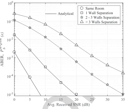
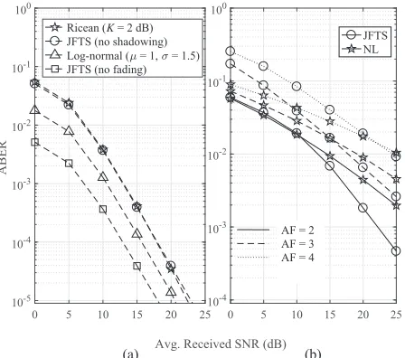
Fig. 5. Comparative average bit error rate of (a) QPSK over JFTS link with that over traditional channel models and (b) 16-QAM over a JFTS link with that over composite Nakagami - log-normal (NL) link.

is a result of the different small-scale fading and shadowing 464

statistics imposed by the JFTS model. 465

The average SNR per symbol requirement increases even 466

further by around 10 dB, if the user and the access point 467

is separated by 2 −3 sets of partitions (K = 6.5 dB, 468

Sh = −1.5 dB and = 0.25). This happens due to the

469

lack of strong specular components and the presence of at 470

least two scattering clusters between the transmitter and the 471

receiver, which jointly deteriorates the overall system perfor-472

mance. However, for propagation conditions that correspond 473

to an increase in the number of separations by more than 3 474

(i.e. K = 5.5 dB, Sh = −7.5 dB, = 0.15), the average

475

SNR per symbol requirement only increases by a maximum 476

of 5 dB, in order to achieve the same ABER performance. The 477

reason for this can be imparted to the low-factor, where the 478

effect of one scattering cluster is much stronger than the other 479

one. As a result, system performance is effectively affected 480

by only one scattering cluster, even in the presence of at least 481

two scattering clusters. 482

3) Comparison With Outdoor Channel Models: To

demon-483

strate how JFTS channel performance compares to con-484

ventional channel models, Fig. 5(a) is used to compare 485

performances of QPSK over JFTS, Ricean and log-normal 486

distributed communication channels. We have chosen the 487

Ricean distribution (K = 2 dB) to compare its impact on 488

performance with that of the JFTS channel with no shadowing 489

condition (K =2 dB, Sh=1000 dB,=0). The log-normal

490

distribution (μ=1,σ =1.5) is selected to compare with the 491

special case of JFTS channel with no fading (K =1000 dB, 492

Sh = −3 dB,=0.2). These particular set of JFTS

parame-493

ters is selected for comparison as they correspond to a TWDP 494

distribution with the same mean and standard deviation. The 495

performance over Ricean channel is almost equivalent to the 496

no shadowing JFTS case, as with=0, the JFTS distribution 497

reduces approximately to Ricean distribution. However, there 498

exists a small difference in performance owing to the minute 499

amount of shadowing still present in the JFTS channel with 500

Sh = 1000 dB. However, that is not the case with the 501 log-normal and the no fading JFTS channels. This is because, 502 putting a very high K in the JFTS distribution reduces it 503 approximately to the TWDP distribution accounting for max- 504 imum of two scattering clusters. The TWDP distribution is 505 very different from the log-normal distribution which accounts 506 for the transition through several local neighborhoods, each of 507 which consisting of different clusters of scattering objects. 508 To illustrate how the JFTS channel performance compares 509 to more conventional outdoor composite fading/shadowing 510 channel models, Fig. 5(b) is used to compare the performance 511 of 16-QAM over JFTS and Nakagami - log-normal (NL) 512 faded / shadowed communication channels. We have chosen 513 the NL distribution, as the Nakagami-m can be varied to model 514 a variety of fading distributions including the Rayleigh and the 515 Ricean distributions. The channel parameters are chosen so 516 that the JFTS and NL channels contribute the same amount 517 of fading (AF). As shown in [6], a JFTS distribution with 518

K =7 dB, Sh =6 dB and=0.7, contributes an AF of 2 519 which is same as that contributed by NL distribution with 520

m = 1 and σ =2.8 (4.4 dB). For these sets of parameters, 521 performance over a JFTS channel is worse than that over 522 a NL channel for SNRs less than 10 dB (γ ≤ 10 dB). 523 For higher SNRs per bit of around 10 dB and more, JFTS 524 offers a performance gain over NL. While only the simulation 525 results are shown for brevity, this same pattern in performance 526 repeats itself even for the set of JFTS (K = 5,2 dB, Sh = 527

−5,−10 dB, = 0.3,0.5) and NL (m = 1,1, μ = 1,1, 528 σ =3.6,4.2 (5.5, 6.2 dB)) parameters that contribute AFs of 529 3 and 4 respectively. This improvement in performance for the 530 JFTS distribution at higher SNRs occurs due to the fact that 531 for the JFTS distribution, there still exists a very small group 532 of specular components as long as K = 0. While, m = 1 533 for NL distribution represents a small scale fading condition, 534 which is equivalent to Rayleigh fading with the absence of 535 any specular component. 536 In addition, in order to visualize the difference between 537 JFTS and NL distributions, Fig. 6 exhibits their PDFs. The 538 model parameters for both the distributions are selected such 539 that they contribute the same amount of AF. The PDF of a 540 NL distributed variablew is given by 541

fW(w)=

_∞

0

mmwm−1

vm_(m) e− mw

v √4.3429 2πσv e

−(10 log10v−μ)2

2σ2 _dv _{(19) 542}

where m is the Nakagami m-factor, and μ and σ are the 543 mean and standard deviation of the log-normal shadowing 544 distribution, respectively. It is evident from Fig. 6 that the 545 NL distribution fails to adequately characterize indoor large 546 office wireless communication scenarios where a mobile user 547 can traverse through at most two distinct scattering clusters 548 within a time-frame of interest. 549

B. Achievable Capacity Analysis 550

[image:8.612.327.548.55.261.2]

IEEE Proof

Fig. 6. Comparative PDFs of JFTS and NL distributions (a) AF = 2 (JFTS :

K = 7 dB, Sh = 6 dB and = 0.7, NL : m = 1 and σ = 2.8) and (b) AF=3 (JFTS : K=5 dB, Sh= −5 dB,=0.3, NL : m=1,μ=1,

[image:8.612.101.251.56.320.2]

σ =3.6).

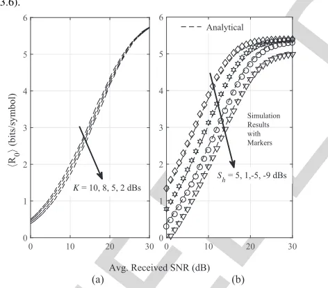
Fig. 7. Channel cutoff rate, R0of JFTS channel (with CSI) as a function of average received signal-to-noise ratio (a) with fixed Sh=1 dB,=0.4 and (b) with fixed K=5 dB,=0.9.

(refer to Fig. 7(a)) is much less compared to the decrease in 556

achievable cutoff rate due to the lowering of Sh-factor from

557

5 dB to −5 dB (refer to Fig. 7(b)). These results do not 558

agree with the observations made in [20], where bit error rate 559

performance of BPSK is found to degrade equally either due 560

to the decrease in the K -factor or the Sh-factor. The reason for

561

this can be attributed to the-value chosen for each plot. For 562

Fig. 7(a), a low of 0.4 is chosen. In this case, shadowing 563

severity is reduced by the fact that only one scattering cluster 564

dominates instead of two clusters. For Fig. 7(b) a high of 565

0.9 is chosen, where the magnitudes of the shadowing values 566

contributed by each scattering cluster are almost equal. 567

Fig. 8. Channel cutoff rate, R0of JFTS channel under different modulation techniques (a) with different constellation size M and (b) presence/absence of CSI with K=7 dB, Sh=6 dB and=0.7.

It is worth mentioning that the channel cutoff results 568 plotted in Fig. 7 are analytical results, as these results are 569 only estimates of the achievable throughput, neither exact 570 nor approximate bounds on the actual system performance. 571 However, we have plotted the achievable throughput over JFTS 572 channel with K = 5 dB, Sh = −9 dB, = 0.9 through 573 Monte-Carlo simulation for comparison. Plotting simulation 574 results for all values of K and Sh have been avoided due to 575

space constraint. 576

2) Performance of Modulation Techniques: Fig. 8 demon- 577 strates the cutoff rate for different modulation schemes in the 578 JFTS channel. The curves in Fig. 8(a) are used to compare 579 performances of M-QAM/PSK over JFTS faded / shadowed 580 communication links with K =7 dB, Sh=6 dB and=0.7. 581 The channel cutoff rate curves are generated using (17). The 582 unrestricted upper bound or the average achievable channel 583 capacity under this particular channel condition is also plotted 584 for reference. In this case, the unrestricted upper bound on 585 achievable channel capacity over a JFTS fading/shadowing 586 channel can be evaluated using CJFTS = EZ

Bτ log2(1+ 587

zγ ) [bits/symbol], where the expectation is taken over z, 588

[image:8.612.65.301.360.567.2]

IEEE Proof

of the presence of shadowing. Therefore, though there still

605

exists a group of waves arriving directly at the receiver over 606

the LOS path, they are obstructed due to the presence of 607

in-building structures like the thin set of dry-walls between 608

the transmitter and the receiver. 609

However, for the JFTS channel, QAM without CSI still 610

performs better than PSK, as is the case in the presence of 611

perfect CSI (refer to Fig. 8(b)). This contrasting behavior 612

between outdoor and indoor channels can be attributed to that 613

fact that in an indoor environment, shadowing varies quickly 614

enough to have an impact on the decision region boundaries 615

along with fading. In case of PSK receivers, the decision 616

boundaries are not independent of the shadowing depth and 617

therefore performs equally poorly as QAM receivers over a 618

JFTS faded/shadowed communication link. 619

VI. CONCLUSIONS

620

The primary contribution of this paper is to derive easy-to-621

evaluate closed-form analytical expressions for the ABER of a 622

wireless communication system using M-QAM and coherent 623

M-PSK modulation techniques over JFTS fading / shadowing

624

channels. In order to do so, closed-form expressions for the 625

PDF and the CDF of the received instantaneous composite 626

signal-to-noise ratio (SNR) are utilized. The derived analytical 627

expressions for ABER are numerically evaluated and plotted 628

as functions of the parameters of the communication channel 629

model and the modulation techniques. Performance degrades 630

as K and Shdecreases and enhances asdecreases. The

ana-631

lytical results are found to be in agreement with the simulation 632

results verifying the validity of the derived expressions. It can 633

also be concluded that for higher SNRs, performance over a 634

JFTS channel model is better than the NL channel model for 635

the same AF. 636

APPENDIXA 637

PROOF OFPROPOSITION1 638

The CDF of γ can be defined as 639

F_γ(γ )=

_γ

−∞ fγ(u)du=1−

_∞

γ fγ(u)du. (A.20) 640

Putting (5) back in (A.20), we can rewrite (A.20) mathemati-641

cally as 642

F_γ(γ ) =1−

4

i=1

m

h=1

∞

t=0 Ai_,h

γ (t!)2

C1iC

t

3i

γt +C2i

C_4it

γt 643 × _∞ γ u

t_e−Bh_γu_du

. (A.21) 644

Using the integral solution from [17, p. 340, eq. (3.351.2)], 645

we can express (A.20) as 646

F_γ(γ ) =1−

4

i=1

m

h=1

∞

t=0 Ai,h

γ (t!)2

C1iC

t

3i

γt +C2i

C_4it

γt 647 × _γ Bh t₊1

t+1,Bhγ

γ

648

=1−

4

i=1

m

h=1

∞

t=0

Ai,h(t+1,Bhγ /γ )

(t!)2_Bt+1

h

649

×

C1iC_3it +C2iCt_4i

. (A.22) 650

Following the same steps as above, we can arrive at the 651 approximate form of F_γ(γ )as 652

F_γ(γ )≈1−

4

i=1

m

h=1

tmax

t=0

Ai,h(t+1,Bhγ /γ )

(t!)2_Bt+1

h

653

×

D1tC1iC_3it +D2tC2iC_4it

. (A.23) 654

The results obtained in (A.22) and (A.23) are put back in (7) 655 to obtain the final expressions in Proposition 1. 656

APPENDIXB 657

PROOF OFPROPOSITION2 658 Starting from (8) and putting back the first line of (7) back 659 in (8), we can rewrite (8) as 660

P_bBinary(e)= α β

2(β)

_∞

0

γβ−1 e−αγ

1−

4

i=1

m

h=1

∞

t=0 Ai,h

(t!)2 661

×(t+1,Bhγ /γ )

B_ht+1

C1iC_3it +C2iC_4it

dγ. 662

(B.24) 663

Using the integral solution from[17, p. 340, eq. (3.351.3)], we 664 can express (B.24) as 665

P_bBinary(e)= 1

2 −

4

i=1

m

h=1

∞

t=0 Ai,h

(t!)2_Bt+1

h

C1iC_3it +C2iC_4it

666

× αβ

2(β)

_∞

0

γβ−1_e−αγ_(t+1,B

hγ /γ )dγ

. 667 (B.25) 668

Using the integral solution from [17, eq. 6.455.1, p. 657], we 669

can obtain 670

P_bBinary(e)= 1

2−

4

i=1

m

h=1

∞

t=0 Ai,h

(t!)2

C1iC_3it +C2iC_4it

671

× αβγβ

2β(β)

(β+t+1) (αγ +Bh)β+t+1

672

×2F1

1, β+t+1;β+1; αγ αγ +Bh

. 673

(B.26) 674

Following the same steps as above and putting the second line 675 of (7), we can arrive at the approximate form of P_bBinary(e)as 676

P_bBinary(e)≈ 1

2−

4

i=1

m

h=1

tmax

t=0 Ai_,h

(t!)2

D1tC1iC_3it +D2tC2iC_4it

677

× αβγβ

2β(β)

(β+t+1) (αγ +Bh)β+t+1

678

×2F1

1, β+t+1;β+1; αγ αγ +Bh

. 679

IEEE Proof

The results obtained in (B.26) and (B.27) are put back in (9)

681

to obtain the final expressions in Proposition 2. 682

APPENDIXC 683

PROOF OFPROPOSITION3 684

Starting from (10) and putting back the first line of (7) back 685

in (10), we can rewrite (10) as 686

P_bM−ary(e,g)= √1

2

_∞

0

e−v2/2

1−

4

i=1

m

h=1

∞

t=0 Ai,h

(t!)2

687

×(t+1,Bhv2/gγ ) B_ht+1

C1iC_3it +C2iC_4it

dγ. 688

(C.28) 689

Using the integral solution from [17, p.340, eq. (3.351)], we 690

can express (C.28) as 691

P_bM-ary(e,g)= 1

2 −

4

i=1

m

h=1

∞

t₌0 Ai,h

(t!)2_Bt+1

h

C1iC3it +C2i

692

×Ct_4i

1

√

2

_∞

0

e−v2/2(t+1,Bhv2/gγ )dγ

. 693

(C.29) 694

Puttingv2=r with change of variables and using the integral

695

solution from [17, p. 657, eq. (6.455.1)], we can obtain 696

P_bM-ary(e,g)

697

= 1

2−

4

i=1

m

h=1

∞

t=0 Ai_,h

(t!)2

C1iC_3it +C2iC_4it

698

×2t+1 √

gγ (t+3/2) (gγ+2Bh)t+3/2

2F1

1,t+3

2; 3 2;

gγ gγ+2Bh

. 699

(C.30) 700

Following the same steps as above and putting the second line 701

of (7), we can arrive at the approximate form of P_bM-ary(e,g)

702 as 703

P_bM-ary(e,g)

704

≈ 1

2 −

4

i=1

m

h=1

tmax

t=0

D1tC1iC_3it +D2tC2iC_4it

705

×Ai,h

(t!)2

2t+1√gγ (t+3/2) (gγ+2Bh)t+3/2

2F1

1,t+3

2; 3 2;

gγ gγ+2Bh

. 706

(C.31) 707

The results obtained in (C.30) and (C.31) are put back in (11) 708

to obtain the final expressions in Proposition 3. 709

REFERENCES

710

[1] H. Suzuki, “A statistical model for urban radio propogation,” IEEE

711

Trans. Commun., vol. COM-25, no. 7, pp. 673–680, Jul. 1977.

712

[2] T. T. Tjhung and C. C. Chai, “Fade statistics in Nakagami-lognormal

713

channels,” IEEE Trans. Commun., vol. 47, no. 12, pp. 1769–1772,

714

Dec. 1999.

715

[3] P. S. Bithas, N. C. Sagias, P. T. Mathiopoulos, G. K. Karagiannidis,

716

and A. A. Rontogiannis, “On the performance analysis of digital

717

communications over generalized-K fading channels,” IEEE Commun.

718

Lett., vol. 10, no. 5, pp. 353–355, May 2006.

719

[4] I. Dey, G. G. Messier, and S. Magierowski, “Joint fading and shadowing 720

model for large office indoor WLAN environments,” IEEE Trans. 721

Antennas Propag., vol. 62, no. 4, pp. 2209–2222, Apr. 2014. 722

[5] G. D. Durgin, T. S. Rappaport, and D. A. D. Wolf, “New analytical 723

models and probability density functions for fading in wireless com- 724

munications,” IEEE Trans. Commun., vol. 50, no. 6, pp. 1005–1015, 725

Jun. 2002. 726

[6] I. Dey, G. G. Messier, and S. Magierowski, “Fading statistics for the 727

joint fading and two path shadowing channel,” IEEE Wireless Commun. 728

Lett., vol. 3, no. 3, pp. 301–304, Jun. 2014. 729

[7] I. Dey, G. G. Messier, and S. Magierowski, “The cumulative distribution 730

function for the joint fading and two path shadowing channel: Expression 731

and application,” in Proc. IEEE VTC-Fall, Sep. 2014, pp. 1–5. 732

[8] I. Dey, G. G. Messier, and S. Magierowski, “On the capacity of joint 733

fading and two-path shadowing channels,” IEEE Trans. Veh. Technol., 734

vol. 65, no. 1, pp. 403–408, Jan. 2016. 735

[9] G. P. Efthymoglou, N. Y. Ermolova, and V. A. Aalo, “Channel 736

capacity and average error rates in generalised-K fading channels,” 737

IET Commun., vol. 4, no. 11, pp. 1364–1372, Jul. 2010. 738

[10] I. Dey, T. A. Tsiftsis, and C. Rowell, “Achievable channel cutoff rate 739

and bandwidth efficiency in indoor wireless environments,” IEEE Trans. 740

Veh. Technol., vol. 65, no. 12, pp. 10074–10079, Dec. 2016. 741

[11] W. T. Webb, L. Hanzo, and R. Steele, “Bandwidth efficient QAM 742

schemes for Rayleigh fading channels,” IEE Proc. I-Commun., Speech 743

Vis., vol. 138, no. 3, pp. 169–175, Jun. 1991. 744

[12] M. Abramowitz and I. A. Stegun, Handbook of Mathematical Functions: 745

With Formulas, Graphs, and Mathematical Tables, 9th ed. New York, 746

NY, USA: Dover, 1972. 747

[13] M. K. Simon and M.-S. Alouini, Digital Communication Over Fading 748

Channels, 2nd ed. Hoboken, NJ, USA: Wiley, 2005. 749

[14] Y. Zhao, P. Adve, and T. J. Lim, “Symbol error rate of selection amplify- 750

and-forward relay systems,” IEEE Commun. Lett., vol. 10, no. 11, 751

pp. 757–759, Nov. 2006. 752

[15] A. Abdi and M. Kaveh, “Comparison of DPSK and MSK bit error rates 753

for K and Rayleigh-lognormal fading distributions,” IEEE Commun. 754

Lett., vol. 4, no. 4, pp. 122–124, Apr. 2000. 755

[16] R. Steele and L. Hanzo, Mobile Radio Communications: Second and 756

Third-Generation Cellular and WATM Systems, 2nd ed. New York, NY, 757

USA: Wiley, 1999. 758

[17] I. S. Gradshteyn and I. M. Ryzhik, Table of Integrals, Series, and 759

Products, 7th ed. New York, NY, USA: Elsevier, 2007. 760

[18] C. Schlegel and D. J. Costello, Jr., “Bandwidth efficient coding for fading 761

channels: Code construction and performance analysis,” IEEE J. Sel. 762

Areas Commun., vol. 7, no. 9, pp. 1356–1368, Dec. 1989. 763

[19] D. Divsalar and M. Simon, “Trellis coded modulation for 764

4800–9600 bits/s transmission over a fading mobile satellite channel,” 765

IEEE J. Sel. Areas Commun., vol. SAC-5, no. 2, pp. 162–177, Feb. 1987. 766

[20] I. Dey, G. G. Messier, and S. Magierowski, “Performance analysis of 767

BPSK over joint fading and two-path shadowing channels,” in Proc. 768

IEEE VTC-Fall, Sep. 2014, pp. 1–5. 769

[21] W. T. Webb and R. Steele, “Variable rate QAM for mobile radio,” IEEE 770

Trans. Commun., vol. COM-43, no. 7, pp. 2223–2230, Jul. 1995. 771

Indrakshi Dey received the B.Tech. degree (Hons.) 772

in electronics and communication engineering from 773

the West Bengal University of Technology, Kolkata, 774

India, in 2005, the M.Sc. degree in wireless com- 775

munications from the University of Southampton, 776

Southampton, U.K., in 2010, and the Ph.D. degree 777

in electrical engineering from the University of 778

Calgary, Calgary, Canada, in 2015. From 2015 to 779

2016, she was a Post-Doctoral Research Fellow with 780

the Ultra-Maritime Digital Communication Center, 781

Dalhousie University, Halifax, Canada. She was a 782

Research Fellow with the Department of Electronics and Telecommunications, 783

Norwegian University of Science and Technology, Trondheim, Norway, from 784

2016 to 2017. Her current research interests include channel modeling, 785

channel estimation and prediction, adaptive modulation, and dirty tape coding 786

for different wireless propagation environments, and wireless sensor networks. 787

In 2016, she received the prestigious research fellowship from the European 788

IEEE Proof

Geoffrey G. Messier received the B.S. degree

790

(Hons.) in electrical engineering and the B.S. degree

791

(Hons.) in computer science from the University of

792

Saskatchewan, Canada, in 1996, the M.Sc. degree

793

in electrical engineering from the University of

794

Calgary, Canada in 1998, and the Ph.D. degree in

795

electrical and computer engineering from the

Uni-796

versity of Alberta, Canada, in 2004. From 1998 to

797

2004, he was with the Nortel Networks CDMA Base

798

Station Hardware Systems Design Group, Calgary,

799

Canada. At Nortel Networks, he was responsible for

800

radio channel propagation measurements and simulating the physical layer

801

performance of high speed CDMA and multiple antenna wireless systems.

802

He is currently an Associate Professor with the Department of Electrical and

803

Computer Engineering, University of Calgary. His research interests include

804

data networks, physical layer communications, and communications channel

805

propagation measurements.

806

Sebastian Magierowski received the Ph.D. degree 807

in electrical engineering from the University of 808

Toronto in 2004. From 2004 to 2012, he served as an 809

Assistant/Associate Professor with the Department 810

of Electrical and Computer Engineering, University 811

of Calgary, after which, he joined the Faculty of the 812

Department of Electrical Engineering and Computer 813

Science with the Lassonde School of Engineer- 814

ing, York University, Toronto, Canada, where he 815

is currently an Associate Professor. As part of his 816

industrial experience (Nortel Networks, PMC-Sierra, 817

and Protolinx Corporation), he has involved in CMOS device modeling, 818

high-speed mixed-signal IC design, and data networks. His research interests 819

include analog/digital CMOS circuit design, communication systems, and 820