Analysis of Composite Runge Kutta Methods and New One-Step Technique for Stiff Delay Differential Equations

Analysis of Composite Runge Kutta Methods and

New One-Step Technique for Stiff Delay Differential

Equations

1

J. Vinci Shaalini, 2*A. Emimal Kanaga Pushpam

Abstract- This paper presents fourth order Composite Runge

Kutta (RK) methods based on Arithmetic Mean (AM), Harmonic Mean (HaM), Centroidal Mean (CeM), Contraharmonic Mean (CoM) and a new one-step technique which uses non-linear polynomial interpolating function to solve the stiff Delay differential equations (DDEs). The stability polynomials of these methods are derived. The Local Grid Search Algorithm is used to determine the stability regions. The efficiency of these methods is compared through three numerical examples of stiff Delay Differential Equations (DDEs).

Index Terms- Stiff Delay Differential Equations, Means, New

One-Step technique, Lagrange Interpolation, Stability polynomial and region.

I. INTRODUCTION

Delay differential equations have been rapidly developing in chemical kinetics[1], population dynamics [2], management systems [3] and in several areas of science and engineering. Recently there has been a growing interest in the numerical solutions of DDEs. Ismail and Read Ali [4] obtained the numerical solution of DDEs by RK method by using Hermite interpolation. Fatemeh [5] and Rostann [6] et al proposed homotopy perturbation and adomian decomposition methods. Radzi [7] et al investigated the two and three point one-step block method for solving DDEs. Toheeb et al. [8] found the exact solution by using the combination of Laplace and the variational iteration method. Ismail and Suleiman [9] studied the p-stability and q-stability of singly diagonally implicit Runge-Kutta method for DDEs.

Many researchers have tried to extend and modify the RK methods according to their needs. This is because of the nature of flexibility, efficiency and accuracy. In this way, RK methods based on variety of means have been developed by Murugesan et al. [10, 11] in ordinary differential equations (ODEs). Dingwen and Tingting [12] developed the fourth order singly diagonally implicit Runge-Kutta method for solving one-dimensional Burger’s equations.

Manuscript received July 18, 2018; revised February 28, 2019.

1_{J. Vinci Shaalini is with the Mathematics Department, Bishop Heber}

College, Tiruchirappalli 620017, Tamilnadu, India. e-mail: [email protected].

2*_{A. Emimal Kanaga Pushpam is with the Mathematics Department, Bishop}

Heber College, Tiruchirappalli 620017, Tamilnadu, India. e-mail: [email protected].

Several one-step techniques using variety of interpolating polynomials and functions have been developed to solve ODEs. In 1976, Fatunla [13] gave a new algorithm which consists of the interpolating function of two complex parameters for solving ordinary differential equations. Kama and Ibijola [14] have developed the new one-step polynomial and exponential interpolating function technique for solving initial value problems in ordinary differential equations. In 2017, Abolarin et al. [15] derived the fourth stage inverse polynomial scheme to initial value problems. Fadugba and Falodun [16] have developed the new one-step power series polynomial scheme for initial value problems in ODEs. In 2000, Asgari found the numerical solution for solving a system of fractional integro-differential equations [17].

Most of the models in differential equations are ‘stiff’ in nature. For solving stiff equations, the step size is taken to be extremely small. Also, many problems may be stiff in some intervals and non-stiff in others. Several numerical methods have been used for solving stiff DDEs. In 1980, Roth [18] investigated the difference method for stiff delay differential equations. Bocharov [19] gave the numerical solution by LMMs of stiff delay differential systems modelling immune response. El-Safty [20] and Zhu [21] have found the Chebyschev method and parallel two-step ROW methods for stiff delay differential equations.

The purpose of this study is to present Composite RK methods based on different means such as AM, CeM, HaM, CoM and a new one-step technique which uses non-linear polynomial interpolating function while solving DDEs. Lagrange interpolation is used to approximate the delay argument. The stability polynomials are derived for these numerical methods. Their corresponding stability regions are also plotted.

II. FOURTH ORDER COMPOSITE RK METHODS FOR ODES

Consider the first order equation of the form

𝑦′_{= 𝑓(𝑥, 𝑦) with 𝑦(𝑥} 0) = 𝑦0

The classical fourth order RK method is given by

𝑦𝑛+1 = 𝑦𝑛+ ℎ

6[𝑘1+ 2𝑘2+ 2𝑘3+ 𝑘4] (1)

which involve 𝑘𝑖, 1 ≤ 𝑖 ≤ 4, given by

IAENG International Journal of Applied Mathematics, 49:3, IJAM_49_3_14

𝑘𝑖= 𝑓(𝑡𝑛+ 𝑐𝑖ℎ, 𝑦𝑛+ ℎ ∑𝑖𝑗=1𝑎𝑖𝑗𝑘𝑗) where 𝑐𝑖= ∑𝑖𝑗=1𝑎𝑖𝑗

The formula (1) can be rewritten as

𝑦𝑛+1= 𝑦𝑛+ ℎ

3∑ [

𝑘_𝑖+𝑘_𝑖+1

2 ] = 𝑦𝑛+ ℎ

3[∑ (AM)

3

𝑖=1 ]

3

𝑖=1 (2)

The above formula (2) can be called as the fourth order RKAM formula. The values of AM can be replaced by variety of means such as HaM, CeM and CoM which are given in Table I. The formulae for HaM, CeM and CoM in terms of AM and GM and also the corresponding values of and in all these cases can be referred in Murugesan et al [11].

III. FOURTH ORDER COMPOSITE RK METHODS FOR DDES

In this section, the fourth order RK formulae have been extended to solve DDEs with constant delays. Consider the first order DDEs with constant delay



,

𝑦′_{(𝑡) = 𝑓 (𝑡, 𝑦(𝑡), 𝑦 (𝑡 − 𝜏(𝑡, 𝑦(𝑡)))) , 𝑡 > 𝑡} 0

𝑦(𝑡) = Φ(𝑡), 𝑡 ≤ 𝑡0

where Φ(𝑡) is the initial function. The fourth order RK method using variety of means can be written as

𝑦𝑛+1= 𝑦𝑛+ ℎ

3[∑ 𝑀𝑒𝑎𝑛𝑠 3

𝑖=1 ]

which involve 𝑘𝑖, 1 ≤ 𝑖 ≤ 4, given by

𝑘𝑖= 𝑓 (𝑡𝑛+ 𝑐𝑖ℎ, 𝑦𝑛+ ℎ ∑𝑖𝑗=1𝑎𝑖𝑗𝑘𝑗, 𝑦(𝑡𝑛+ 𝑐𝑖ℎ − 𝜏))

where 𝑐𝑖= ∑𝑖𝑗=1𝑎𝑖𝑗

Here Means include AM, HaM, CeM and CoM. The fourth order RK formulae based on various means for solving DDEs are same as given in Table I. These RK formulae can also be extended to solve DDEs with multiple delays. In this paper, Lagrange interpolation is used to approximate the delay argument.

IV. ANALYSIS OF COMPOSITE RK METHODS

A. ORDER OF CONVERGENCE OF COMPOSITE RK METHODS

The interpolation order and hence the number of support points have to be adapted to the order of the method. For any given RK method, its adaptation to DDEs by means of interpolation procedure has an order of convergence equal to min{p, q}where p denotes the order of consistency of the RK method and q is the number of support points of the interpolation procedure [22]. Here we use four support points of Lagrange interpolation so that the order of convergence of RK method is four for DDEs also.

B. STABILITY ANALYSIS OF COMPOSITE RK METHODS

The stability of numerical methods to DDEs depends on the test equation and the delay term involved. Here we consider a commonly used linear test equation with a constant delay 𝜏 = 1 where N is a positive integer,

𝑦′_{(𝑡) = 𝜆𝑦(𝑡) + 𝜇𝑦(𝑡 − 𝜏), 𝑡 ≥ 0}

𝑦(𝑡) = Φ(𝑡), 𝑡 ∈ [−𝜏, 0] (3)

where 𝜆, 𝜇 ∈ 𝐶, 𝜏 > 0, and Φ _{is continuous.}

Assume that the numerical solution has been calculated up to

point

t

n with uniform step size h, satisfying 𝜏 = 𝑁ℎ, where N

is a positive integer. Lagrange interpolation is used to approximate the delay term using previously calculated value of y, giving

𝑦(𝑡𝑛+ 𝑐𝑖ℎ − 𝑁ℎ) = 𝑦(𝑡𝑛−𝑁+ 𝑐𝑖ℎ)

= ∑ 𝐿𝑙(𝑐𝑖)𝑦𝑛−𝑁+𝑙 𝑠1

𝑙=−𝑟1 (4)

with 𝐿𝑙(𝑐𝑖) = ∏ 𝑐_𝑙−𝑗𝑖−𝑗1

1, 𝑗1≠ 𝑙 𝑎𝑛𝑑 𝑟1, 𝑠1 > 0

𝑠1

𝑗1=−𝑟1

and 𝑦𝑛−𝑁+𝑙 is calculated value of 𝑦(𝑡𝑛−𝑁+𝑙). When RK method

is applied to DDE (3) with delay 𝜏 = 1, the following equations are obtained.

𝑘𝑖= 𝑓(𝑡𝑛+ 𝑐𝑖ℎ, 𝑦𝑛+ ℎ ∑ 𝑎𝑖𝑗𝑘𝑖, ∑𝑠𝑙=−𝑟1 1𝐿𝑙(𝑐𝑖)𝑦𝑛−𝑁+𝑙 𝑞

=1 ) (5)

𝑦𝑛+1= 𝑦𝑛+ ℎ ∑ 𝑎𝑖𝑗𝑘𝑖 𝑞 𝑖=1

Define

u





1,...,1



T,





T (1) (2) (q)

,

,...,

k

k

k



k

,





T

1, ,...,2 q and

b b b



b L (c)_l 



L_l(c ),...,₁ L_l(c ) ._q



T

For 𝑛 ≥ 𝑁, considering f as in (3), (5) can be written as

𝐤 = 𝜆(𝑦𝑛𝐮 + ℎ𝐴𝑘) + 𝜇(∑ 𝐋𝐥(𝐜)𝑦𝑛−𝑁+𝑙) (6)

𝑦𝑛+1 = 𝑦𝑛+ ℎ𝐛𝐓𝐤 (7)

From equation (6),

𝐤 = 𝜆𝑦𝑛𝐮[𝐼 − 𝜆ℎ𝐴]−1+ 𝜇[𝐼 − 𝜆ℎ𝐴]−1∑ 𝐋𝐥(𝐜)𝑦𝑛−𝑁+𝑙

ℎ𝐤 = 𝛼𝑦_𝑛𝐮𝜂 + 𝛽𝜂∑𝐋𝐥(𝐜)𝑦𝑛−𝑁+𝑙 (8)

where 𝛼 = 𝜆ℎ, 𝛽 = 𝜇ℎ, 𝜂 = [𝐼 − 𝜆ℎ𝐴]−1 _{and I is the identity} matrix.

Substituting (8) in (7),

𝑦𝑛+1 = 𝑦𝑛+ 𝛼𝐛𝐓𝜂𝑦𝑛𝐮 + 𝛽𝐛𝐓𝜂 ∑𝐋𝐥(𝐜)𝑦𝑛−𝑁+𝑙 (9)

Taking 𝐘𝐧 = (𝑦𝑛, ℎ𝐤)𝑇 (8) and (9) can be written as the

recurrence,

n N l 



n+1 n

Y

XY + ZY

where

IAENG International Journal of Applied Mathematics, 49:3, IJAM_49_3_14

T T

1 0,..., 0 0

0 0 . . and . . . . 0 0                                               





l l

b u b L (c)

X Z

u L (c)

By putting n  N l 0, the stability polynomial will be in the standard form. The recurrence is stable if the zeros



_i of the stability polynomial





1

1

1 1

, ,

det

s

n n l

l l r

S

  





I



X





Z























and

satisfies the root condition



_i



1.

To obtain the stability region of the method, we used four points interpolation to evaluate

y t



_n



c h

_i



1



. Then the stability polynomial for the method is,

𝑆(𝛼, 𝛽: 𝜁) = 𝜁𝑛+1_{−(1 + 𝛼𝐛}𝑇_{𝜂𝐮)𝜁}𝑛_{− 𝛽𝐛}𝑇_𝜂(𝐿

−1(𝑐) +

𝐿0(𝑐)𝜁 + 𝐿1(𝑐)𝜁2+ 𝐿2(𝑐)𝜁3)

To determine the stability polynomials for the RK method

based on variety of means, we need the dense output

b

 



where





(0, 1].

From the order conditions for 4-stage fourth order method, we obtained the fourth order interpolant as given in Table II. Generally, the stability polynomial for RK methods based on variety of means can be written as,

𝑆(𝛼, 𝛽: 𝜁) = 𝜁𝑛+1_{−(1 + 𝛼𝐛}𝑇_{(𝜃)𝜂𝐮)𝜁}𝑛

−𝛽𝐛𝑇_{(𝜃)𝜂(𝐿}

−1(𝑐) + 𝐿0(𝑐)𝜁 + 𝐿1(𝑐)𝜁2+ 𝐿2(𝑐)𝜁3)

and they have been listed as follows.

For RKAM:

𝑆(𝛼, 𝛽: 𝜁) = 𝜁n+1_{− 𝜁}𝑛_{(1 + 𝛼 +}𝛼2

2 +

𝛼3

6 +

𝛼4 24) −

𝜁3₍−1

24𝛽 −

1

48𝛼𝛽 −

1 192𝛼

2_{𝛽) − 𝜁}2₍13 24𝛽 +

3

16𝛼𝛽 +

3 64𝛼

2_{𝛽) −}

𝜁 (13

24𝛽 + 17

48𝛼𝛽 +

25 192𝛼

2_{𝛽 +} 1 24𝛼

3_{𝛽) − (}−1

24𝛽 −

1

48𝛼𝛽 −

1 192𝛼

2_𝛽)

For RKHaM:

𝑆(𝛼, 𝛽: 𝜁) = 𝜁n+1_{− 𝜁}𝑛_{(1 + 𝛼 +}𝛼2

2 +

𝛼3

6 +

𝛼4 24) −

𝜁3₍−19

432𝛽 −

1

48𝛼𝛽 −

1 192𝛼

2_{𝛽) − 𝜁}2₍235

432𝛽 +

3

16𝛼𝛽 +

3 64𝛼

2_{𝛽) − 𝜁 (}235

432𝛽 +

17

48𝛼𝛽 +

25 192𝛼

2_{𝛽 +} 1 24𝛼

3_{𝛽) − (}−19

432𝛽 −

1

48𝛼𝛽 −

1 192𝛼

2_𝛽)

For RKCeM:

𝑆(𝛼, 𝛽: 𝜁) = 𝜁n+1_{− 𝜁}𝑛_{(1 + 𝛼 +}𝛼2

2 +

𝛼3

6 +

𝛼4 24)

−𝜁3₍−49 1168𝛽 −

1

48𝛼𝛽 −

1 192𝛼

2_{𝛽) − 𝜁}2₍633 1168𝛽 +

3

16𝛼𝛽 +

3 64𝛼

2_{𝛽) − 𝜁 (}633 1168𝛽 +

17

48𝛼𝛽 +

25 192𝛼

2_{𝛽 +} 1 24𝛼

3_{𝛽) − (}−49 1168𝛽 − 1

48𝛼𝛽 −

1 192𝛼

2_𝛽)

For RKCoM:

𝑆(𝛼, 𝛽: 𝜁) = 𝜁n+1_{− 𝜁}𝑛_{(1 + 𝛼 +}𝛼2

2 +

𝛼3

6 +

𝛼4 24)

−𝜁3₍−19

432𝛽 −

1

48𝛼𝛽 −

1 192𝛼

2_{𝛽) − 𝜁}2₍235

432𝛽 +

3

16𝛼𝛽 +

3 64𝛼

2_{𝛽) − 𝜁 (}235

432𝛽 +

17

48𝛼𝛽 +

25 192𝛼

2_{𝛽 +} 1 24𝛼

3_{𝛽) − (}−19

432𝛽 −

1

48𝛼𝛽 −

1 192𝛼

2_𝛽)

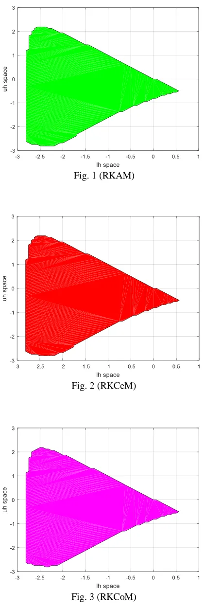
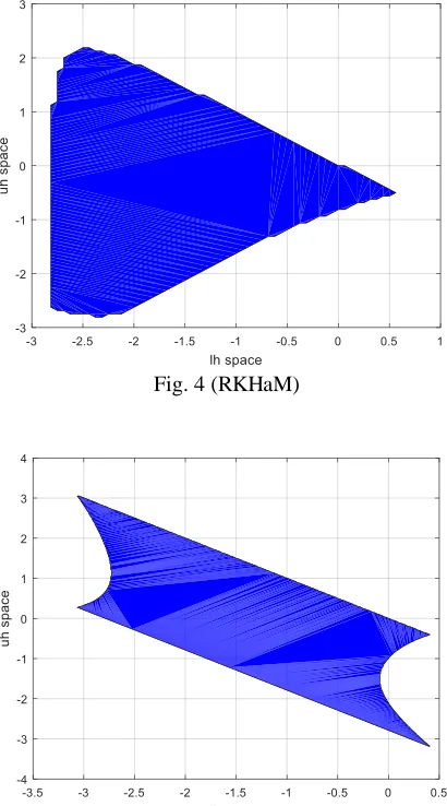
Their corresponding stability regions are given in Fig. 1-4.

V. A NEW ONE-STEP TECHNIQUE FOR SOLVING DDEs

Let us assume that the analytical solution 𝑦(𝑡) to the initial value problem (1) can be locally represented in the interval [𝑡𝑛, 𝑡𝑛+1], 𝑛 ≥ 0 by the non-linear polynomial interpolating

function

𝐹(𝑡) = 𝑎1𝑒2𝑡+ 𝑎2𝑡4+ 𝑎3𝑡3+ 𝑎4 𝑡2+ 𝑎5 𝑡 + 𝑎6 (10)

where 𝑎1, 𝑎2 𝑎3, 𝑎4, 𝑎5 and 𝑎6 are undetermined coefficients.

We shall assume 𝑦𝑛 is a numerical approximation to the

analytical solution 𝑦(𝑡) and using mesh points as follows:

𝑡𝑛= 𝑎 + 𝑛ℎ, 𝑛 = 0,1,2, … (11)

Taking the following constraints on the interpolating function (3) in order to get the undetermined coefficients.

Firstly, the interpolating function must coincide with the analytical solution at

𝑡 = 𝑡𝑛 and 𝑡 = 𝑡𝑛+1.

Hence we required that

𝐹(𝑡𝑛) = 𝑎1𝑒2𝑡𝑛+ 𝑎2𝑡𝑛4+ 𝑎3𝑡𝑛3+ +𝑎4𝑡𝑛2+ 𝑎5𝑡𝑛+ 𝑎6

(12) and

𝐹(𝑡𝑛+1) = 𝑎1𝑒2𝑡𝑛+1+ 𝑎2𝑡𝑛+14+ 𝑎3𝑡𝑛+13+ 𝑎4𝑡𝑛+12

+𝑎5𝑡𝑛+1+ 𝑎6 (13)

Secondly, the derivatives of the interpolating function are required to coincide with the differential equation as its first, second, and third derivatives with respect to t at 𝑡 = 𝑡𝑛. We

denote the ith _{total derivatives of 𝑓(𝑡, 𝑦(𝑡), 𝑦(𝑡 − 𝜏(𝑡, 𝑦(𝑡))))}

with respect to t with 𝑓(𝑖) _{such that}

𝐹1_(𝑡 𝑛) = 𝑓𝑛

(1)

(14)

IAENG International Journal of Applied Mathematics, 49:3, IJAM_49_3_14

𝐹2_(𝑡 𝑛) = 𝑓𝑛

(2)

(15)

𝐹3_(𝑡 𝑛) = 𝑓𝑛

(3)

(16)

𝐹4_(𝑡 𝑛) = 𝑓𝑛

(4)

(17)

𝐹5_(𝑡 𝑛) = 𝑓𝑛

(5)

(18)

𝑓𝑛 (1)

= 2𝑎1𝑒2𝑡𝑛+ 4𝑎2𝑡𝑛3+ 3𝑎3𝑡𝑛2+ 2𝑎4𝑡𝑛+ 𝑎5 (19)

𝑓_𝑛(2)= 4𝑎1𝑒2𝑡𝑛+ 12𝑎2𝑡𝑛2+ 6𝑎3𝑡𝑛+ 2𝑎4 (20)

𝑓_𝑛(3)= 8𝑎1𝑒2𝑡𝑛+ 24𝑎2𝑡𝑛+ 6𝑎3 (21)

𝑓_𝑛(4)= 16𝑎1𝑒2𝑡𝑛+ 24𝑎2 (22)

𝑓_𝑛(5)= 32𝑎1𝑒2𝑡𝑛 (23)

solving for 𝑎1from eqn. (23), we have

𝑎1= 𝑓_𝑛(5)

32𝑒2𝑡𝑛 (24)

Substituting (24) in (22), we have

𝑎2= 1 24[𝑓𝑛

(4)

−𝑓𝑛(5)

2 ] (25)

Substituting (24) and (25) into (21), we have

𝑎3= 1 6[(𝑓𝑛

(3)

−𝑓𝑛 (5)

4 ) − (𝑓𝑛 (4)

−𝑓𝑛 (5)

2 ) 𝑡𝑛] (26)

Substituting (24), (25) and (26) into (20), we have

𝑎4= 1 2[

(𝑓_𝑛(2)−𝑓𝑛(5) 8 ) − (𝑓𝑛

(3)

−𝑓𝑛(5) 4 ) 𝑡𝑛

− (𝑓𝑛(5)

4 −

𝑓_𝑛(4) 2 ) 𝑡𝑛

2

] (27)

Substituting (24), (25), (26) and (27) into (19), we have

𝑎5= [

(𝑓_𝑛(1)−𝑓𝑛(5) 16) − (𝑓𝑛

(2)₋𝑓_𝑛(5) 8 ) 𝑡𝑛

− (𝑓𝑛(5)

8 −

𝑓_𝑛(3) 2 ) 𝑡𝑛

2_{− (}𝑓𝑛(4)

6 −

𝑓_𝑛(5) 12) 𝑡𝑛

3

] (28)

Since 𝐹(𝑡𝑛+1) = 𝑦(𝑡𝑛+1) and 𝐹(𝑡𝑛) = 𝑦(𝑡𝑛) implies that

𝑦(𝑡𝑛+1) = 𝑦𝑛+1 and 𝑦(𝑡𝑛) = 𝑦𝑛

𝐹(𝑡𝑛+1) − 𝐹(𝑡𝑛) = 𝑦𝑛+1− 𝑦𝑛 (29)

Then we shall have

𝑦𝑛+1− 𝑦𝑛= 𝑎1𝑒2𝑡𝑛+1+ 𝑎2𝑡𝑛+14+ 𝑎3𝑡𝑛+13+ 𝑎4𝑡𝑛+12

+𝑎5𝑡𝑛+1+ 𝑎6− (𝑎1𝑒2𝑡𝑛+ 𝑎2𝑡𝑛4+ 𝑎3𝑡𝑛3

+𝑎4𝑡𝑛2+ 𝑎5𝑡𝑛+ 𝑎6)

= 𝑎1(𝑒2𝑡𝑛+1− 𝑒2𝑡𝑛) + 𝑎2(𝑡𝑛+14− 𝑡𝑛4)

+𝑎3(𝑡𝑛+13− 𝑡𝑛3) + 𝑎4(𝑡𝑛+12− 𝑡𝑛2)

+𝑎5(𝑡𝑛+1− 𝑡𝑛) (30)

Setting a = 0 in (11), we get 𝑡𝑛= 𝑛ℎ and 𝑡𝑛+1= (𝑛 + 1)ℎ

(31) Then,

𝑦𝑛+1= 𝑦𝑛+ 𝑎1(𝑒2𝑡𝑛+1− 𝑒2𝑡𝑛)

+𝑎2ℎ4(1 + 4𝑛 + 6𝑛2+ 4𝑛3)

+𝑎3ℎ3(1 + 3𝑛 + 3𝑛2) + 𝑎4ℎ2(1 + 2𝑛) + 𝑎5ℎ

(32) Eqn. (32) is the new one-step numerical technique.

This one-step technique can also be extended to solve DDEs with multiple delays. In this paper, Lagrange interpolation is used to approximate the delay argument.

VI. ANALYSIS OF NEW ONE-STEP TECHNIQUE

A. ORDER OF CONVERGENCE OF NEW ONE-STEP TECHNIQUE

A slight rearrangement of (32) and comparing with Taylor’s series,

𝑦𝑛+1= 𝑦𝑛+ ℎ𝑦𝑛′+

ℎ2

2 𝑦𝑛

′′₊ℎ 3

6 𝑦𝑛

′′′₊ℎ 4

24𝑦𝑛 (𝑖𝑣)

We found that the new one-step technique is of order four.

B. STABILITY ANALYSIS OF NEW ONE-STEP TECHNIQUE

A slight arrangement of (32), we obtain that

𝑦𝑛+1 = 𝑦𝑛+ ℎ𝑦𝑛′+ ℎ2

2 𝑦𝑛 ′′₊ℎ3

6 𝑦𝑛 ′′′₊ℎ4

24𝑦𝑛 (𝑖𝑣)

(33)

This implies,

𝑦𝑛+1 = 𝑦𝑛+ ℎ(𝜆𝑦𝑛+ 𝜇𝑦(𝑡𝑛− 𝜏))

+ ℎ 2

2 (𝜆𝑦

′

𝑛+ 𝜇𝑦

′_(𝑡 𝑛− 𝜏))

+ℎ3

6 (𝜆𝑦

′′

𝑛+ 𝜇𝑦

′′_(𝑡 𝑛− 𝜏))

+ℎ4

24(𝜆𝑦′′′𝑛+ 𝜇𝑦′′′(𝑡𝑛− 𝜏)) (34)

Here Lagrange interpolation is used to approximate the delay term.

𝑦(𝑡𝑛− 𝑚ℎ) = 𝑦(𝑡𝑛−𝑚) = ∑ 𝐿𝑙(𝑐𝑖)𝑦𝑛−𝑚+𝑙 𝑠1

𝑙=−𝑟1 with

𝐿𝑙(𝑐𝑖) = ∏

𝑐_𝑖−𝑗1

𝑙−𝑗1, 𝑗1≠ 𝑙 𝑎𝑛𝑑 𝑟1, 𝑠1 > 0 𝑠1

𝑗1=−𝑟1

Now 𝑦(𝑡𝑛− 𝜏) = ∑ 𝐿𝑙(𝑐)𝑦𝑛−𝑚+𝑙 𝑠1

𝑙=−𝑟₁ ,

𝑦′_(𝑡

𝑛− 𝜏) = 𝜆 ∑ 𝐿𝑙(𝑐)𝑦𝑛−𝑚+𝑙 𝑠₁

𝑙=−𝑟1

+𝜇 ∑ 𝐿𝑙(𝑐)𝑦𝑛−2𝑚+𝑙 𝑠1

𝑙=−𝑟1

𝑦′′_(𝑡

𝑛− 𝜏) = 𝜆 (

𝜆 ∑ 𝐿𝑙(𝑐)𝑦𝑛−𝑚+𝑙

𝑠1 𝑙=−𝑟₁

+𝜇 ∑ 𝐿𝑙(𝑐)𝑦𝑛−2𝑚+𝑙

𝑠₁ 𝑙=−𝑟1

)

+𝜇 ( 𝜆 ∑ 𝐿𝑙(𝑐)𝑦𝑛−2𝑚+𝑙

𝑠1 𝑙=−𝑟1

+𝜇 ∑ 𝐿𝑙(𝑐)𝑦𝑛−3𝑚+𝑙

𝑠1 𝑙=−𝑟1

)

IAENG International Journal of Applied Mathematics, 49:3, IJAM_49_3_14

and

𝑦′′′_(𝑡

𝑛− 𝜏) = 𝜆 (𝜆 (

𝜆 ∑ 𝐿𝑙(𝑐)𝑦𝑛−𝑚+𝑙

𝑠₁ 𝑙=−𝑟1

+𝜇 ∑ 𝐿𝑙(𝑐)𝑦𝑛−2𝑚+𝑙

𝑠1 𝑙=−𝑟1

) +

𝜇 ( 𝜆 ∑ 𝐿𝑙(𝑐)𝑦𝑛−2𝑚+𝑙

𝑠₁ 𝑙=−𝑟1

+𝜇 ∑ 𝐿𝑙(𝑐)𝑦𝑛−3𝑚+𝑙

𝑠1 𝑙=−𝑟1

)) +

𝜇 (𝜆 ( 𝜆 ∑ 𝐿𝑙(𝑐)𝑦𝑛−2𝑚+𝑙

𝑠₁ 𝑙=−𝑟1

+𝜇 ∑ 𝐿𝑙(𝑐)𝑦𝑛−3𝑚+𝑙

𝑠1 𝑙=−𝑟₁

) +

𝜇 ( 𝜆 ∑ 𝐿𝑙(𝑐)𝑦𝑛−3𝑚+𝑙

𝑠₁ 𝑙=−𝑟1

+𝜇 ∑ 𝐿𝑙(𝑐)𝑦𝑛−4𝑚+𝑙

𝑠1 𝑙=−𝑟₁

)) (35)

Substituting (35) in (34), we get

𝑦𝑛+1= 𝑦𝑛+ ℎ(𝜆𝑦𝑛+ 𝜇 ∑ 𝐿𝑙(𝑐)𝑦𝑛−𝑚+𝑙 𝑠1

𝑙=−𝑟1 )

+ℎ2

2 (

𝜆2_𝑦

𝑛+ 2𝜆𝜇 ∑ 𝐿𝑙(𝑐)𝑦𝑛−𝑚+𝑙 𝑠1

𝑙=−𝑟1

+𝜇2_{∑ 𝐿}

𝑙(𝑐)𝑦𝑛−2𝑚+𝑙 𝑠1

𝑙=−𝑟1

)

+ℎ3

6 (

𝜆3_𝑦

𝑛+ 3𝜆2𝜇 ∑ 𝐿𝑙(𝑐)𝑦𝑛−𝑚+𝑙

𝑠₁ 𝑙=−𝑟1

+3𝜆𝜇2_{∑ 𝐿}

𝑙(𝑐)𝑦𝑛−2𝑚+𝑙 𝑠1

𝑙=−𝑟1

+𝜇3_{∑ 𝐿}

𝑙(𝑐)𝑦𝑛−3𝑚+𝑙 𝑠₁

𝑙=−𝑟1

)

+ℎ4

24

( 𝜆4_𝑦

𝑛+ 4𝜆3𝜇 ∑ 𝐿𝑙(𝑐)𝑦𝑛−𝑚+𝑙

𝑠1 𝑙=−𝑟1 +6𝜆2_𝜇2_{∑ 𝐿}

𝑙(𝑐)𝑦𝑛−2𝑚+𝑙 𝑠1

𝑙=−𝑟1

+4𝜆𝜇3_{∑ 𝐿}

𝑙(𝑐)𝑦𝑛−3𝑚+𝑙 𝑠1

𝑙=−𝑟1

+𝜇4_{∑ 𝐿}

𝑙(𝑐)𝑦𝑛−4𝑚+𝑙 𝑠1

𝑙=−𝑟1 )

𝑦𝑛+1= 𝑦𝑛+ 𝜆ℎ𝑦𝑛+

𝜆2_ℎ2

2 𝑦𝑛+ 𝜆3_ℎ3

6 𝑦𝑛+ 𝜆4_ℎ4

24 𝑦𝑛 + ∑ 𝐿𝑙(𝑐)𝑦𝑛−𝑚+𝑙

𝑠1

𝑙=−𝑟₁ (𝜇ℎ + 𝜇𝜆ℎ2+

𝜆2𝜇ℎ3

2 +

𝜆3𝜇ℎ4

6 )

+ ∑ 𝐿𝑙(𝑐)𝑦𝑛−2𝑚+𝑙 𝑠1

𝑙=−𝑟₁ (

𝜇2ℎ2

2 +

𝜆𝜇2ℎ3

2 +

𝜆2𝜇2ℎ4

4 )

+ ∑ 𝐿𝑙(𝑐)𝑦𝑛−3𝑚+𝑙 𝑠₁

𝑙=−𝑟1 (

𝜇3ℎ3

6 +

𝜆𝜇3ℎ4

6 )

+ ∑ 𝐿𝑙(𝑐)𝑦𝑛−4𝑚+𝑙 𝑠1

𝑙=−𝑟1 (

𝜇4_ℎ4 24 )

Let 𝛼 = 𝜆ℎ and 𝛽 = 𝜇ℎ. Then the above equation becomes,

𝑦𝑛+1= 𝑦𝑛(1 + 𝛼 +

𝛼2 2!+ 𝛼3 3!+ 𝛼4 4!)

+ (𝛽 (1 + 𝛼 +𝛼2

2 +

𝛼3

6)) ∑ 𝐿𝑙(𝑐)𝑦𝑛−𝑚+𝑙

𝑠₁ 𝑙=−𝑟1

+ (𝛽2₍1

2+

𝛼

2+

𝛼2

4)) ∑ 𝐿𝑙(𝑐)𝑦𝑛−2𝑚+𝑙

𝑠1 𝑙=−𝑟₁

+ (𝛽3₍1

6+

𝛼

6)) ∑ 𝐿𝑙(𝑐)𝑦𝑛−3𝑚+𝑙

𝑠₁ 𝑙=−𝑟1

+ (𝛽4

24) ∑ 𝐿𝑙(𝑐)𝑦𝑛−4𝑚+𝑙

𝑠1 𝑙=−𝑟1

To obtain the stability region of the method, the delay term is approximated using four points Lagrange interpolation. By

putting 𝑛 − 𝑚 + 𝑙 = 0, 𝑛 − 2𝑚 + 𝑙 = 0, 𝑛 − 3𝑚 + 𝑙 = 0, 𝑛 − 4𝑚 + 𝑙 = 0 and by taking 𝑙 = −1,0,1,2, the stability polynomial will be in the standard form. The recurrence is stable if the zeros 𝜁𝑖 of the stability polynomial

𝑆(𝛼, 𝛽: 𝜁) = 𝜁𝑛+1_{− (1 + 1 + 𝛼 +}𝛼 2

2!+ 𝛼3

3!+ 𝛼4

4!) 𝜁

𝑛

− (𝛽 (1 + 𝛼 +𝛼2

2 +

𝛼3

6)) (𝐿−1(𝑐) + 𝐿0(𝑐)𝜁 +

𝐿1(𝑐)𝜁2 + 𝐿2(𝑐)𝜁3)

− (𝛽2₍1

2+

𝛼

2+

𝛼2

4)) (𝐿−1(𝑐) + 𝐿0(𝑐)𝜁 +

𝐿1(𝑐)𝜁2 + 𝐿2(𝑐)𝜁3)

− (𝛽3₍1

6+

𝛼

6)) (𝐿−1(𝑐) + 𝐿0(𝑐)𝜁 +

𝐿1(𝑐)𝜁2 + 𝐿2(𝑐)𝜁3)

− (𝛽4

24) (𝐿−1(𝑐) + 𝐿0(𝑐)𝜁 + 𝐿1(𝑐)𝜁

2_{+ 𝐿}

2(𝑐)𝜁3)

satisfies the root condition



_i



1.

Then the stability polynomial with delay 𝜏 = 1 for this method is

𝑆(𝛼, 𝛽: 𝜁) = 𝜁𝑛+1_{− (1 + 1 + 𝛼 +}𝛼 2

2!+ 𝛼3

3!+ 𝛼4

4!) 𝜁

𝑛

− (𝛽 +𝛽2

2 + 𝛽3 6 + 𝛽4 24+ 𝛼𝛽2 2 +

𝛼2𝛽

2 +

𝛼𝛽3

6 +

𝛼3𝛽

6 +

𝛼2𝛽2

4 + 𝛼𝛽) 𝜁

The corresponding stability region is given in Fig. 5.

VII. NUMERICAL EXAMPLES

Example 1:

Consider the stiff linear DDE

𝑦′_{(𝑡) = −24𝑦(𝑡) − 𝑒}−25_{𝑦(𝑡 − 1), 𝑡 ≥ 0}

with the initial function

𝑦(𝑡) = e−25𝑡_{, 𝑡 ≤ 0}

which has the exact solution

𝑦(𝑡) = e−25𝑡_{, 𝑡 ≥ 0}

By taking the step size h=0.01 in all the RK formulae and

one-step technique, the absolute errors are given in Table III.

Example 2:

Consider the system of stiff DDEs

𝑦1′(𝑡) = −

1 2𝑦1(𝑡) −

1

2𝑦2(𝑡 − 1) + 𝑓1(𝑡),

𝑦2′(𝑡) = −𝑦2(𝑡) − 1 2𝑦1(𝑡 −

1

2) + 𝑓2(𝑡), 0 ≤ 𝑡 ≤ 1

with initial conditions 𝑦1(𝑡) = 𝑒−𝑡/2,

−1

2 ≤ 𝑡 ≤ 0,

IAENG International Journal of Applied Mathematics, 49:3, IJAM_49_3_14

𝑦2(𝑡) = 𝑒−𝑡, − 1 ≤ 𝑡 ≤ 0

and 𝑓1(𝑡) = 1 2𝑒

−(𝑡−1)_{, 𝑓} 2(𝑡) =

1 2𝑒

−(𝑡−1/2)/2

The exact solution is

𝑦1(𝑡) = 𝑒−𝑡/2, 𝑦2(𝑡) = 𝑒−𝑡

By taking the step size h=0.01 in all the RK formulae and the new one-step technique, the absolute errors are given in Table IV-V.

Example 3:

Consider the stiff linear DDE

𝑦′_{(𝑡) = (}−1

0.03) 𝑦(𝑡) + ( 0.8

0.03) 𝑦(𝑡 − 1), 0 ≤ 𝑡 ≤ 1

with the initial function

𝑦(𝑡) = 𝑐𝑜𝑠 (𝑡), 𝑡 ≤ 1

which has the exact solution

𝑦(𝑡) = 0.41167612 cos(𝑡) + 0.68552722 sin(𝑡)

+ 0.58832388exp (−33.333333𝑡)

By taking the step size h=0.001 in all the RK formulae and the new one-step technique, the absolute errors are given in Table VI.

VIII. CONCLUSION

This paper presents Composite RK methods based on different means such as AM, CeM, HaM, CoM and a new one-step techniquewhich uses non-linear polynomial interpolating function while solving DDEs. The stability polynomials are derived for both numerical methods. Their corresponding stability regions are also plotted.

The efficiency of these methods is demonstrated through examples of system of stiff DDEs with single and multiple delays. To interpolate the delay term, Lagrange interpolation is used.

The numerical results by Composite RK methods based on AM, CeM, CoM and HaM are well comparable with the newly proposed one-step technique. It is evident that these numerical methods are suitable for solving stiff DDEs.

REFERENCES

[1] I. Epstein, Y. Luo, “Differential delay equations in chemical kinetics: non-linear models; the cross-shaped phase diagram and the oregonator,” Journal of Chemical Physic., vol.95, no. 1, pp. 244-254, 1991.

[2] Y. Kuang, “Delay differential equations with applications in population dynamics,” Academic Press, Boston, San Diego, New York, 1993.

[3] E. Fridman, L. Fridman, E. Shusti, “Steady modes in relay control systems with time delay and periodic disturbances,” Journal of Dynamical Systems Measurement and Control, vol. 122, no. 4, pp. 732-737, 2000.

[4] F. Ismail, Raed Ali Al-Khasawneh, “Numerical treatment of delay differential equations by Runge Kutta method using Hermite interpolation,” Matematika, vol. 18, no. 121, pp. 79-90, 2002.

[5] Fatemeh Shakeri, Mehdi Dehghan, “Solution of delay differential equations via a homotopy perturbation method,” Mathematical and Computer Modelling, vol. 48, no. 3-4, pp. 486-498, 2008.

[6] Rostann K. Saeed, Botan M. Rahman, “Adomian decomposition method for solving system of delay differential equation,” Australian Journal of Basic and Applied Sciences, vol. 4, no. 8, pp. 3613-3621, 2010.

[7] H.M. Radzi, Zanariah Abdul Majid, Fudziah Ismail, Mohamed Suleiman, “Two and three point one-step block method for solving delay differential equations,” Journal of Quality Measurement and Analysis, vol.8, no. 1, pp. 29-41, 2012.

[8] Toheeb A. Biala, Oladapo O. Asim, Yusuf O. Afolabi, “A combination of the Laplace and the variational iteration method for the analytical treatment of delay differential equations,” International Journal of Differential Equations and Applications, vol.13, no. 3, pp. 164-175, 2014.

[9] F. Ismail, M.Suleiman, “The p-stability and q-stability of singly diagonally implicit Runge-Kutta method for delay differential equations,” International Journal of Computer Mathematics, vol.76, no. 2, pp. 267-277, 2000.

[10] D.J. Evans, “New Runge Kutta methods for initial value problems,” Applied Mathematics Letters, vol. 2, no. 1, pp. 25-28. 1989.

[11] K. Murugesan, D. Paul Dhayabaran, E.C. Henry Amirtharaj, David J. Evans, “A comparison of extended Runge Kutta formulae based on variety of means to solve system of IVPs,” International Journal of Computer Mathematics, vol. 78, no. 2, pp. 225-252, 2000.

[12] Dingwen Deng, Tingting Pan, “A fourth order singly diagonally implicit Runge-Kutta method for solving one-dimensional Burgers’ equations,” IAENG International Journal of Applied Mathematics, vol. 45, no. 4, 327-333, 2015.

[13] S.O. Fatunla, “A new algorithm for numerical solution of ordinary differential equations,” Computers and Mathematics with Applications, vol. 2, no. 3-4, pp. 247-253, 1976.

[14] P. Kama, E.A. Ibijola, “On a new one-step method for numerical solution of initial-value problems in ordinary differential equations,” International Journal of Computer Mathematics, vol. 77, no. 3, pp. 457-467, 2000.

[15] O.E. Abolarin, S.W. Akingbade, “Derivation and application of fourth stage inverse polynomial scheme to initial value problems,” IAENG International Journal of Applied Mathematics, vol. 47, no. 4, pp. 459-464. 2017.

[16] S. Fadugba, O. Falodun, “Development of a new one-step method scheme for the solution of initial value problem (IVP) in ordinary differential equations,” International Journal of theoretical and Applied Mathematics, vol. 3, no. 2, pp. 58-63, 2017.

[17] M. Asgari, “Numerical solution for solving a system of fractional integro-differential equations,” IAENG International Journal of Applied Mathematics, vol. 45, no. 2, pp. 85-91, 2015.

[18] M.G. Roth, “Difference methods for stiff delay differential equations,” Ph.D. Thesis, Computer Science Department, University of Illinois, 1980.

[19] G.A. Bocharov, G.I. Marchuk, A.A. Romanyukha, “Numerical solution by LMMs of stiff delay differential systems modelling an immune response,” Numerische Mathematik, vol. 73, no. 2, pp. 131-148, 1996.

[20] A. El-Safty, M.A. Hussien, “Chebyschev solution for stiff delay differential equations,” International Journal of Computer mathematics, vol. 68, no. 3-4, pp. 323-335, 1998.

[21] Q. Zhu, A.Xiao, “parallel Two-Step ROW methods for stiff delay differential equations,” Applied Numerical Mathematics, vol. 59, no. 8, pp. 1768-1778, 2009.

[22] K.J. In’t Hout, “Convergence of Runge Kutta method for delay differential equations,” BIT Numerical Mathematics. vol. 41, no. 2, pp. 322-344, 2001.

IAENG International Journal of Applied Mathematics, 49:3, IJAM_49_3_14

[image:7.612.131.480.70.681.2]

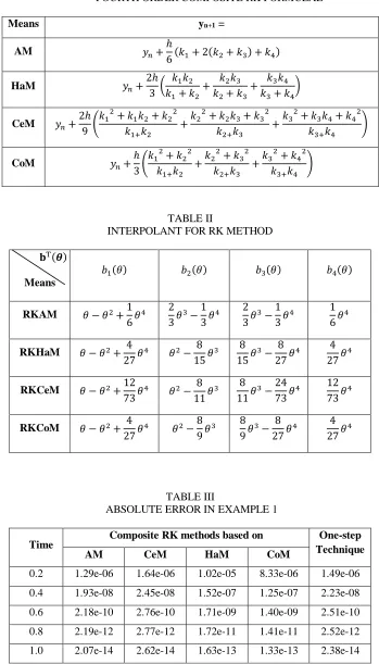
TABLE I

FOURTH ORDER COMPOSITE RK FORMULAE

Means yn+1 =

AM 𝑦𝑛+

ℎ

6(𝑘1+ 2(𝑘2+ 𝑘3) + 𝑘4)

HaM 𝑦𝑛+

2ℎ 3 (

𝑘1𝑘2

𝑘1+ 𝑘2

+ 𝑘2𝑘3 𝑘2+ 𝑘3

+ 𝑘3𝑘4 𝑘3+ 𝑘4

)

CeM 𝑦𝑛+

2ℎ 9 (

𝑘12+ 𝑘1𝑘2+ 𝑘22

𝑘1+𝑘2

+𝑘2

2

+ 𝑘2𝑘3+ 𝑘32

𝑘2+𝑘3

+𝑘3

2

+ 𝑘3𝑘4+ 𝑘42

𝑘3+𝑘4

)

CoM 𝑦𝑛+

ℎ 3(

𝑘12+ 𝑘22

𝑘1+𝑘2

+𝑘2

2_{+ 𝑘}

32

𝑘2+𝑘3

+𝑘3

2_{+ 𝑘}

42

𝑘3+𝑘4

)

TABLE II

INTERPOLANT FOR RK METHOD

𝐛T_(𝜽)

Means

𝑏1(𝜃) 𝑏2(𝜃) 𝑏3(𝜃) 𝑏4(𝜃)

RKAM 𝜃 − 𝜃2₊1

6𝜃

4 2

3𝜃

3₋1

3𝜃

4 2

3𝜃

3₋1

3𝜃

4 1

6𝜃

4

RKHaM 𝜃 − 𝜃2₊ 4

27𝜃

4 _𝜃2₋ 8

15𝜃

3 8

15𝜃

3₋ 8

27𝜃

4 4

27𝜃

4

RKCeM 𝜃 − 𝜃2₊12

73𝜃

4 _𝜃2₋ 8

11𝜃

3 8

11𝜃

3₋24

73𝜃

4 12

73𝜃

4

RKCoM 𝜃 − 𝜃2₊ 4

27𝜃

4 _𝜃2₋8

9𝜃

3 8

9𝜃

3₋ 8

27𝜃

4 4

27𝜃

4

TABLE III

ABSOLUTE ERROR IN EXAMPLE 1

Time Composite RK methods based on _Technique One-step

AM CeM HaM CoM

0.2 1.29e-06 1.64e-06 1.02e-05 8.33e-06 1.49e-06

0.4 1.93e-08 2.45e-08 1.52e-07 1.25e-07 2.23e-08

0.6 2.18e-10 2.76e-10 1.71e-09 1.40e-09 2.51e-10

0.8 2.19e-12 2.77e-12 1.72e-11 1.41e-11 2.52e-12

1.0 2.07e-14 2.62e-14 1.63e-13 1.33e-13 2.38e-14

IAENG International Journal of Applied Mathematics, 49:3, IJAM_49_3_14

[image:7.612.133.481.82.241.2] [image:7.612.131.482.97.377.2]

TABLE IV

ABSOLUTE ERRORS OF y1 IN EXAMPLE 2

TABLE V

ABSOLUTE ERRORS OF y2 IN EXAMPLE 2

TABLE V1

ABSOLUTE ERROR IN EXAMPLE 3

Time Composite RK methods based on _Technique One-step

AM CeM HaM CoM

0.2 5.22e-14 3.55e-13 1.39e-12 1.36e-12 4.74e-13

0.4 1.30e-13 6.05e-13 2.55e-12 2.42e-12 8.57e-13

0.6 2.23e-13 7.76e-13 3.50e-12 3.24e-12 1.16e-12

0.8 3.21e-13 8.84e-13 4.28e-12 3.86e-12 1.40e-12

1.0 2.24e-11 2.38e-11 1.79e-11 2.72e-11 1.59e-12

Time Composite RK methods based on _Technique One-step

AM CeM HaM CoM

0.2 9.45e-07 9.45e-07 9.45e-07 9.45e-07 8.95e-07

0.4 1.63e-06 1.63e-06 1.63e-06 1.63e-06 1.54e-06

0.6 2.11e-06 2.11e-06 2.11e-06 2.11e-06 1.99e-06

0.8 2.42e-06 2.42e-06 2.42e-06 2.42e-06 2.29e-06

1.0 2.62e-06 2.62e-06 2.62e-06 2.62e-06 1.85e-06

Time Composite RK methods based on Technique One-step

AM CeM HaM CoM

0.2 1.16e-07 2.46e-07 5.06e-07 2.03e-07 1.16e-07

0.4 1.39e-07 1.47e-07 1.14e-07 1.64e-07 1.39e-07

0.6 1.57e-07 1.67e-07 1.29e-07 1.86e-07 1.57e-07

0.8 1.69e-07 1.79e-07 1.40e-07 1.98e-07 1.69e-07

1.0 4.19e-05 2.34e-05 1.00e-05 1.24e-04 1.74e-07

IAENG International Journal of Applied Mathematics, 49:3, IJAM_49_3_14

Fig. 1 (RKAM)

Fig. 2 (RKCeM)

Fig. 3 (RKCoM)

IAENG International Journal of Applied Mathematics, 49:3, IJAM_49_3_14

[image:9.612.199.409.56.681.2]

[image:10.612.204.408.60.230.2]

Fig. 4 (RKHaM)

Fig. 5 Stability region of the new one-step technique

IAENG International Journal of Applied Mathematics, 49:3, IJAM_49_3_14

[image:10.612.202.407.62.431.2]