Kazuki Ota, Hideki Katagiri
Abstract—Recently, the demand for ultra-high definition with 4K and 8K panels has increased. The study in this paper develops a fast algorithm for detecting wiring defects of glass substrates, which is based on an analysis done on time series data obtained through non-contact electronic inspection. New feature quantities with respect to the frequency domain of time series data are proposed. To demonstrate the effectiveness of the proposed algorithm, numerical experiments are conducted using the real sensing data obtained in the field of glass substrate inspection.
Index Terms—defect detection, machine learning, glass sub-strate, time series data, non-contact inspection, frequency-domain feature
I. INTRODUCTION
R
ECENTLY, the flat panel industry such as liquid crystal and organic electro-luminescence has grown. This has led to an increase in the demand for ultra-high definition with 4K and 8K panels. Increasing products yield rate reduces the unit price of products while improving productivity. Therefore, the wiring inspection of glass substrates is one of the most crucial processes. Hence, recently, the conduction test of wiring is performed in the middle process. Thereafter, detected defects are easily and certainly repaired to improve the product yield rate.In recent years, the non-contact continuity test of wiring in the middle process has attracted attention. In non-contact electrical inspection, the presence or absence and location of wiring defects are identified by analyzing the change in time series data of minute voltage obtained by scanning glass substrates with on inspection jig.
It is necessary that the defect detection of glass substrates from the inspection field is performed in real time without giving an erroneous detection. When defects are detected in the inspection process, it is necessary to capture an image of the defect after moving the camera to the corresponding wiring defect. When noise is falsely detected as a defect, the camera cannot find the defect. Therefore, an error will appear, and the inspection system will stop. In addition, there are multiple steps in the production of glass substrates. Therefore, it is necessary to conduct a continuity inspection
Manuscript received July 20, 2019; revised July 30, 2019.
O. Kazuki is with Department of Industrial Management Engineer-ing, Graduate School of EngineerEngineer-ing, Kanagawa University, 3-27-1 Rokkakubashi, Kanagawa-ku, Yokohama-shi, Kanagawa 221-8686, Japan (e-mail: [email protected]).
H. Katagiri is with Department of Industrial Management and Engineering, Faculty of Engineering, Kanagawa University, 3-27-1 Rokkakubashi, Kanagawa-ku, Yokohama-shi, Kanagawa 221-8686, Japan (e-mail: [email protected]).
on the field in real time to avoid waiting during the later steps.
Although there are several studies in the field of anomaly detection for defect detection, these studies cannot be ap-plied, because it needs to be performed in real time.
There are several studies in the field of anomaly detec-tion for defect detecdetec-tion. The wavelet transform, Fourier transform, and state-space model are the techniques that are commonly used in this field [1], [2], [3], [4], [5], [6]. Although there are several techniques, this research needs to be done in real time and cannot be applied as it is.
In conventional research on contactless electrical inspec-tion, methods for discrimination using thresholds [7] and methods using machine learning [8] have been proposed [9]. Although various waveform types exist depending on the wiring spacing and the surface roughness of glass substrates, there have been several waveform types where noise is falsely detected as a defect by conventional studies [7], [9].
In this study, we propose new feature quantities focusing on the frequency domain of time series data obtained from non-contact electrical inspection of glass substrates and fast detect defection algorithm of glass substrates by machine learning. In addition, we compare data with several conven-tional methods using the real inspection data and verify the usefulness of the proposed method.
II. INSPECTION DATA ACQUISITION METHOD AND CONCEPT OF DEFECT DETECTION
This section describes glass substrates electrical inspec-tion and defect detecinspec-tion on glass substrates. Secinspec-tion II-A describes the method for non-contact inspection of glass substrates. The concept of finding defects from the obtained inspection data will be explained in Section II-B. Section II-C describes the effects of false detection in the detection of defects on glass substrates. Section II-D shows conventional research on defect detection of glass substrates.
A. Non-contact electrical inspection of glass substrates
As the wiring in glass substrates is a conductor such as aluminum or silver, the non-contact inspection can be contacted based on the principle of parallel plate capacitors. As shown in Fig. 1, time series data of minute voltages can be obtained by scanning glass substrates with the inspection jig.
Fig. 1. System configuration diagram of non-contact electric inspection([7])
Fig. 2. Waveforms obtained from non-contact electrical inspection
B. Defect detection from minute voltage data
If there are defects such as a wire break, the amplitudes of waveforms of part corresponding to defects are larger than the peripheral part in the time series data of minute voltage. The most basic idea of defect detection is to set a threshold as shown in Fig. 3, and subsequently then to determine the part whose voltage is over the threshold as a defect.
'HIHFWSDUW 7KUHVKROG
Fig. 3. Defect detection by setting a threshold
As shown in Fig. 4, it may be difficult to set an appropriate threshold. For example, in Fig. 4, the left part whose voltage is over the threshold is falsely detected as a defect although it is noise.
'HIHFWSDUW 1RLVHSDUW
7KUHVKROG
Fig. 4. Example of detection error
[image:2.595.54.286.170.261.2]In addition, as shown in Fig. 5, various types of inspection data with trend or periodicity can be obtained in the field of glass substrates inspection. Therefore, defects and noise cannot be determined correctly only by setting a threshold to the obtained data.
Fig. 5. Various waveform types of inspection data
C. The importance of suppressing false detection
One of the goals of this study is to reduce false detection in the electrical inspection of glass substrates. The reason for this is that if false detection occurs frequently, the inspection system will stop temporarily and the inspection efficiency would decrease. When defects are detected in the inspection process, it is necessary to capture an image of the defect after moving the camera to the corresponding wiring defect. When noise is falsely detected as a defect, the camera cannot find the defect. Therefore, an error will appear and the inspection system will stop, leading to a decrease in inspection efficiency.
D. Issues in conventional research
This section shows conventional research. First, II-D1 and II-D2 will describe research on defect detection using time series data obtained from contact electrical inspection. Finally, the studies on general defect detection are described in II-D3.
1) Defect detection method using the threshold:
Hamori et al. [7] proposed a method to detect defects by setting a threshold after repeating the following three steps: (1) difference value calculation, (2) minute change emphasis, and (3) spike noise smoothing. Their method is effective when compared to the basic idea presented in Section II-B. However, their method often misses a type of defects where the wiring is about to be cut. In addition, there are problems where their method is difficult to cope with various inspection data. Moreover, it is difficult for operators to set an appropriate thresholds through experience and trial-and-error.
2) Defect detection method using machine learning: Wakamatsu et al. [9] proposed a new defect detection algorithm to solve the problem of Hamori et al. [7]. It became possible to detect defects for various types of inspection data, including types with minor changes that could not be detected by the study of Hamori et al.. Wakamatsu et al. proposed a “trend removal by using moving average curve method”. Moreover, Wakamatsu et al. constructed a defect detection algorithm based on machine learning using newly proposed “Z score” and “Isolations” feature quantities to emphasize small changes.
[image:2.595.56.284.410.505.2] [image:2.595.53.288.598.686.2]such as the method of a state space model, and density ratio estimation, along with methods based on signal processing techniques such as empirical mode decomposition and sin-gular spectrum transformation. Although there are various conventional studies, these studies are computationally slow and cannot be applied directly to this study.
As one of the algorithms specialized for anomaly detec-tion, an isolation forest (IF) [10] based on ensemble learning using a decision tree has been proposed. In this study, we use it as a comparison method in the numerical experiments described later.
III. PROPOSED DEFECT DETECTION ALGORITHM
In this research, based on the problems of conventional research, we improve the trend removal methods and propose new feature quantities used for machine learning. Moreover, we propose an algorithm to detect defects of glass substrates wiring in real time with higher accuracy than the conven-tional method.
First, the details of the feature quantities used for trend removal will be described in Section III-B. Subsequently, the detail of trend removal algorithm is explained in Section III-C. Finally, the details of feature quantities and machine learning used for defect detection will be presented in section III-D.
A. Outline of proposed defect detection algorithm
The outline of the algorithm proposed in this study is as follows. At this time, Xt, t = 0,1,2, . . . , m is the voltage signal data obtained by non-contact electrical in-spection. Frequency domain G(k), k = 0,1,2, . . . , m−1 is obtained by applying a fast Fourier transform (FFT) to
Xt. Furthermore, the time series data after trend removal is Xt′, t = 0,1,2, . . . , m. Frequency domain G′(k), k = 0,1,2, . . . , m−1 is obtained by applying FFT to Xt′.
Step 1 Calculate the “number of trend change” fromXt. Step 2 From Xt, calculate the “average number of data
contained between peak points [9]”.
Step 3 Calculate the “crest factor of the frequency domain” from G(k).
Step 4 Do trend removal using feature quantities obtained in Steps 1, 2, and 3.
Step 5 Calculate the “Z score [9]” and the “Isolations [9]” from Xt′.
Step 6 Calculate the “Z score of the frequency domain” from G′(k).
Step 7 Machine-learned defect detection is performed us-ing the feature quantities obtained in Steps 5 and 6.
Steps 2 and 5 are almost the same as in the conventional research [9]. Hence, the explanations of these steps have been omitted.
domain” in III-B2 to improve the trend removal method.
1) Number of trend changes(Tr):
The details of Step 1 in the defect detection algorithm shown in Section III-A are given below.
As shown in Fig. 5, it can be seen that the frequency, presence or absence of the trend, and the number of changes in the trend differ depending on waveform types. It is possible to identify the difference in frequency by the “av-erage number of data between extremes” and “proportion of extremes” proposed in the previous research.
However, the previous research by Wakamatsu et al. [9] was not able to identify the trend and the number of changes. Therefore, in this study, we propose the “number of trend changes” that calculates the change from rising to falling or the opposite of the waveform that occurs.
The details of Step 1 in the defect detection algorithm shown in Section III-A are given below.
Step 1-1 The exponential smooth moving average St(θ) of the time series data Xt of the minute voltage signal is calculated by Eq. (1).
St(θ) =θXt−1+ (1−θ)St−1(θ), (1)
whereθis an exponential smoothing parameter that satisfies0≤θ≤1 andS1(θ) =X1.
Step 1-2 The difference between the exponential smooth moving average for two different exponential smoothing parameters is calculated using Eq. (2).
DSt(θ, θ′) =St(θ)−St(θ′), (2)
whereθandθ′ are exponential smoothing parame-ters.
Step 1-3 The exponential smooth moving average
Ut(θ, θ′, θ′′)ofDSt(θ, θ′)is calculated by Eq.(3).
Ut(θ, θ′, θ′′) = θ′′DSt−1(θ, θ′)
+ (1−θ′′)Ut−1(θ, θ′, θ′′), (3)
where θ, θ′ and θ′′ are exponential smoothing parameters, andU1(α) =DS1(θ, θ′).
Step 1-4 Calculate Eq.(4).
ST r0 ={t|DSt(θ, θ′)−Ut(θ, θ′, θ′′) = 0}
and
T r=|ST r0|, (4)
where|ST r0|represents the number of elements in the setST r0.
DSt(θ, θ′)calculated in Step 1-2 is an approximate shape of the trend for the original dataXt (See Fig. 6).
2ULJLQDO'DWD
[image:4.595.52.282.51.157.2]࢚, ᇱ
Fig. 6. Computation in Step 1-2
number of times the trend switches is calculated by counting the intersection ofDSt(θ, θ′)andUt(θ, θ′, θ′′).
࢚, ᇱ
[image:4.595.314.540.52.194.2]࢚, ᇱ, ᇱᇱ
Fig. 7. Trend changing points
2) Crest factor of frequency domain(crf)[11]:
The details of Step 3 in the defect detection algorithm shown in Section III-A are given below.
To properly perform the trend removal method, it is necessary to consider not only the time domain but also the features of the frequency domain. In conventional research [9], feature quantities in the time domain were proposed. In addition, the “number of trend change” proposed as a new feature quantity in section III-B1 is also a time domain feature quantity.
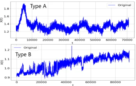
First, the necessity of the feature quantities based on the frequency spectrum is explained. In Fig. 8, the number of trend change in the two waveforms is almost equal. While the wave component of the specific cycle is seen in waveform Type A, the wave component having various cycle is mixed in the waveform Type B. Therefore, it is necessary to make the average interval value smaller for Type B when compared to Type A. However, if only the number of trend changes is used as the feature quantity trend removal cannot work properly, because the move average interval values of Types A and B are almost equal.
Based on the above-mentioned considerations, the details of Step 3 in the defect detection algorithm shown in Section III-A are as follows.
Step 3-1 For Xt, calculate the frequency spectrum G(k) by FFT.
Step 3-2 The crest factor ofG(k)is calculated by Eq. (5).
crf =G(k)max
G(k)real
, (5)
whereG(k)maxandG(k)realare the maximum and
effective values ofG(k), respectively, and they are
7\SH $
7\SH%
Fig. 8. Two inspection data having almost equal number of trend changing points
defined by the following equations.
G(k)max = max
k=1,...,m−1G(k),
G(k)real =
v u u
t 1
m−1
m∑−1
i=0
G(i)2.
In Step 3-1, the frequency spectrum is calculated by FTT for minute voltage signal data (See Fig. 9).
7\SH $
7\SH%
Fig. 9. Frequency spectrum of two inspection data
The crest factor calculated in Step 3-2 represents the sharpness of the maximum value in the frequency spectrum. The higher this feature quantity, the stronger is the influence of the wave component of the specific cycle. In Fig. 7, the crest factor of Type A is larger than that of Type B.
C. Trend removal algorithm
In this research, we consider a new trend removal method using the trend change number and the crest factor of the frequency component proposed by Eqs (4) and (5). The details of Step 4 in the defect detection algorithm shown in Section III-A are as follows.
Step 4-1 Calculate the move average interval values
[image:4.595.51.284.238.345.2] [image:4.595.310.539.381.532.2]interval values obtained in Step 4-1.
Step 4-3 The absolute values of the difference between the original data and its move average curve are calculated, and the top peak point is extracted to obtain time series data.
Step 4-4 Calculate the move average curve of time series data obtained in Step 4-3. Repeat the steps from Step 4-1 to Step 4-4η times.
D. Feature quantities and machine learning algorithms used for defect detection
The details of Steps 6 and 7 in the defect detection algorithms shown in Section III-A are given below.
Step 6-1 ForXt′, calculate the frequency spectrumG′(k) by FFT.
Step 6-2 Calculate the Z score ofG′(k) obtained in Step 6-1.
F(k) =G
′(k)−µ
σ , (6)
where µ and σ represent the mean and standard deviation ofG′(k), respectively.
There are three feature quantities used for machine learn-ing in Step 7 of the defect detection algorithm shown in Section III-A. The first and second are the “Z score” and the “Isolations” of Xt obtained in Step 5 of Section III-A.
The third is F(k) obtained in Step 4 of Section III-A. In this study, we investigate a support vector machine (SVM), the k-nearest neighbor method (k-NN), gradient boosting (XGBoost), the random forest (RF), and the isolation forest (IF).
IV. EXPERIMENT
We confirm the effectiveness of the proposed method in this research. The actual data (238 waveform data) obtained from the field of the inspection process of glass substrates were used for the experiment. The values of parameters were
θ = 0.016, θ′ = 0.007, θ′′ = 0.021, α= 0.90, β = 0.50,
γ= 0.90,η= 3.
The programming language used for implementation is Python 3.65, and the operating environment is CPU: Core i5-6400, RAM: 16.0 GB, OS: Windows 10. For machine learning programs, we used the Python libraries scikit-learn ver. 0.201 and XGBoost ver. 0.81.
The total inspection data was 495.16 s, and about 2.08 s per waveform data until the calculation of the feature quantities used for machine learning was completed.
TABLE I
COMPARISON OF PERFORMANCE OF THE PREVIOUS ALGORITHM[7]AND THE PROPOSED ALGORITHM
Threshold defect detection[7] k-NN Threshold 4.0×10⁻⁵ 8.0×10⁻⁵ 1.2×10⁻⁶ 1.6×10⁻⁶ 2.0×10⁻⁶ True Positive Rate(%) 91.0 84.6 82.9 80.2 79.1 81.4 False Negative Rate(%) 70.5 63.9 60.9 58.8 56.9 5.09×10⁻⁵
As listed in Table I, with the conventional method of Hamori et al. [7], the True Positive Rate is high at any threshold, and defects can be detected with high accuracy. In contrast, the false positive rate is as high as approximately 60%. Therefore, in several cases, noises are falsely detected as defects.
When the threshold is set to1.2×10−6 and1.6×10−6, although the True Positive Rate of the conventional method is equal tok-NN, there is a large difference in False Positive Rates. The proposed method is shown to be an excellent method to detect defects with high accuracy while minimiz-ing false detection.
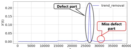
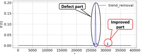
B. A comparative experiment on the trend removal method When the conventional trend removal method was applied, the defects in 22 waveforms out of 238 waveform data could not be detected. In contrast, applying the detrending method proposed in this research could reduce 22 waveforms to 9 waveforms. An example of the improvement is shown in Fig. 10 below.
[image:5.595.314.539.497.586.2]'HIHFWSDUW
Fig. 10. Example of data containing defects
'HIHFWSDUW
0LVVGHIHFW SDUW
Fig. 11. Result of trend removal by the previous study[9]
[image:5.595.312.539.635.721.2]'HIHFWSDUW
[image:6.595.57.283.53.139.2],PSURYHG SDUW
Fig. 12. Result of trend removal by the proposed method
research was used (See Fig. 11), the change corresponding to the defect on the right was small and could not be detected as a defect. However, in the proposed trend removal method (See Fig. 12), the change corresponding to the defect on the right side became clear and could be detected correctly as a defect.
C. Experiment on Machine Learning Algorithm and Influ-ence of Parameters
In this study, hyperparameters of machine learning algo-rithms such as SVM, XGBoost, RF, and IF are set to be default values of the Python libraries scikit-learn ver. 0.201 and XGBoost ver. 0.81. We use four evaluation metrics: (1) Accuracy, (2) Precision, (3) Recall, and (4) F-measure. In addition, we examined the validity of the model using cross validation with a division number of 9.
1) Comparison result of machine learning algorithm: Table II shows the comparison results of applying the machine learning algorithm. Notably,k= 13is set fork-NN.
TABLE II
PERFORMANCE COMPARISON OF DIFFERENT MACHINE-LEARNING ALGORITHMS
SVM XGBoost RF IF k-NN Accuracy(%) 99.9 99.9 99.9 99.9 99.9
Precision(%) 87.4 79.1 50.4 0.4 90.4
Recall(%) 79.8 76.2 82.1 100 81.4 F-measure(%) 79.5 78.0 77.1 0.8 82.4
As listed in Table II, the Accuracy, Precision, and Recall of k-NN (k = 13) are well-balanced compared to other methods, and the F-measure, which is the overall judgment index, is the highest.
2) Parameter setting in k-nearest neighbor method: Table III lists the results when the value ofkis changed in order to investigate the influence of the value of k onk-NN.
TABLE III
PERFORMANCE COMPARISON OFk-NNWITH DIFFERENT PARAMETERk
k= 1 k= 3 k= 5 k= 7 k= 9 k= 11 k= 13 k= 15 Accuracy(%) 99.9 99.9 99.9 99.9 99.9 99.9 99.9 99.9 Precision(%) 76.2 82.0 86.2 88.4 88.4 89.1 90.4 89.6 Recall(%) 80.0 81.4 80.0 81.4 82.1 82.1 81.4 80.7 F-measure(%) 78.6 83.2 83.0 84.6 82.1 82.4 82.4 84.6
In Table III, judging from the F value, the best results were obtained when k= 11,13. In addition, except for the case of settingk= 1, the F-measure is stable above 83% in
all cases, and the proposed method shows desirable results from the viewpoint of robustness.
V. CONCLUSION
In this research, we have proposed feature quantities of frequency components and the trend removal method based on a new move average interval value calculation method. Furthermore, we have constructed a fault detection method based on machine learning. In addition, experiments were conducted using glass substrate inspection data of the field. Moreover, performances were compared by applying mul-tiple machine learning algorithms. The experimental results show that thek-nearest neighbor method is excellent not only in detecting defects on glass substrates with higher accuracy than conventional methods [7] but also in the inspection field in terms of improving inspection efficiency.
As future work, we will verify the effectiveness of the proposed method using additional inspection field data. In addition, we will consider the proposal of a new feature quantities and trend removal algorithm using frequency com-ponents to further enhance defect detection accuracy.
ACKNOWLEDGMENT
We would like to thank Dr. Hiroshi Hamori, President and CEO of HTC Co., Ltd., for providing the glass substrate inspection data in carrying out this research. In addition, in carrying out this research, Makoto Mitsuishi (Kanagawa University, 2019, Now Fujitsu Ltd.) conducted many use-ful discussions and computer experiments. We express our gratitude to them.
REFERENCES
[1] C. Li, R. V. Sanchez, G. Zurita, M. Cerrada, and D. Cabrera, “Fault diagnosis for rotating machinery using vibration measurement deep statistical feature learning,”MDPI, vol. 16, no. 6, p. 895, 2016. [2] B. Li, M.Y. Chow, Y. Tipsuwan, J.C. Hung, “Neural-network-based
motor rolling bearing fault diagnosis,”IEEE Transactions on Industrial Electronics, vol. 47, no. 5, pp. 1060–1069, 2000.
[3] Zhiwei Gao, Carlo Cecati, Steven X. Ding, “A survey of fault diagnosis and fault-tolerant techniques - part 1: Fault diagnosis with model-based and signal-model-based approaches,”IEEE Transactions on Industrial Electronics, vol. 62, no. 6, pp. 3757–3767, 2015.
[4] Hai Qiua, Jay Leea, Jing Linb, Gang Yu, “Wavelet filter-based weak signature detection method and its application on rolling element bearing prognostics,”Journal of Sound and Vibration, vol. 289, no. 4–5, pp. 1066–1090, 2006.
[5] H.A. Toliyat, K. Abbaszadeh, M.M. Rahimian, L.E. Olson, “Rail defect diagnosis using wavelet packet decomposition,”IEEE Trans-actions on Industry Applications, vol. 39, no. 5, pp. 1454–1461, 2003. [6] A. Abbate, J. Koay, J. Frankel, S.C. Schroeder, P. Das, “Signal detection and noise suppression using a wavelet transform signal pro-cessor: Application to ultrasonic flaw detection,”IEEE Transactions on Ultrasonics, Ferroelectrics, and Frequency Control, vol. 44, no. 1, pp. 14–26, 1997.
[7] H. Hamori, M. Sakawa, H. Katagiri, and T. Matsui, “Fast non-contact flat panel inspection through a dual channel measurement system,” in The 40th International Conference on Computers & Indutrial Engineering, 2010, pp. 1–6.
[8] R. T. T. Hastie and J. Friedma,The Elements of Statistical Learning. Springer, 2009.
[9] R. Wakamatsu, T. Uno, and H. Katagiri, “Machine learning-based methods for detecting defects in glass substrate from non-contact electrical sensor data,” inWorld Congress on Engineering 2018, vol. 1, 2018.
[10] F. T. Liu, K. M. Ting, and Z.-H. Zhou, “Isolation forest,” in2008 8th IEEE International Conference on Data Mining, 2008, pp. 413–422. [11] B. Sreejith, A. Verma, and A. Srividya, “Fault diagnosis of rolling
element bearing using time-domain features and neural networks,” in
![Fig. 1. System configuration diagram of non-contact electric inspection([7])](https://thumb-us.123doks.com/thumbv2/123dok_us/392534.536793/2.595.53.288.598.686/fig-conguration-diagram-non-contact-electric-inspection.webp)