Online Full Text



Abstract— A high number of IT organizations have problems when deploying their services, this alongside with the high number of services that organizations have daily, makes Incident Management (IM) process quite demanding. An effective IM system need to enable decision makers to detect problems easily otherwise the organizations can face unscheduled system downtime and/or unplanned costs. By predicting these problems, the decision makers can better allocate resources and mitigate costs. Therefore, this research aims to help predicting those problems by looking at the history of past deployments and incident ticket creation and relate them by using machine learning algorithms to predict the number of incidents of a certain deployment. This research aims to analyze the results with the most used algorithms found in the literature.

Index Terms—Predictive Analysis, Incident Management, Software Deployment, Machine Learning

I. INTRODUCTION

HOUSANDS of IT organizations worldwide are struggling with the deployment of IT service management processes (ITSM) by having problems deploying the service into the daily IT operations [1] this alongside with a high number of services, different types of organization and a huge growth in IT make IT service managers be under pressure to reduce costs and quickly deliver cost effective services [2] and consequently makes Incident Management (IM) process quite demanding.

Nowadays, many tickets are created each day [3], especially in large-scale enterprise systems [4], [5]. A recent study from [6] reported that about 12 billion lines of log messages are generated in their infrastructure each day for IM and most of these tickets are created with non-structured text [5] meaning that they can have numerous variations on the description of it and organizations are not able to extract value from such data.

Manuscript received March 2019; revised April 2019. This work has been partially supported by Portuguese National funds through FITEC - Programa Interface, with reference CIT "Inov - Inesc Inovação - Financiamento Base",

Jose Messejana is with Instituto Universitário de Lisboa (ISCTE-IUL), Av. das Forças Armadas, 1649-026 Lisboa, Portgual phone: +351210464277; (e-mail:[email protected]).

Ruben Pereira is with Instituto Universitário de Lisboa (ISCTE-IUL), ISTAR-IUL (e-mail: [email protected])

Joao C. Ferreira is with Instituto Universitário de Lisboa (ISCTE-IUL), ISTAR-IUL and Inov - Inesc Inovação (e-mail: [email protected])

Marcia Baptista is with Inov - Inesc Inovação (e-mail: [email protected]).

An effective IM system needs to enable decision makers to detect anomalies and extract helpful knowledge to solve incidents [2]. These incidents can lead to unscheduled system downtime and/or unplanned costs [7] and cause a huge impact since the recovery process can require time and resources that were not considered [8]. Furthermore, if administrators can predict these incidents, they can better allocate their resources and services to mitigate the costs [7]. Accurate failure predictions can help in mitigating the impact of computer failures even when the failure is impossible to solve, because recovery and rescue can be taken way earlier [9] and allow managers to get a better response over system performance [7].

This is where Predictive Analysis can help predicting future incidents by using retrospective and current data [10]. In recent years, machine learning, as an evolving subfield of computer science has been widely used on the challenging problem of incidents and anomaly detection problems [11] and can nowadays provide information on the applications and the environments where the applications are deployed [12].

As previously stated, there is a huge number of incidents reported each day, making it difficult for organizations to keep up with it and a possible solution would be using predictive analysis to predict some of those incidents and therefore reduce those incidents and the possible costs associated with them.

Software deployments can have critical information to predict and therefore prevent incidents, like a feature that often causes many incidents when there is a deployment with it, and so this research aims to analyze several software deployments of the last few years and make a match with the incidents reported in the same period to build a predictive model capable of predicting and understand incidents based on the deployments to be made.

II. RELATED WORK

This section provides a critical analysis about what has been done that relates to this study. Although there are some studies using the source code and repository information, such as commits to predict incidents, there was nothing found using deployment information similar to what this research will use. Because of that, this section will gather some of those studies that study software fault predictions with code inspection and then gather the studies that use machine learning algorithms to predict incidents based on some sort of textual information.

The authors from [13] did systematic literature review software fault prediction metrics of 106 studies to determine what are the software metrics that contribute the most to the

Jose Messejana, Ruben Pereira, Joao C Ferreira, and Marcia Baptista

Predictive Analysis of Incidents based on

Software Deployments

software failure. This research focused on code inspection, code history, context, software development lifecycle and person who develop the code. Another study that used code inspection to predict incidents was [14], that focus on using symbolic analysis on python code to predict possible failures. The authors from [15] studied the relation between system logs and code quality.

A. Mukhopadhyay [16] researched 90 papers trough 1990 to 2009, like the previous research all these papers used code inspection metrics to predict failures. The most used algorithms found here were Classification and Regression Trees (CART) (in the early years), logistic regression and Naïve Bayes.

In [7] used Support Vector Machine (SVM) to encode the execution logs into features readable by it by using for example text mining since log messages are often in free-format text. The authors then refer that the authors from [15], [17] divided static from dynamic information in logs and combined sequences by their dynamic information to standardize them.

The authors from [18] the recall and file inspection ratio were used to validate the predictions and it was said that vulnerability predictions favour high recall. The classifiers were evaluated using Monte-Carlo simulations for different values of their internal parameters and simulation results are assessed with precision, recall, accuracy and f-measure.

In the study from [19] the objective was to compare Neural Networks (NN), CART and non-linear regression algorithms using a dataset of smokers containing mostly categorical values by comparing the errors from the predictions where the predictor values are categorical, and the known variables are all continuous. They concluded that NN and CART clearly produced better results than non-linear regression. It was reported that Decision Trees (DT) based models (like CART) can scale up to large problems and can handle smaller data sets better than NN. Despite that performed better on large data sets but with a low number of attributes.

G. Tziroglou [11] research made a comparison between SVM, DT, logistic regression and Naïve Bayes to predict industrial incidents by using temperature and time attributes and by evaluating them in the end trough cross validation using 100 Monte-Carlo iterations (to reduce the bias) dividing 70% for training and 30% for testing and by applying Adaptive Boost in the SVM and DT algorithms. After analyzing the data, they decided to label the classes in two categories depending on the actual and desired temperature and a threshold for the difference of the two. In the end the authors concluded that SVM with adaptive boost had the best results with 98% accuracy and 97% F-measure. The cross-validation used by the authors was custom made, since the regular cross-validation divides the dataset into k parts, but here the author started by doing set split and then used Monte-Carlo to reduce bias like they state in the re-search, but they do not say why they did not use the regular cross-validation technique that aims to also reduce the bias [20].

S. Kikuchi [4] research aimed to predict the workload of incident tickets, to do that the author made an analysis on incident tickets that might be useful to this research. The

author said that the time that a ticket takes to be closed does not represent difficulty or amount of workload. The author ended up using status updates to replace the time. The difficulty was then categorized into easy and difficult incidents based on the number of updates. To predict and evaluate, it was used TF-IDF to relate the ticket descriptions categorizing each ticket in easy or difficult and then using Naïve Bayes for clustering. To validate the results the author split the dataset 75%-25% (training-test).

Like it was said on the beginning of this chapter there was not any study using deployment information, so this research aims to fill that gap.

III. WORK METHODOLOGY

The research methodology used in this research will be the Cross Industry Standard Process for Data Mining (CRISP-DM). This methodology aims to create a precise process model for data mining projects [21].

This methodology has six different phases. These phases include [22]:

• Business Understanding - the objective is to

understand the requirements and objectives of a project and turn that into a data mining problem.

• Data Understanding – This phase is a

complementation of the previous one as to understand the data, one needs to understand the context in which they will be used and to understand the objective of the project, one must know what the type of data that will be used.

• Data Preparation - After a good understand of the

business and data, data preparation can start. This phase is the combination of all the necessary activities to build the final dataset which include attribute selection, data cleaning, construction of new attributes and data transformation.

• Modelling - As this aims to apply different modelling

techniques and parameter calibration, this phase must be done back and forth with the previous one.

• Evaluation - After having one or two high quality

models by using data analysis, it is needed to do an evaluation of the model to prove that it can achieve the objectives proposed. To do this, the model will be assessed by using the most used metrics in the literature such as precision, recall, accuracy and f-measure.

• Deployment - the knowledge obtained in the model

needs to be presented trough a report or presentation or both.

IV. BUSINESS AND DATA UNDERSTANDING

The data used for this research was from a company operating in the bank sector in Portugal (only information possible to reveal due to privacy agreement) and consisted in two excels, one with deployment tickets information and the other with incident tickets information, such as date of end and start of the ticket, description, who made the deployment, where was the deployment assigned, different categories of the application or software.

114146 entries and 161 attributes.

Unfortunately, the dataset did not contain information that links an incident directly to a deployment. The description given in the incident tickets is not enough to know what may have been the deployment that caused it and so the only way to relate them is by the name of the application or software.

Table I and Table II show the top value for each dataset in a specific attribute.

The detailed description average length is 184 characters. The value of both Operational Categorization Tier 2 attributes in both tables are not the real ones for privacy reasons.

V. DATA PREPARATION

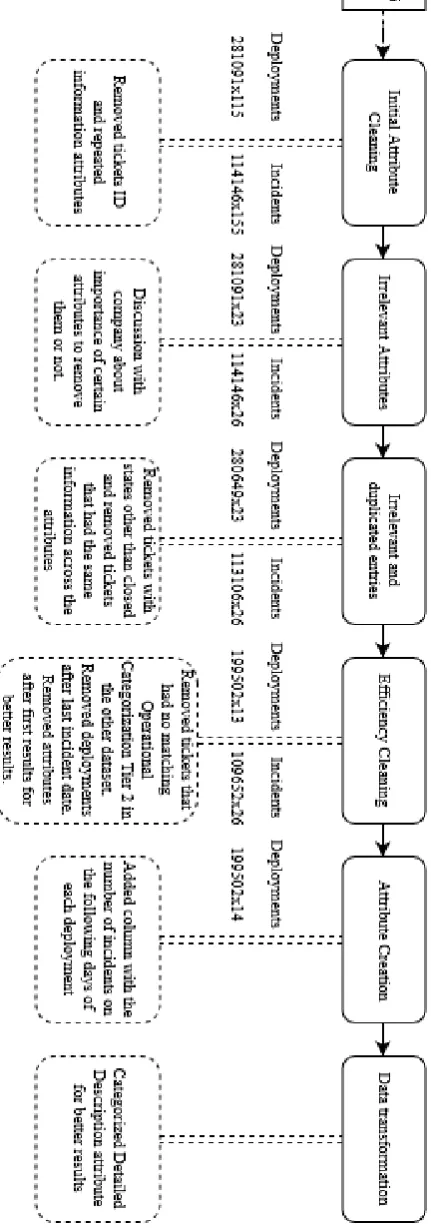
To achieve better results and to remove not necessary entries and attributes, several transformations were made before having the final dataset. Fig. 1 shows the workflow of the transformations, which will then be further explained throughout this chapter.

Fig. 1. Data preparation workflow TABLEI

DEPLOYMENTS ANALYSIS

Attribute Value Occurrences

Operational

Categorization Tier 2 Application X 96189

Operational Categorization Tier 1

Software/Applications

– Production 175927

Operational Categorization Tier 3

Request for analysis /

Clarification 22329

Completed Date 12th _{July 2017 406}

TABLEII INCIDENTS ANALYSIS

Attribute Value Occurrences

Operational

Categorization Tier 2 Application Y 14058

Operational Categorization Tier 1

Software/Applications

– Production 71786

Operational

Categorization Tier 3 Anomaly 31372

A. Initial Attribute Cleaning

After the first analysis it was taken out attributes that did not have any relevant information such as ticket ID and attributes that had repeated information of other attributes. 11 attributes from deployments and 6 from incidents were removed in this process.

B. Irrelevant attributes

Then after checking with the company to validate the relevance of some attributes, it was decided to eliminate more attributes such as attributes that most of the entries were empty and others, such as email, phone number, breach reason, model/version and many others that both the company and the authors agreed that would not bring much information.

After this the files went from 115 attributes to 23 in the deployment’s dataset and from 155 attributes to 26 in the incident’s dataset. In this process the start date of the deployments and the end date of the incidents were removed as they would not be needed because the intention is to relate when the deployment was made, and the incident was created.

C. Irrelevant and duplicated entries

After this, it was removed tickets entries with states other than closed to avoid having repeated tickets with only different states due to the dataset having different entries for the different states of the ticket and in the end the duplicates entries were removed.

442 entries from deployments and 1040 from incidents were removed in this process, leaving the dataset with 280649 entries in the deployment’s dataset and 113106 in the incident’s dataset.

D. Efficiency Cleaning

Then for efficiency purposes, it was removed the entries which didn’t have a match in the other excel making the deployment data going from 280649 entries to 199776 and the incident data from 113106 to 109652. The deployment dataset had deployments after the last incident date making them not useful, so these were removed, there were 274 deployment in this situation leaving the final deployment’s dataset with 199502. After the first results the authors decided to remove more attributes to see if it would make the algorithm have better results and so ten more attributes were removed leaving the deployments dataset with 13 attributes.

E. Attribute Creation

To make it possible to make a prediction it was needed to add an attribute that had the number of incidents of a deployment in the following days (for this research we used 3, 7 and 10 days), leaving the deployment dataset with 14 attributes.

F. Data transformation

The description attribute had all sort of information on it, so the authors decided to categorize it based on the size of the text by comparing them with the average field size. In the end, the attribute was divided in short, medium and long description and none.

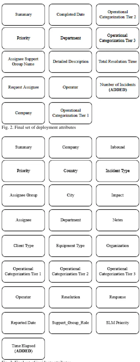
Fig. 2 shows the final set of attributes used from the deployment’s dataset. Fig. 3 shows the final set of attributes present in the incident’s dataset.

Fig. 2. Final set of deployment attributes

Fig. 3. Final set of incidents attributes

VI. MODELING

Following what was done in the previous section, the authors decided to apply Naïve Bayes and SVMto measure the accuracy of the prediction. The algorithms were used with the library sklearn in python with a validation size of 25% and 7 as seed. For the library to use the algorithm all data could not have any fields of type String or be empty, so the empty fields were filled with zeros and the strings were categorized by using a function from the same library. The algorithm was applied to the deployment file by trying to predict the number of incidents attributes that were created based on the comparison of the two datasets.

VII. EVALUATION

When the number of incidents were not categorized, the number of incidents had the following distribution, as showed in Table III.

As it can be seen there is a big distribution of values, so the authors decided to make different types of predictions.

 First, where the number of categories is zero meaning that the algorithm tries to predict exactly the number of incidents.

 Second, where the number of incidents is categorized in “no accidents” and “accidents”.

 Third in “no accidents”, “below average accidents” and “above average accidents”.

 Finally, in “no accidents”, “residual accidents” (one or two), “below average accidents” and “above average accidents”.

After applying the Naïve Bayes and SVM algorithms the results were the ones present in Table IV.

To evaluate the results the authors used accuracy,

precision, recall and measure. The precision recall and f-measure are the weighted average of each category meaning it considers the number of samples of each category.

 Accuracy - represents the ratio of correct predictions by the total number of predictions [23].

 Precision – Number of correct results divided by the number of guesses [23].

 Recall – Number of values that were supposed to be guessed and were guessed [23].

 F-Measure – Relates precision with recall by doing a weighted harmonic mean between them [23].

Both algorithms have similar results, although SVM has slightly better precision and slightly worse recall than Naïve Bayes.

VIII. CONCLUSION

As shown in the previous chapter, the best result came from Naïve Bayes with 82.7% when setting the number of incidents over 10 days and by categorizing them in no accidents and accidents. This does not allow to differentiate a deployment with 1 or 2 incidents from one with 100 incidents but allows us to predict with confidence if a deployment will or will not have a deployment.

In most cases the Naïve Bayes algorithm worked slightly better than SVM. The only time where this was not true was when there was not any categorization of the incidents. This might be due to the fact that SVM works better when there are few entries for a certain number of incidents, possibly relating the attributes better to each number of incidents, while Naïve Bayes goes more for a statistic approach, which ends up being worse if there are few examples for each category.

There is only a small difference in accuracy between 7 and 10 days, although with 10 days is slightly better. The prediction by using only 3 days of incidents had lower results, which can indicate that most of the incidents are not detected within this time, although this can be highly affected by the fact that weekends and holidays are not being considered.

TABLEIV ALGORITHM RESULTS

Number of categories Days

Accuracy (%) Precision (%) Recall (%) F-Measure (%)

Naïve Bayes SVM Naïve Bayes SVM Naïve Bayes SVM Naïve Bayes SVM

0

3 22.9 24.3 12 24 23 24 23 10

7 15.4 15 6 22 15 15 8 4

10 13.1 13 5 25 13 13 6 3

2

3 69.8 62.7 68 66 70 63 68 49

7 80.5 79 79 82 81 79 79 70

10 82.7 82.7 81 86 83 73 82 75

3

3 58.9 52.7 53 57 59 53 54 37

7 62.3 60 57 69 62 60 57 45

10 62.5 60.4 56 72 61 60 55 46

4

3 43.8 31.7 38 48 44 32 36 16

7 56.1 49 51 63 56 49 51 33

10 56.2 52.2 51 70 56 52 51 36

TABLEIII

NUMBER OF INCIDENTS DISTRIBUTION

Days Min Max Average Standard Deviation

3 0 562 9.1 20.2

7 0 648 19.9 37.3

Overall and despite not having any way to associate an incident directly to a deployment and not having detailed information on what was changed in the deployments the results still allow us to predict if a certain type of deployment with certain types of attributes has a high or low probability of having incidents, by raising aware of the deployment team to be more careful when doing the deployment. Although it does not have a high accuracy on guessing the exact number of incidents, it does have a good accuracy when deciding if a certain deployment has or not a incident and even when predicting if it will have just a few or around the average incidents which allows once again the deployer to have a better trust when deploying the application or software.

IX. FUTURE RESEARCH

Despite the interesting results already achieved, the authors are currently evolving this investigation by applying more algorithms such as Random Forest and CART. Other attributes are also being correlated, like severity of the incident, holidays, different days for the number of incidents attribute and by grouping up deployments made on the same day

ACKNOWLEDGMENT

This work has been partially supported by Portuguese National funds through FITEC - Programa Interface, with reference CIT "INOV - INESC INOVAÇÃO - Financiamento Base"

REFERENCES

[1] M. Jäntti and J. Järvinen, “Improving the Deployment of IT Service Management Processes: A Case Study,” in Systems, Software and

Service Process Improvement, vol. 172, R. V. O‘Connor, J.

Pries-Heje, and R. Messnarz, Eds. Berlin, Heidelberg: Springer Berlin Heidelberg, 2011, pp. 37–48.

[2] J. F. F. Aguiar, R. Pereira, J. B. Vasconcelos, and I. Bianchi, “An Overlapless Incident Management Maturity Model for Multi-Framework Assessment (ITIL, COBIT, CMMI-SVC),” Interdiscip.

J. Inf. Knowl. Manag., vol. 13, pp. 137–163, 2018.

[3] T. D. F. de Mello and E. C. Lopes, “Using case-based reasoning into a decision support methodology for the incident resolution control in IT,” in 2015 10th Iberian Conference on Information

Systems and Technologies (CISTI), 2015, pp. 1–6.

[4] S. Kikuchi, “Prediction of Workloads in Incident Management Based on Incident Ticket Updating History,” p. 8, 2015.

[5] D. Lin, R. Raghu, V. Ramamurthy, J. Yu, R. Radhakrishnan, and J. Fernandez, “Unveiling clusters of events for alert and incident management in large-scale enterprise it,” in Proceedings of the 20th ACM SIGKDD international conference on Knowledge discovery

and data mining - KDD ’14, New York, New York, USA, 2014, pp.

1630–1639.

[6] J.-G. Lou, Q. Lin, R. Ding, Q. Fu, D. Zhang, and T. Xie, “Experience report on applying software analytics in incident management of online service,” Autom. Softw. Eng., vol. 24, no. 4, pp. 905–941, Dec. 2017.

[7] B. Russo, G. Succi, and W. Pedrycz, “Mining system logs to learn error predictors: a case study of a telemetry system,” Empir. Softw. Eng., vol. 20, no. 4, pp. 879–927, Aug. 2015.

[8] E. W. Fulp, G. A. Fink, and J. N. Haack, “Predicting Computer System Failures Using Support Vector Machines,” p. 8, 2008. [9] I. Fronza, A. Sillitti, G. Succi, and J. Vlasenko, “Failure Prediction

based on Log Files Using the Cox Proportional Hazard Model.,” in

SEKE 2011 - Proceedings of the 23rd International Conference on

Software Engineering and Knowledge Engineering, 2011, pp. 456–

461.

[10] Y.-B. Kang, A. Zaslavsky, S. Krishnaswamy, and C. Bartolini, “A knowledge-rich similarity measure for improving IT incident resolution process,” 2010, p. 1781.

[11] G. Tziroglou, T. Vafeiadis, C. Ziogou, S. Krinidis, S. Voutetakis, and D. Tzovaras, “Incident Detection in Industrial Processes Utilizing Machine Learning Techniques,” in Intelligent Systems in

Production Engineering and Maintenance – ISPEM 2017, Cham,

2018, vol. 637, pp. 43–53.

[12] P. A. D. Oliveira, “Predictive Analysis of Cloud Systems,” 2017, pp. 483–484.

[13] X. Zhang and H. Pham, “Software field failure rate prediction before software deployment,” J. Syst. Softw., vol. 79, no. 3, pp. 291–300, Mar. 2006.

[14] Z. Xu, P. Liu, X. Zhang, and B. Xu, “Python predictive analysis for bug detection,” 2016, pp. 121–132.

[15] W. Shang, M. Nagappan, and A. E. Hassan, “Studying the relationship between logging characteristics and the code quality of platform software,” Empir. Softw. Eng., vol. 20, no. 1, pp. 1–27, Feb. 2015.

[16] A. Mukhopadhyay, “Incident Prediction and Response Optimization,” p. 3, 2018.

[17] Z. M. Jiang, A. E. Hassan, G. Hamann, and P. Flora, “An automated approach for abstracting execution logs to execution events,” J. Softw. Maint. Evol. Res. Pract., vol. 20, no. 4, pp. 249–267, Jul. 2008.

[18] A. Hovsepyan, R. Scandariato, and W. Joosen, “Is Newer Always Better?: The Case of Vulnerability Prediction Models,” in

Proceedings of the 10th ACM/IEEE International Symposium on

Empirical Software Engineering and Measurement - ESEM ’16,

Ciudad Real, Spain, 2016, pp. 1–6.

[19] C. Kaul, A. Kaul, and S. Verma, “Comparitive study on healthcare prediction systems using big data,” in 2015 International Conference on Innovations in Information, Embedded and

Communication Systems (ICIIECS), Coimbatore, India, 2015, pp.

1–7.

[20] J. Brownlee, “Machine Learning Mastery With Python,” p. 179, 2016.

[21] P. Chapman et al., “Step-by-step data mining guide,” p. 76, 1999.

[22] R. Wirth and J. Hipp, “CRISP-DM: Towards a Standard Process Model for Data Mining,” p. 11, 2000.