IN CYLINDRICAL CELL: POTENTIAL

A POINT SOURCE IN A CYLINDRICAL CELL:

POTENTIAL FOR A STEP-FUNCTION OF CURRENT INSIDE

AN INFINITE CYLINDRICAL CELL IN A MEDIUM OF FINITE CONDUCTIVITY

A. Peskoff, Department of Physiology and Mechanics and Structures Department

R. S. Eisenberg, Department of Physiology

University of California, Los Angeles, California

ACKNOWLEDGMENT

ABSTRACT

The potential is found for all time, everywhere inside an infinitely long cylindrical cell and in the external bathing medium for the case of a point source of current switched on abruptly at t

=

0. The solution is expressed as a Fourier series in the azimuthal coordinate, and a Fourier integral (of functions of modified Bessel functions of the radial coordinate) in the longitudinal coordinate. The cell is modeled by an infinitely long cylinder of radiu~ a and conductivity oi' surrounded by a membrane of thick-ness

o,

conductivity

o

and surface capacitance C , bathed in a medium of

con-m m

ductivity

o .

For the physiologically interesting case of c

=

o

a/o.o << 1,

o m 1

asymptotic expansions are obtained for the two special cases of t

=

oo and a

=

00_{• The expansions are simplified by introducing synthetic independent}

0

variables. In the steady state, t

=

oo case, a uniform expansion is obtained

inside the cell consisting of Fourier-series-integral terms identical to earlier results for the steady state, perfectly conducting exterior medium problem

(o

=

oo, t

=

oo), and exponential integral terms which are new. Outside the

0

-1/2

cell a similar expansion is obtained for radial distances much less than aE . The relation of the expansion to a singular perturbation analysis is studied. The results are generalized to the sinusoidal steady state. Using the same synthetic longitudinal coordinate and a synthetic time variable which depends on spatial variables, time and E, an asymptotic expansion is obtained for times much longer than Cm a/oi and a perfectly conducting exterior (o

0

=

oo).

The expansion contains complementary error functions and the first term, in the c + 0 limit, reduces to the result of classical one-dimensional cable theory. Formulas are developed giving the initial jump and time-rate-of-change of the potential, useful for times much shorter than C a/o .•

m l

+

which is the solution of a Dirichlet problem, a rapidly converging summation representation is found for calculating the potential near the source-point singularity. It is shown that the full time-dependent potential problem

TABLE OF CONTENTS

I.

INTRODUCTION

.

..

. . . .

.

. . . .

.

. . . 1

II. MATHEMATICAL PROBLEM AND ITS GENERAL SOLUTION USING INTEGRAL

TRANSFORMS .

.

. . .

. .

.

. .

.

.

.

. • • 5

III.

STEADY STATE:

ASYMPTOTIC EXPANSION FOR HIGH MEMBRANE RESISTANCE

15

A.

Potential Inside the Cell

B.

Potential Outide the Cell

IV.

RELATION OF THE STEADY STATE EXPANSION TO A SINGULAR PERTURBATION

ANALYSIS

..

.

.

.

.

. .

. . .

.

.

.

.

. . . .

.

..

A.

Far Field Potential

.

.

.

.

.

. . .

.

B.

Physical Interpretation of the Far Field

.

.

.

.

.

.

c.

Near Field Potential

.

. .

D.

Physical Interpretation of the Near Field

v.

SINUSOIDAL STEADY STATE

.

.

.

.

. .

.

.

.

. .

.

VI.

TIME DEPENDENT POTENTIAL FOR INFINITE EXTERNAL CONDUCTIVITY

A.

Long Time

E~pansion

B.

Short Time Behavior

C.

Computable Representation of the Short-Time Potential

VII.

SPECIAL CASE OF EQUAL INTERIOR AND EXTERIOR CONDUCTIVITIES

REFERENCES • • • • . • • • . • • •

.

.

.

.

15

.30

35

35

38

39

42

45

49

49

57

59

I.

INTRODUCTION

Analysis of the natural electrical activity of biological cells and

tissues requires measurement of linear electrical properties, particularly the

properties of membranes. The membrane of a cell is a structure of very high

impedance since its evolutionary significance is to define the cell, to isolate

the cell interior from the extracellular space, and to protect the life of the

cell from external disturbance. In order to study the electrical properties

of cells it is best to apply current so that it all must cross· the structure

"With properties of greatest interest, usually one of the membranes of the cell.

It is best then to apply current inside the cell so that it must flo"W across

the membrane to an electrode outside the cell. Micropipettes filled with

con-ductive salt solution can be inserted into cells to allow the application of

such current. These microelectrodes have tip diameters very much smaller than

the size of ·the cells and can ther.efore be represented for most purposes as

point sources. Much of our recent work has been devoted to an analysis of the

potential induced by current flow from such a microelectrode inserted into a

11

1,2

ce • This problem also specifies the fundamental mathematical solution

for the geometry and boundary conditions (the Green's function) and so the

solution to the problem can be used to generate the solution to problems

containing sources.with other spatial distributions.

In order to analyze this experimental situation and to determine the

Green's function for the problem, we construct a mathematical and physical

model for the cell in which the interior is represented as an homogeneous

isotropic resistive material, and a boundary condition is written which is

appropriate for a thin structure with both resistive and capacitive properties.

A complete derivation of the model is given in Reference 1. The boundary

elec-problems - and so is named the "membrane boundary condition". The boundary condition states that the normal component of the current density which flows up to one side of the membrane is equal to the normal component of the current density which flows from the other side of the membrane and is equal to the current which crosses through the interior of the membrane. The membrane current is modelled by a capacitive current in parallel with a resistive

1

current. The boundary condition written in dimensionless form contains a sma: parameter, since the membrane conductance is small; the small parameter £ con-tains the ratio of the conductivity of the membrane to that of the cell

interior, and the dimensions of the cell and membrane.

In Section II we obtain the exact solution of the problem of a unit point source of current switched on abruptly at t

=

0, at an arbitrary point inside an infinitely long cylindrical cell surrounded by a medium of finite conductivity. The solution is in terms of Fourier series and transforms. Solv ing the problem this way is straightforward, but leads to an intractable

present case to modify the direct expansion method by applying a common trick

of singular perturbation theory, which is to handle nonuniform expansions by

introducing synthetic independent variables. These synthetic variables are

functions of both spatial and/or temporal coordinates as well as the small

parameter of the problem. We use this trick by assuming an appropriate form

of the synthetic variables, with free parameters, and rewriting the exact

solution in terms of these variables. An asymptotic expansion is then obtained

for the rewritten form of the exact solution, and with a proper choice of the

free parameters, the resulting expansion is uniform in the region of interest.

Each synthetic variable describes a natural physical coordinate of the problem

in some region, and expansions written in terms of the appropriate synthetic

variable are uniform in this region.

In Section III we apply this procedure to the exact solution of the steady

state problem. In Section V we generalize it to the sinusoidal state. In

Section VI we do it for the transient problem, with the simplification of

infinite conductivity of the medium surrounding the cell.

It is possible to develop physical and physiological insight into the

meaning of each term of the asymptotic expansion: physical problems (equation,

boundary conditions and initial condition) can be constructed which specify each

term and which have obvious physiological meaning. In this way one can use

physical reasoning to guess the properties of related situations which have not

yet been analyzed. In Section IV we set up the sequence of singular perturbation

problems corresponding to the expansion obtained in Section III, taking advantage

of our~ priori knowledge of the expansion. The. actual form of the expansion

necessary to construct a self-contained singular perturbation treatment to pro-vide this physical insighto

In this report we consider a number of situations of some complexity which have resisted analysis up to now. We consider the cylindrical cell, taking into account the resistive properties of the extracellular space and the capacitive properties of the cell membrane. It proves possible to analyze the effects of the resistive properties of the extracellular space in the steady-state and to analyze the time dependence of the potential when the extracellular resistance is neglected, but i t has not been possible to include both effects simultaneously. Nonetheless, we are able to derive physiologically useful results, showing the range of validity of earlier more approximate treatments, and predicting a number of experimentally observable phenomena. It does appear likely that an asymp-totic expansion including time dependence can be constructed for the experi-mentally accessible special case of equal inside and outside resistivities, but we present only the exact solution for this case in Section VII.

Some interesting problems remain to be explored. Mathematically, i t would be worthwhile to try a formal singular perturbation analysis of the problem, assuming no prior knowledge of the exact solution and its asymptotic behavior. The method we use in Section VI (and also in Reference 2) to make weakly con-vergent sums rapidly concon-vergent seems to have promise as a general technique; we hope its basis and applicability will be studied. Interesting physiological problems include the treatment of other cell geometries, for example, the thin plane cell which might represent the properties of syncitial tissues like epithelia or heart or smooth muscle. Furthermore, i t would be most useful to analyze the effect of current flow in the extracellular space on the transmembrane potential, for a number of configurations of the extracellular space. This

II. MATHEHATICAL PROBLEM AND ITS GENERAL SOLUTION USING INTEGRAL TRANSFORMS The derivation of the equation and boundary conditions governing the

elec-trical potential for a point source inside a cell has been given in an earlier

1

report. The interior of the cell is assumed to be electrically homogeneous

and isotropic, with conductivity o .. It is bounded by a membrane with

conduct-l

ivity o , and immersed in a bath of infinite extent with conductivity 0 . The

m o

earlier report1 considered the case of a finite-sized cell, and in particular

a spherical cell with a point source switched on abruptly at t = 0.

A subsequent report2 considered the case of an infinitely long cylindrical

cell, but only in the special case of a perfectly conducting external medium

and a resistive, but not capacitive, membrane. An asymptotic representation of

the potential inside the cell was found using singular perturbation theory,

which led directly to an expansion of the potential .in powers of the small

parameter € = 0 a/0.0 (a= cylinder radius,

o

=membrane thickness), and also m 1

by expanding the exact solution itself in powers of €.

In the present report, we study the potential in an infinitely long

cylindrical cell and consider the more general case, allowing time dependence

of the potential as well as finite external conductivity. In the general case,

it seems more convenient to first obtain the exact solution for arbitrary €

and then expand the result in powers of E. Here we go directly from an

integral representation of the potential to the asymptotic expansion, whereas

in the earlier report2 we went from an infinite summation representation to the

asymptotic expansion.

The problem for the potential, V, due to a point source turned on at

t = 0, inside an infinitely long cylindrical cell immersed in a conducting

1

a (

<3V)

1

<3

2

V

<3

2

v

1

- - I : " ' ; : ; ' - - + - -

+----o(x)o(r-R)o(8)u(t)

r dr . dr

r2

_{38 2}

dX2 -

r

V(x,r,8,t)

=

0

at x

=

±oo

or r

coo

+

+

v

(x' 1 ,

e'

0 )

V(x,l

-

,e,o)

+

The spatial variables x and r are made dimensionless by dividing the

(2.2)

(2.3)

(2.4)

physical variables x', r'

by

the radius, a, of the cylinder (i.e., x

=

x'/a,

r

=

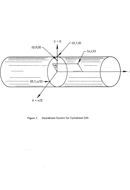
r'/a). The coordinate system is shown in Figure 1. The point source of

current located at

(O,R,O)·,

where R

<

1, is represented by the three-dimensional

delta function in (2ol), and is turned on abruptly at t

=

0,

represented by

the unit step function u(t) in (2.1). As shown in Reference 1, if the units of

u(t) are amperes, then the scaling for Vis V

=

aOiV'

1

where V' is the

paten-tial in volts.

The first equality in the boundary condition (2.2) expresses continuity

of the normal component of the current density crossing the membrane (more

2

-

+

precisely, a

times the current density).

The superscripts

and

represent

the conditions just inside (r

=

1-), and just outside (r

=

1+) the membrane,

respectively.

The ratio of interior to exterior conductivity is denoted by

a

=

oi/0

0•

The second equality in (2.2) relates the current crossing the

membrane to the electrical properties of the membrane, which is assumed to

have a capacitance C per unit area in addition to the conductivity o •

The

m

m

time variable is dimensionless and is related to the real time t'

by

t

=(a

/C o)t

1

•

For a derivation of (2.1) and (2.2) the reader is referred

m m

. 1

8=0

(0,1 ,0)

(x,r,8)

X

8

=1r/2

[image:12.627.104.541.89.730.2]

The boundary condition (2.3) assumes the zero reference for the potential

is at infinity. The initial condition (2.4) requires a finite time for the

membrane capacitance to accumulate charge, that is, (2.4) implies that a charge

+

-and hence a potential difference V - V cannot appear across the capacitance

instantaneously since an infinite current density at t = 0, would be required.

Such infinite currents are not possible because of the finite conductivities

of the interior and exterior media.

Observing that V(x,r,8,t) must be an even function of x, we can solve for

the potential by first taking the Fourier cosine-transform in x of Equation

(2.1).

Defining the Fourier cosine transform by

00

¢(k,r,8,t)

=f

coskx V(x,r,8,t) dx (2.5)

- 0 0

the Fourier transform of

(2.1)

is

1

- o(r-R)o(e)

r

(2.6)

=J

2

1T -in8

W

(k,r,t) e ¢(k,r,8,t) d8

n (2.7)

0

equation

(2.6)

may be transformed to

!

_l (

~)

- (

k

2

+

n

2

) '''

= -

!

6

(r-R)

( )

r

dr

ar 2 ~n r u t

r

(2.8)

This is a doubly transformed representation of our original Poisson equation.

Using the transforms (2.5) and (2.7) on the boundary conditions (2.2) and (2.3)

and on the initial condition (2.4) for V(x,r,8,t), the corresponding conditions

on

tJ;

(k, r, t) are n

1 atj;n

-

₁ dt/J + _n atJ;+ - atJ;t/J+

-= - - - -=

_t/J~

+ __ n_- n

_(2.9)

lJ;

(k,r,t)

n 0 at r

=

00

,,,- at t 't'n

(2.10)

(2 .11) Integrating

(2.8)

across the delta function, from r

=

R to r R+, shows that there is a discontinuity in the derivative of

lJ;

given by

n

+

3l]; (k,R ,t)

n

3r

31J; (k,R-,t)

n

3r

u (t)

- - R - (2.12)

The inhomogeneous equation

(2.8)

may be replaced by the corresponding homo~-eneous equation plus the jump condition (2.12) on the r-derivative at r

=

R.

In each of the three.regions

0

< r < R,

R

< r <

1

and

1

< r < oo, the right hand side of

(2.8)

is zero. The solution to this homogeneous equation in each

region is a linear combination of the modified Bessel functions I (kr) and n

K (kr). The solution which is finite at r

=

0

and which satisfies the boundary

n

condition (2.10) at r

=

oo is of the form

lJ;

(k,r,t)

n

a (t) I (kr)

n n

b (t)I (kr) + c (t)K (kr)

n n · n n

d (t) K (kr)

n n

O<r<R

R<r<l

l<r<oo

If the first derivative has the finite discontinuity (2.12) at r

itself must be continuous. Thus, from (2.13),

c (t) K (kR)

n n

Substituting the form (2.13) in the jump condition (2.12), we obtain

[ b ( t ) - a (t)l I'(k.R) +c _{n n ~ n n} (t) K'(k.R) _n = - uk.R(t)

and substituting (2.13) in the r

=

1 boundary condition (2.9), we obtain the two equations

(2.13)

R,

lJ; n

(2.14)

~

_E

[b (t)I'(k)

_n

_n

+

c

_n

(t)K'(k)J

_n

=

___!:

d (t) K' (k)

sa n

n

= (d

+d )

K (k) -

(c

+C )

K (k) - (b

+b )

I (k)

n n

n

n

n

n

n n

n

(2.16)

where a dot denotes differentiation with respect to time.

Equations (2.14) -

(2.16) are four equations which may be solved to obtain

the functional form of a

(t),

b

(t),

c

(t)

and d

(t).

If we solve (2.14) for

n n n n

a

_n

- b

_n'

substitute the result in (2.15) and solve for en' using the Wronskian

we obtain

I (kR) K' (kR) - K (kR) I' (kR) ==

n n n n

c (t)

n u (t) I (kR) n

and consequently

a

_n

(t)

_·

=

b (t) - u(t) K (kR)

_n

_n

l - k.R'

Substituting the result (2.17) for c

in the first of Equations (2.16) we

n

obtain an expression for d

in terms of b ,

n n

+

au(t) I (kR)

n

(2.17)

(2.18)

(2.19)

Substituting (2.17, (2.18) and (2.19) in (2.13), we obtain an expression

for the double transform of the potential in terms of only a single

unkno~

function b (t).

n

\jJ (k, r, t)

n =

b (t) n

Ct.b ( t)

n

I (kR) n

I' (k) n K' (k)

n

r

(kr) K (kR),

O<r<R

+

u(t)

n

n

I (kR) K (lcr),

R<r<l

n

n

(2.20)

K (kr)

+

Ct.u(t)

I (kR)

K (kr), 1<r<oo.

In order to obtain the potential V(x,r,8,t) we now need to determine the

func-tional form of b (t) and then take the inverse transforms

n

00

in8

1

L

tj;

(k, r, t)

¢(k,r,8,t)

₌

_2;r

_n

e

n=-00

and

00

v

(x' r'

e'

t)

~t[

coskx ¢(k,r,8,t) dk

of (2.20).

Using (2.17) and (2.19) in the second of Equations (2.16) leads, after

(2.21)

(2.22)

some algebraic man"ipulation, to the following differential equation for b •

_n

b (t)

+

n

[

~I'

_{E n}

(k)K' (k)

_n

]

I (k)K'(k)- ai'(k)K (k)

+

l bn(t)

n

n

n

n

I (k.R)K' (k)

n n

I (k)K

1

_{(k)- ai}

1

_{(k)K (k)}

n

n

n

n

Equation (2.23) is of the form

b (t)

+

p b (t) = q u(t)

+

s o(t)

n n

for which the solution is

[!(a-l)K

0

(k) -

~ K~(k)}u(t)

+

(a-l)K

0

(k)O(t)]

(2.23)

(2.24)

(2.25)

Using the appropriate form of p,q, and s which appear in (2.23), in the solution

(2.25), we find after more algebraic manipulation and use of the Wronskian of

I

and K ,

b (t)

n

u ( t) I (kR) K T (k)

n n

ki'(k)K' (k)

+

EI (k)K'(k)- Eai'(k)K (k)

n

n

n

n

n

n

K' (k)

{

ki'(k)K'(k)

n n

• E ( a-1) Kn (k)-kK

~

(k)o - _n --I--....,...(k-:)-K--:.-'-:(-k..,-) ---a-I..,...'

...,.(k"""'),__K_(,__k~)

- - - - 1

n

n

n

n

Noting that

3

'

4

(X)

-

1

-

1

dk coskx

~

27T2 0

_{n=_ro}

L.J

in8

e

l

I

(kr)

K (kR) ,

n n

I (kR)K

(kr),

n n

1 (

2

2

2

)-1/2

=

₄

7T ~

+

r

+

R - 2rR cos8

,

(2.26)

O<r<R

R<r<l

(2.27)

we can take the inverse transforms (2.21) and (2.22) of (2.20), with b (t)

n

given by (2.26).

Inside the cell, for 0 < r < 1, t

>

0, the potential is

V(x,r,8,t)

=

4

; (

x

2

₊

_r

2

₊

_R

2

_{- 2rR cose)-l/}

2

(X)

l

oo

f

I (kr) I

(k.R)

K' (k)

+

--2

~

ein8

dk coskx

n

n

n

---

ki

1

K'

+

EI K

1 -

Eai'K

27T

n=-oo

0

n n

n n

n n

• [E(a-l)K

_n

-kK' -

_n

(

ki'K'

)

l

K'

-

I

K'~~

1

K

+

E

·%

n n n n n

I K

1

_-ai'K

_e

n n n n

(2.28)

where for brevity we have deleted the argument of I

and K whenever

it

is k.

For the outside region, 1

<

r

< 00 ,

t

>

0, we substitute (2.26)

and do the following manipulations for the time independent part of

I I

n

abn(oo) K' Kn(kr) + ain(kR) Kn(kr)

n

I

I'[E(a-l)K -kK']

ai

(kR) K (k ) n n n

+

1

n n

r

ki'K'+EI K'-Eai'K

n

n

n

n

n

n

-EK I' + EI K'

( ) n

n

n n

ain

kR

Kn(kr)• ki

1

_{K'+EI K'-Eai'K}

n n

n n

n

n

- Eak I (kR)K (kr)

n n

ki'K'+EI K'-Eai'K

n n

n n

n n

in (2.20),

\jJ :

n

The inverse transforms (2.21) and (2.22) of (2.20), with b (t) given by (2.26)

n

yields, for the outside region, 1

<

r

<

oo, t

> 0,

v

(x, r'

e'

t)

a2

_~

~

_e

in8

fro

_{dk coskx ki}

1

Kn (kr) In (kR)

_{K'+EI K}

1

_-Eai

1

_K

2TI

Il=_oo

0

n n

n n

n n

I'K'

E n n

-

k-I K'-ai'K

n n

n n

n n

~

kl

'K'

(2.29)

Equations (2.28) and (2.29) express the general solution for the potential

inside and outside the cylindrical cell, respectively, for a point source of

current inside the cell.

In most of the remainder of this report, we will

III. STEADY STATE:

ASYMPTOTIC EXPANSION FOR HIGH MEMBRANE RESISTANCE

In this section, we investigate the steady state behavior of the

potential for small

E.

Letting t

=

00

in the formulas

(2.28)

and

(2.29)

for

the inside and outside potentials, respectively, we obtain for

0 <

r

< 1,

V(x,r,8)

4TI l ( 2 X

+

r 2

+

R 2 - 2rR

cose

)-1/2

00

+

_1_

~

e in8

j

0

dk coskx In (kr) I (kR)

2n 2

n~

n

_kl' (k)K' (k)

+

El (k)K' (k) - Eai' (k)K (k) [ £(a:-l)K (k) - kK_{n n} 1 {k)] K' (k) _n

(3.1)

n

n

n

n

n

n

and for 1

<

r

< oo

CXl

V(x,r,8)

co

f

K (kr)I kR)

- Ea2

~

e in8

dk cosk.x •

l •

n

n

~

k ki'K'+ci K'-cai'K

27T

n=-00

0

n n

n n

n n

(3.2)

where we have defined the steady state potential by V(x,r,8)

V(x,r,8,oo).

A.

Potential Inside the Cell

First, we will consider the inside potential, (3.1).

It consists of an

algebraic term which is just the free-space potential of a unit point source

at (O,R,O), and a complicated term which is an infinite sum of integrals

(Fourier transforms).

We would like now to study the small £behavior of

(3.1) by expanding the integrals in powers of

£,

and interchanging the order

of integration and summation over powers of

£.

This results in an asymptotic

representation of (3.1) in the

£ ~

0 limit. The procedure is straightforward

We start by expanding the fraction appearing in the integrand

in

(3.1)

in powers of E, treating E as a small quantity.

We find

E(a-1)

K

1 -

n

[E(a-l)Kn - kK'JK'

K'

k

. ·K'

n

n

n

n

ki'K'

+

EI K' - Eai'K

-yr

K

n n n n

n n

n

1

₊

~n

_I~

n

-

CXl('

n

r

I)

K'

E

n

n

n

k

K'

- I '

- y

₁

₊

n

n

n

f

K)

E

n

n

l

+

k

I~-

a

K~

K'

[1

1

- a

~~)

l

n

!;:

I'"

+

k

2

I'K'

c

n

1

E

n

n n

+

k

I~

K'

·r+

• { 1 -

~ (~!

-

a

~)

+ ..

~}]

n

E

(3.3)

- I '

k

2

I'

K'

n

n n

The third equality in (3.3) follows using the Wronskian of I (k) and K (k).

n

n

For sufficiently small E, and

a~l,

the expansion (3.3) converges for

k

I

0.

If k

+

0 and n

~

0, we have for the expansion of the function in the

integrand in (3.1) whose inverse Fourier cosine transform we must calculate,

-I (kr)I (kR)

n

n

K' [

{

(I

K )

ll

n E E n n

IT .

1

+

2 1 - k

I ' -

a

K'

+ .•

·JJ

n k I'K' n n

n n

-1

which converges absolutely if E

<

(1

+

a/n)

, so that the expansion (3.3)

may be used even when k

=

0

if n

~ 0.

On the other hand, if k

+ 0

and n

= 0,

we have

K' [

(1-

f(~h-a

:b)+ ... ]]

-I

₀

(kr)I

_{0 (kR)}

Ih

1

+

E

k

2

I'K'

0 0

2

[1-

2E

{1

~~

+ ... }]

(3.4b)

-

k+O

_k2

_k2

which diverges at k

=

0.

The expansion (3.3) thus may not be used when n

=

0.

We can, however, get around this difficulty by determining an explicit

expression for the remainder, for any finite number of terms in (3.3). We

will now do this for the first two terms in the expansion (3.3).

We begin

by separating the fraction in the integrand of (3.1) into its E

+

0

limit and

the remainder:

[ E (a-l)Kn -

kK~

J

K~

ki'K' + EI K'

Eai'K

n n

n n

n n

K' K'

c: - _E.

+

_E.

I' I'

n n

[

E(a-l)K I' - kK'I'

_{n n}

_{n n}

J

• l

+

-k-I-=,-K-=,-+-E_I_K...,,,---_-E_a_I--:-

1

K-n K-n

n n

n n

K'

K'

-E(K I' - I K')

n

n

n n

n n

- V

+

V •

ki'K' + EI K' - Eai'K

n

n

nn

nn

nn

K' K'

n E n 1

-v-k rr

ki

1

K

1

+ EI K

1 -

Eai'K

n n

n n

n n

n n

(3.5)

We can continue this process, and now isolate the

0

(E) term as well. To do

this, we write

1 1 1

+

ki'K' + EI K' - Eai'K

ki'K'

ki'K'

n n

n n

n

n n n n n

1 1

ki '

K'

+

-k-I-=-'

K='

-n -n n n

ki'K'

n n

-[kl'K'

n n

+

EI K'

_{n n}

Eai'K

ai'K - I K'

n n n n

n n

ki'K' + EI K' - Eai'K

n n n n n n

and substitute in (3.5) to obtain an 0(1) term, an 0(£) term, and the

remainder:

[s(o.-l)Kn -kK'JK'

_n

_n

K'

_n

_s

_£ 2 ₁

(3. 6)

kl'K'

₊

t:I

K' - so.I'K

-I'-

_k21",2

k2I,2

ki'K'

n n n n n

n

n

n n

n

n

ai'K

- I

K'

- E

n n n n

Note that the first two terms in

(3.6)

are identical to the first two terms

in

(3.3).

We could obviously continue this process indefinitely and thus obtain an

asymptotic expansion for

V

to any desired order in

£,

but we

will

stop at

this point and be content with an expansion correct to

O(c).

Substituting

(3.6)

in

(3.1)

we obtain an expression for the potential

inside the cylinder,

1 2 2 2 -1/2

V(x,r,8)

=

4TI

(x

+

r

+

R -

2rR cos6)

1

~

in6

/oo

- -

₂

LJ

e

dk coskx In (kr) In

(kR) 21T n=-o:> ₀

1

ki'K'

n n ai'K - I K'

n n

n n

(3.7)

It is not permissible to discard the last term in the square bracket in

2

(3.7},

which at first glance appears to be of

O(t. ),

because when n

==

0

its

contribution to the integral is of lower order.

We

kne~ in

advance, from the

divergence of

(3.3) at n

=

0, k

=

0, that this must occur since the first two

terms

[0(1)

and

O(t.)]

in this case do not correctly represent the integrand

in (3.1).

I ' (k) K' (k) "' n n

I' (k)K (k) n n

I (k)K' (k) n n

I

- - k n -2 2

1

-2

if n ~ 0 if n

=

0

!

-

~

_!_ k - l k log k if n i f

~

0 n

!

-

-k~

.!_

1

k-l if n i f n = 0 ;.o 0 0

Consequently we have for the limiting behavior of the function whose inverse Fourier cosine transform is to be calculated in

(3.7),

for n ~

0,

k + 0,

ki'K'

1

l

--:---:-n n _ £

ai 'K - I K' n n n n

k+O

r'1ln • [ -

2~

+

4:2 -::2 •

n 1 +a

J

+

£(l+a)

The last term is 0(£2) for n

~

0, k + 0. Since ki'K' • (ai'K - I K')-l is n n n n n n

also nonzero for any k > 0, the third term is 0(£2) for all k and may be omitted in the 0(£) calculation of the potential.

The corresponding term for n

=

0, however, cannot be omitted. It is 1

kil

+

£Io IlKO

1 + a r K 0 1

IS_

(k) I

1 (k) k+O

1

l

+

Retaining terms up to and including

O(E),

the inside potential (3.7) becomes.

V(x,r,S)

=

4

;

(x

2

₊

r

2

+

R

2

- 2rR cos8)-l/Z

00

-

~

'2::

einBJ

00

dk

cosk.x In (kr)In (kR)

2TI n=-00 0

K'

2 0

n0

n

E E 1

0

(3.8)

rr+

_{k21,2 - k212}

kll

n

n 1

IlKO

+

sr

0

l+a

-L

ro~

V(x,r,8)

00 00

L

ein8

1

dk

n=-00 0

00

+~

f

dk

2TI

0

ro

(kr)

ro

(kR)

2

E (

2

2

kll

+

k2

+

k2 1r R

-_ -_ -_ I_K_

+

t:IO

l+a _!_0 1

_oS

(3. 9)

+ •..

and all integrands in (3.9) are well behaved at k

=

0.

The first two terms in (3.9), the inverse distance term and the infinite

sum, appeared in identical form in Equations (5.2) and (5.3) of our earlier

2

report for the a

=

0 case.

In that report it was demonstrated that for large

x, the sum of these two terms was exponentially small.

The rest of Equation

(5.3), which survives for fixed /Ex in the limit

E +

0, was called the

*

*

"far-field potential," and designated by W(x ,r), where x

IE

X (1- t:/8

+ ... )

00 U(x,r) =

~

j

dk

2n

::J

+) +)

(l-r

2

-R

2

- : 2

)1

+

£Io

J

(3 .lOa)

OJ

=~

f

dk

2n

o

_[

k2 2 2

2

l +

4

(r

+ R ) + .••

coskx -

4

E •

--~----,-(

---;:;-\2)-k4

~2 (11~2

+

a~2

[y

+

log

n)+£

1+

~

+

+3._+_£(1-

r

2

- R

2

-

-4-)l

k

2

k

2

k

(3.10b)

00

=

~

j

dk coskx

2n

o

[

{

2+R2

k)}

kz{l

k)}

]

1 +

E

t-

~-

a(y+log

₂

+

2

tta<y+lo~

+ •.•

( 2) 2 { k 2 k 2 ( k ) }

E

1+

~

+

~

1 +

8

+

a

2

y

+ log

2. +

(3.10c)

1

oo [ ( 2 2) £

2

[l-4a(y

+

log

k₂)]

2

+

E

1-r -R

+

dk coskx ₂

+

2

0 k

+

2E ( k2

+

2E)

..

·]

In (3.10b) we have replaced the modified Bessel functions by their expansions around k

=

0; y is Euler's constant; in (3.10c) we have combined the three terms over a single denominator, and the asymptotic result of (3.10d) follows since in the E + 0 limit the integral comes increasingly from the vicinity of

2

k = 0 and hence k may be treated as a small quantity.

That (3.10d) is the asymptotic representation of (3.10c) in the E + 0 limit can be seen most easily by making the change of variable k2

=

E s2, so that (3.10c) becomes

---1

ds cos

(z;;/E

x) 2 2 2 .

1 oo

[~

+

E{t -

r2 ;R2 -

a(Y

+

~log£

+

~og f)(~

-

~2)+ ~2}+

0

(£21

2n2/£

o

~

+

~

+ EZ { l +

t

+

"~2(r~ ~og

£ + log

~)

}+ o(£2)

Expanding the expression in square brackets in ascending orders of E and converting back to the original variable k, we obtain (3.10d).

As

k + 0, the denominator· in (3.10c) approaches E; i t is O(E) if

k <_

~

L 112

•

c

onsequent y, 1 th e 1n egran 1s . t d . 1 arge, 0( E -l) , 1 'f k < - E 112 • In the E + 0 limit, the integrand becomes increasingly large in the vicinity of k

=

0,

but this behavior is confined to an increasingly narrow range of k. As a result the major contribution to the integral itself, in the E + 0 limit, comes from a range of k between zero and a small value which is

O(s

1/2). Replacing the expression in square brackets in (3.10a) by its expansion around k

=

0 therefore leads to an asymptotic expansion for the integral. This is Laplace's method for obtaining an asymptotic representation of an

. 1 5

1ntegra • From this discussion, i t is clear that in making the expansion, 1/2

k and E are to be treated as small quantities of the same order of smallness.

2

·z

[

}

_ 2

+

E:

(1-r -R )

-x&

a&

-x/2£{(!_ _

v - l l o g

!:.)

(1

+

x/2c:)

+

1

U(x,r) - _ __..:...___:....---~ e

+

8n e 4a ' 2 2

4n/2E

'

-

~I

ex& (l-x&)Ei( -x/2£)- e-x& (

l-lx/2£)

Ei (

x/2£)

1]

6

To obtain

(3.11)

we have used

00

f

cos bk S2+k2 0

n -bS dk =

2S

e

7 to obtain the first term and

1

oo Sdk

n

-

b S

n [

b S . - b S .

J

log ak cos bk

=

2

e log aS

+

4

e E1(-bS)- e E1(bS)

0

82+k2

(3.11)

to find the second term, where Ei(~) is the exponential int~ral. Differenti-ating B-l times the last integral with respect to B, we obtain

dfoo

dk dB log ak cos bk

2 2

0

s

+k

so that

~ d~ ~

[-

~

e-bB log aB + ;;- {ebB Ei( -bB) - e-bB Ei(bB)}

J

- B;

[~e-bB

log aB +*{ebB Ei(-bB)- e-bB

Ei(bB)~

+

i [

~

(

-b log aB +

~)

e-bB +

~

b { ebB Ei (-bB) + e-bB Ei (bB) }

J

Letting

log a

= -

1

4

a

+

y - log 2

b

=

X

we obtain the last term in

(3.11).

Regrouping the terms in

(3.11)

according to their order in €, we have

(

x )

1

-x

U

liE ,

r

=

2n/2E e

I2E [

-x {

5 2 2

a

£ - (1

a.

€)}

+

Bn

e

4 -

r

-R -a.(y-1) -

₂

log

2

+

x

4 -

ay -

2

log

2

a

x

-

- -

a

-x

-

- . -

J

- 2

e

(1-x)

Ei(-x)

+

₂

e

(l+x)

E1(x)

+ ...

(3.12)

where we have defined a far field coordinate by

x

=

/2£

x. It may be seen that for large

x,

(i.e., if the product

x •

€ is not small) the expansion

(3.12)

is not asymptotic because the second term [0(£

1

/

2

)]

is not small com-pared to the first term [0(£-l/2)]. This nonuniformity for large

x

can be removed by making a change of variable to

x

x

(1

+

n(E)

+ ... )

X x (1- n(c)

+ ... )

(3.13)

where n will be chosen to make

(3.12)

uniform in X. Expanding the exponential integrals in a Taylor series around ± X, we have

Ei(±X)

=

Ei(±X(l-n+ ••• ))

=

Ei(±X) - ne±X

+

(3.14)

and doing the same for the exponentials in

(3.12),

we have

Substituting (3.14) and (3.15) in (3.12), retaining terms up to and

includ-ing 0(£

112

), and defining the far field potential Win terms of the far field

axial variable X we obtain

-1/2

r

U(E

X(l-n+ •.. ), r)

- W(X,r)

= 1

e-X(l+Xn)+

/2E

[e-X{~-

r

2

- R

2

-

a(y-1)-

~log.£

2n&

8n

4

2

2

+ X(! -

a-y -

~

log

.£) (

4 2 2

I

-

~

eX(l-X) Ei(-X)

2

a

-X

J

+

-z

e

(l+X) Ei(X)

(3.16)

.

-1/2

where we have used the first two terms of (3.15) in the

O(E )

term of

(3.12) but only require the leading term of (3.14) and (3.15) in the 0(£

1

/

2

)

term of (3.12).

In order to make the coefficient of X e-X vanish in (3.16),

we choose

and, substituting in (3.13), X is given by

X

~

12£

X [ 1 -

E(i -

~

-

%

log } )

+ •••

J

(3 .17)

and consequently W becomes

1

w

=

-2ni2E

-X

rzE [

-X{ 5 2 2

a

E }

e

+ ---

e

- - r -R

-a(y-1) - -

log

-81T 4 2 2

-%

eX(l-X) Ei(-X)

+

~

e-X(l+X) Ei(X)J

+ •••

(3.18)

*

of Reference 2, we see that

(3.17)

and

(3.18)

reduce to that formula when a =

0.

A

second, and perhaps more important reason for redefining the far field variable is that

/2£

x, the leading term in X, is a variable often used in the physiological literature. Thus

X

is the direct generalization of the common physiological variable to higher orders of E.

Using the asymptotic formula for the exponential integral

ex (

1

2!

3!

)

Ei(X)

"'-x

l

+ - + - + - + ...

x x2 x3

the combination of Ei (X) and Ei (-X) in

(3.18)

is, for large X:

(3

.19)

Thus, for sufficiently large X, the far field potential W will be domin-ated by the exponential integral expression in the O(E112) term, rather than by the leading O(E-l/2) term. This is not a nonuniformity in X, in the same sense that the form

(3.12)

is nonuniform in

x.

It merely means that the far field W is composed of two parts: an ordered sequence of exponential terms, and an ordered sequence of exponential integral terms. The former begin with

-1/2

.

1/2

O(E ), the latter w1th O(E ). If we continued the expansion

(3.18)

to higher order, we would expect the exponential integral terms to be of increas-ing order in E, uniformly in X. Thus, each of the two ordered sequences is uniform in X but one depends on X exponentially, the other as an exponential integral.

For X of 0(1), the far field decays exponentially. However, if

X -X

_{e < < E (3.20)}

a

In a typical physiological case, say E

~

10-3, a= 0.3, the two sides of (3.20) are equal for

X

~ 10. For

X

5

the left hand side is

100

times the right hand side. At this point the potential

(3.18)

has decreased to

7

x

10-

3

times its X = 0 maximum. Consequently, at any position where the exponential

integral is of significant magnitude relative to the exponential, the total

potential is so small as to be of no experimental significance, and we

con-elude that the exponential integral terms are of no practical importance in

the interior of the cell for typical experimental situations. We will see

below that the situation is somewhat different outside the cell, where there

is no 0(£-l/2) term, .and the exponential integral can be the dominant term.

In addition, in Section

V

we will discuss the sinusoidal steady state, in which case a complex "effective" E can be defined which is a function of

frequency, and whose magnitude can be much greater than 10-3• In this case

the exponential integral can be important inside the cell.

Using the definition

(3.16)

of Wand (3.10) of U, we can substitute the expression

(3.18)

for Win (3.9) to obtain an asymptotic representstion of the potential which is valid for all x. It is

V(x,r,6) 1 _e

-X

₊

1

2 2 2 1/2

4TI (x

+

r

+

R - 2rR

cos8)--

2

~2

too

einS

~oo

dk coskx [

;f

In (kr)In (kR)

+

2

:~

J

a/2'€

log

£

-X

16n

e

I2E [

-X { 5 2 2

a

}

a

X

+

₈

7T

e

4-

r - R -

a(y-1)

+

₂

log 2 -

₂

e (1-X) Ei(-X)

with X related to x by (3.17). In (3.21) we have arranged the terms in

. . -1/2 1/2 1/2

ascend1ng order of£ [v1z., 0(£ ), 0(1), 0(£ log£), 0(£ ), O(E)~ ••• ].

This is the generalization to arbitrary

a

of Equation (5.3) of Reference 2. It is noteworthy that the leading, 0(£-l/2), term, as well as each term whose order is an integer power of £, are independent of

a.

There is no effect of the external medium conductivity until the third term in the expansion.

The two terms in (3.21) which are infinite sums of inverse Fourier trans-forms are identical to the corresponding terms in Equation (5.3) of Reference 2. The sum in the 0(1) terms can be computed most efficiently for x > 0.5 by converting the integral to the sum given in Equation (4.31) of Reference 2, or, for x < 0.5, to the more complicated sums given in Equation (D.l4) of Reference 2. The sum in the 0(£) term can be computed, for any x, by converting the integrals into the sums given in Equation (C.9) of Reference 2.

We would now like to obtain an asymptotic representation of the inside potential which is useful in the "near field." More precisely, \ole seek an expansion arranged in ascending orders of E when x is held fixed as £ ~ 0 [rather than holding X fixed as E ~ 0, as was done in (3.18)]. Using (3.17) to express X, the far field variable, in terms of x, the near field variable, the Taylor expansion of the exponential yields

-X

e

and the Taylor expansion of the exponential integral yields e-X(l+X) Ei(X) - eX (1-X) Ei(-X)

=

2/2E x + 0(£3/2 log £).

3

~

+ 0(£2 log E)

6

V (x, r, 6) 1

X 1

2

2

2

8)-1/2

- - + -

(x

+

r

+

R - 2rR cos

2Tr

4Tr

co <Xl

l

K' 200n

J

1

2L

e

in8

~

dk coskx •

I: In(kr)In(kR)

+

-1.:2

2Tr

n=-oo

a& log

E

16Tr

/2E

u-

2

₂

₂

₁

₁

+ - -

_8Tr

T -

R

+

2x -a(y-1-

2

log 2)

00

Ex (

2

2

2

2)

£

L

inS

-

_4Tr

_{1 - r - R}

₊

3

X -

27T2

e

n=-oo

coskx

d k •

----::--k2

_[

I (kr)I

(kR) (

• _ n -::--n

+

_{1 _}

I'2

n

+

2

r - _R2_-

_{!!_ )}

_o

J

k2

On

(3.22)

Equation (3.22) is the generalization of Equation

(5.2)

of Reference 2 to

arbitrary

a. As in that case, it is not uniform in x, but fails to be

asymptotic for large x.

B.

Potential Outside the Cell

We now return to Equation (3.2) for the outside potential and proceed to

obtain an asymptotic expansion in powers of

£,

using the same approach as was

just applied to Equation (3.1).

Separating the integrand into its

£ ~

0 limit

plus the remainder [see the equation preceding (3.6)], we obtain from (3.2),

for the potential in the region 1

<

r

< oo,

V(x,r,S)

£0:

- 2Tr 2

<Xl

n=-oo

00

ein8j

0 • [

1

+

ki'~'

_{n n}

_£

l

a:I'K I K'

As we have found above when considering the corresponding terms in

(3.6) -

(3.8), the second term in the square brackets in the (3.23) integrand

is 0(£) unless n

=

0, k

2

<

£ , in which case it is 0(1) and must be included

in our calculation of

v.

For n

0, the integrand in (3.23) is

cos kx

K

0

(kr)r

0

(kR)

rl -

E ]

k2

1

1

(k)Kl (k)

ki

1

K

1

+ £

o.11KO+IOK1

coskx

K

0

(kr)r

0

(kR)

[ 1

-£10

k2

1

₁

(k)K

₁

(k)

£10 +

kil

]

11KO

1

+a

ro~

(3.24)

where we have expanded the Bessel functions around k

=

0 and deleted terms

2

of higher order than O(E) or O(k ) to obtain the last term in the square

brackets.

Note that since there is an overall factor of £ multiplying (3.2),

we need to retain one less order of £ or

k

2

than we did for the corresponding

step for dealing with the potential inside the cell.

Substituting (3.24) in

(3.23), we obtain

CXl

_ ca

2

'

in8/

00

dk

V(x,r,e)

= ~

e

-z

coskx

21T n=...co 0 k

Kn(kr)1n(kR)

2c(y

+log

~)onO

]

K'

(k)1' (k)

-

k 2

+ ••.

n n

₂

+

E:

(3.25)

Once again, we wish to separate this integral into two parts but

V (x, r, 8) =

e:::a

2 7T

~

ein8

/oo

dk

[Kn (kr)In

(k.R)

6

2

coskx

I'(k)K'(k)

n==-oo

0 k n n

(X)

dk coskx

kr

y +log

2

2

k

+

2E:

+ ...

- 2(y +log kr) 0

₂

_nO

J

(3.26)

With this separation, the first term is clearly O(e:::) since all E-dependence

has been removed from the integrand.

The second term, however, is O(e:::

112

) as

will be

sho~~

below.

The term log (kr/2), which originates from the expansion

of K

0

(kr) in (3.24) restricts the validity of our asymptotic expansion to

values of r which are not too large.

In order for the first term of the

expansion to approximate K

0

(kr) adequately, the product kr/2 must be small.

Since the last integral in (3.26) originates mostly from the range

0 < k <

E

112

(the integrand being negligible fork> > E:

112

), if r satisfies the condition

1

2

r

< <

E:-l/2,

kr/2 will be small for values of k contributing significantly to the integrand.

Our asymptotic expansion will only be valid for this restricted range of r,

which is adequate for essentially all experimental situations. Letting

log a

2E:

r

-y

+

log

₂

s2

in the tabulated integral

7

used to obtain (3.11), the last integral in (3.26)

can be evaluated:

kr

00

_{y + log}

2

f

dk coskx •

Q k2

+

2E:

= _7T_

[ze-/7£ x (y +log

/".f"

r)

4&

&

+

e

X

Ei

(-/2E

X)-

e

-/2s

X

Ei

(rzE

x)]

the outside potential the asymptotic representation uniform in x, for the d . 1 . bl . h 1 - l / 2

ra 1a var1a e 1n t e range ~ r << £ ,

[

K (kr)I (kR)

J

coskx

I~(k)K'~k)

- 2(y +

logk~

) onO n n

n=-oo

+ ...

(3. 28)

-1/2

Because of the absence from

(3.28)

of a term of 0(£ ), as was present in

(3.18)

for the inside potential, the exponential integral is relatively more important in the expansion of the outside potential. In the first line of (3.28), the exponential integral terms dominate the exponential for values

-3

of X greater than about 1.5 if E ~ 10 . It should be remembered that since

-lj2

the O(E ) and 0(1) terms are missing from (3.28), the outside potential is much smaller than the inside potential. Compared to the inside potential, the exponential integral terms would again be less important.

Substituting

12£

x for X in (3.28) and expanding in the limit E ~ 0, we have

-X ~

e

=

1 -

v2E x

+ ...

eX Ei(-X) - e-X Ei(X) 2X log X-

2(1-

y) X+ •••

=

12£

x log £ +

212£

x (log x +

~

log 2 + 1 - y) + ••• which, when substituted in (3.28) leads to the near field expansion of ·the

V (x, r, 6)

-

~

lfS

log £

81T

- __£__

&(r

+

~

log

~)

4TI 2 2

O.XE (

-2iT

1

-co

2x)

O.£ ' " "

2y+log

r-

--2

L;

2TI n=...oo

co

ein6

f

dk coskx

7

0

[

K (kr)I (kR)

J

•

-I-=-~-=-(

k--:-) K-,':-C-:-k-=-)- - 2 ( y

+

10 g

~r

) 0 n 0 n n

IV. RELATION OF THE STEADY STATE EXPANSION TO A SINGULAR PERTURBATION ANALYSIS A. Far Field Potential

It is interesting to see how the present problem might be approached using singular perturbation theory. The problem specified by (2.1) - (2.4) can be decomposed into a sequence of problems each with physical meaning, cor-responding to a single term in the expansion of the potential in orders of E. It will then be seen that each term in the expansion obtained in Section III is the solution to one of these physical problems.

We consider the far field limit first. The singular perturbation analysis begins by expanding the far field potential in orders of E, the particular orders of E being chosen here because they appear in the exact solution. In an~ priori analysis using singular perturbation techniques, it would be necessary to show that this is the appropriate expansion and to consider the physical origin of the log E terms. Using the knowledge we have already gained from the exact solution, however, we can write the expansion:

W(X,r)

+

~3/2 3/2

e- logEW

312(X,r)

+

E W2(X,r)

+

(4 .1) The terms with integer subscripts correspond to the notation introduced in Reference 2 for the far field potential. The intermediate terms containing a log E were not present in the a

=

0 case of Reference 2 and we use the half-odd integer subscript to indicate between which two integer terms the term falls. The far field coordinate X is related to the coordinate x by the transformation

X

=

n(E)x

The Equation (2.1) and the boundary condition (2.2) can then be broken

down into the sequence of equations and boundary conditions

,_/ w

= 0

t

0

aw~

₁

aw~

dr ==

a

---a;-

= 0

aw~

₁₂

₁

awl/2

+

a

ar

--ar

2

a

2

w

0

v

_wl

2

-t

_ax

2

0

(4. 3)

(4 .4)

(4.5)

(4. 6)

(4. 7)

where

V

2

denotes the transverse Laplacian and

n(£) in

(4.2)

has been taken

t

equal to