A Logarithmic Finite Difference Method for Troesch’s Problem

ISSN Print: 2152-7385

DOI: 10.4236/am.2018.95039 May 30, 2018 550 Applied Mathematics

A Logarithmic Finite Difference Method for

Troesch’s Problem

M. S. Ismail, K. S. Al-Basyoni

Department of Mathematics, College of Science, King Abdulaziz University, Jeddah, KSA

Abstract

The aim of this paper is to derive a numerical scheme for Troesch’s problem and to overcome the difficulty which faces the existing numerical methods when considering the Troesch’s problem with large values of λ. A logarithmic finite difference method is derived for solving the Troesch’s problem. The method is very simple and works well for arbitrarily large values of the Troesch’s parameter. To test the proposed method, we have used a wide range of the Troesch’s parameter λ. A comparison with some existing methods is given. The numerical results show the robustness and the superiority of the proposed scheme over most of the existing numerical methods for the Troesch’s problem.

Keywords

Troesch’s Problem, Logarithmic Finite Difference Method, Inverse Sine Hyperbolic

1. Introduction

Troesch’s problem arises in the investigation of the confinement of plasma col-umn by radiation pressure and is defined by

( )

sinh

u′′ =

λ

λ

u ₍₁₎

subject to the boundary conditions

( )

0 0 and

( )

1 1

u = u =

₍₂₎

The main difficulty associated with Troesch’s problem is the boundary layer near x=1_{. Accordingly, many researchers try to solve this equation numerically,} some of these methods are: Sinc-Collocation method [1], the modified homoto-py perturbation technique [2], a smart nonstandard finite difference for second order nonlinear boundary value problem [3], the finite element method and How to cite this paper: Ismail, M.S. and

Al-Basyoni, K.S. (2018) A Logarithmic Finite Difference Method for Troesch’s Problem. Applied Mathematics, 9, 550-559. https://doi.org/10.4236/am.2018.95039

Received: March 26, 2018 Accepted: May 27, 2018 Published: May 30, 2018

Copyright © 2018 by authors and Scientific Research Publishing Inc. This work is licensed under the Creative Commons Attribution International License (CC BY 4.0).

http://creativecommons.org/licenses/by/4.0/

DOI: 10.4236/am.2018.95039 551 Applied Mathematics discontinuous Galerkin methods [4] [5], and the shifted Jacobi-Gauss colloca-tion method [6]. A cubic spline collocation method is given in [7]. All of these methods provide a numerical solution of Troesch’s problem for moderate values of λ. Recently, an accurate asymptotic approximation of Troesch’s problem with large values up to λ =60 is reported in [8]. For more details see [9] [10].

This paper is devoted to derive a logarithmic finite difference method as a new method to solve the Troesch’s problem for arbitrarily large parameter λ.

The paper remaining of this paper is organized as follows. In Section 2, we de-rive the numerical scheme as well as a fourth order finite difference scheme. Sec-tion 3 is devoted for the numerical results and comparisons with some existing methods. Concluding remarks are given in Section 4.

2. Numerical Method

In order to derive the numerical method for solving Troesch’s, we present the following definition.

Definition: The inverse sine hyperbolic function is defined by

(

)

1 2

sinh− x₌ln x₊ x ₊1 ,x_∈

(3) and its derivative is defined by

(

1

)

2

d _sinh 1 _.

dx x _{1 x}

− ₌

+ (4)

By using the previous definition, the Troesch’s problem (1) can be written as

(

)

(

(

)

2

)

1

1_sinh 1_{ln 1 ,}

u λu λu λu

λ λ

− _{′′ ′′ ′′}

= = + +

(5) which is the main point in this paper.

Using uniform mesh including

(

n+1

)

points 0=x0< <x x1 2<<xn=1, such that x ih ii= , =0,1, , n, where h=1 ,_n α−1=λh2. We denote the exact and the numerical solutions respectively by u x

( )

i and Ui at the grid point xi. Now by using the second order central finite difference approximation for the second derivative

( )

2

(

1 1

)

1 ₂

i i i i

u x U U U

h + −

′′ _ − +

(6) into the Equation (5), this will lead us to the logarithmic finite difference method

(

)

(

)

2

1 1 1 1

ln 2 2 1 0,

1,2, , 1

i i i i i i i

U U U U U U U

i n

α + − α + − λ

 _{− + +  − +  +} _{− =}

 

 

 

= _ −

(7)

subject to the boundary conditions

0 0 and n 1.

U = U =

₍₈₎

DOI: 10.4236/am.2018.95039 552 Applied Mathematics unknown solution

{ }

11

n i i

U ₌ . The details of the logarithmic can be given displayed by the following algorithm.

Algorithm 1. Logarithmic method

1) For i=1 _{using (7) and the boundary condition} U₀=0_{, we obtain}

(

)

(

)

2

2 1 2 1

ln_α U −2U + α U −2Ui  + −1_ λU =0

(9) 2) For i=2,3, ,_ n−2 _{we use}

(

)

(

)

2

1 1 1 1

ln 2 2 1 0,

2, , 2

i i i i i i i

U U U U U U U

i n

α _{+ −} α _{+ −} λ

 _{− + +  − +  +} _{− =}       =  − (10)

3) For i n= −1 _{using (7) and the boundary condition} Un=1 to obtain

(

)

(

)

2

1 2 1 2 1

lnα 1 2− Un− +Un− + α 1 2− Un− +Un−  + −1 λUn− =0

  (11)

Newton’s method is used to solve the nonlinear system which can be de-scribed in the following way.

Algorithm 2. Newton’s method 1) For s=0,1,2,_.

2) Solve the tridiagonal linear system ( )

( )

s

JZ F U=

for the unknown vector Z using Crout’s method. The elements of the function

( )

i i

F U and the Jacobian matrix J are defined as follows

( )

(

)

(

)

2

1 1 1 1

ln 2 2 1 0,

1, , 1

i i i i i i i i i

F U U U U U U U U

i n

α + − α + − λ

 _{ } 

= _ − + + _ − + _ + _− =

 

= _ −

(12)

and the Jacobian matrix has the tridiagonal structure

1 1

2 2 2

2 2 2

1 1

i i i

n n n

n n

b c a b c

J

a b c

a b c

a b − − − − −         =            

with elements defined by

(

)

2

1 1

, 2,3, , 1

2 1

i

i i i

a i n

U U U

α

α _{+ −}

= = −

 − +  +

 



(

)

2

1 1

2 _{, 1,2,3, , 1}

2 1

i

i i i

b i n

U U U

α λ

α + −

= − − = −

 − +  +

 



(

)

2

1 1

, 1,2,3, , 2

2 1

i

i i i

c i n

U U U

α

α _{+ −}

= = −

 − +  +

 

DOI: 10.4236/am.2018.95039 553 Applied Mathematics 3) Update your solution by using

( )s+1 ₌ ( )s ₋

U U Z

4) Repeat steps (1)-(3) till the following condition ( )s+1 ( )s

∞

− ≤

U U 

is satisfied. The constant  is assumed to be small.

The initial guess vector is taken as the linear interpolation between the given boundary conditions, and has the following form

( )0 _{, 1,2, , 1}

i i

U = =x ih i=  n−

The previous method is of second order accuracy and it works for wide range values of λ.

A fourth order finite difference method can be used for solving the Troche’s method for limited values of λ. This method can be given as follows.

By using the forth order approximation of the second derivative

( )

2

2 ,

1 1

12

i i

u x δ U

δ ′′ +  (13)

where 2

1 2 1

i i i i

U U U U

δ

= − − + +

Using this approximation and after some manipulation we will end with the following scheme

(

)

(

)

(

)

1 2 1 sinh 1 10sinh sinh 1 ,

i i i i i i

U₋ − U U+ ₊ =ω_ λU₋ + λU + λU₊ _

(14)

2

1 for 1,2, , 1, where ,

12

i=  n− w= λh

(15)

0 0 and n 1

U = U =

₍₁₆₎

The resulting method (14) is of fourth order accuracy. The numerical solution

{ }

1

1

n i i

U −

= in this case can be also obtained by solving the nonlinear tridiagonal system. Newton’s method is used to solve this system as we did before.

3. Numerical Results

To test the efficiency of the proposed method, we choose h=0.0005 and

12

10−

=

 , for the moderate values of λ=0.5,1,5,10_{. Comparison with some}

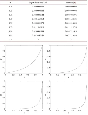
ex-isting methods is given in Tables 1-5. In Figure 1 we display the numerical so-lution for λ=3,5,8,10_{. The numerical results indicate that the proposed}

me-thod is highly accurate comparing to the published works.

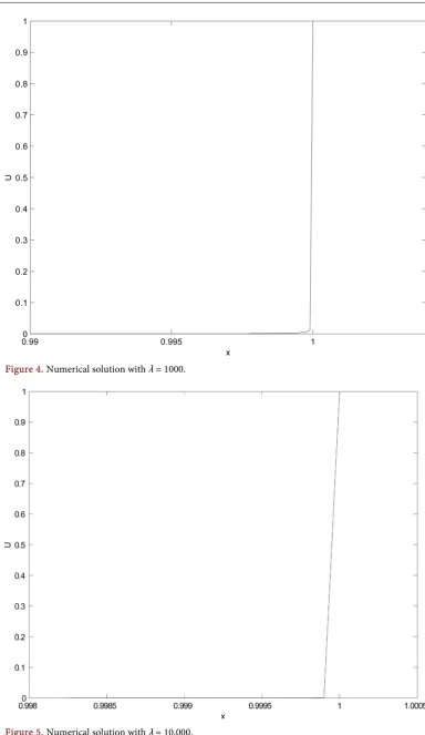
For large values of λ, we choose h=0.0001_{. In Table 6 and Table 7, we}

DOI: 10.4236/am.2018.95039 554 Applied Mathematics

= 100,200,1000,10000

λ _{in Figures 2-5.}

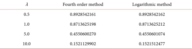
[image:5.595.207.540.177.376.2]

Finally, we tested the fourth order method and make some comparison with the logarithmic method, we have noticed that, the results produced by this me-thod are quite good for the small values of λ only, see Table 9, and the method is handicapped and fail for larger values of λ.

Table 1. Troesch’s problem with λ = 0.5 and h = 0.0005.

x Logarithmic method FDM [3] Homotopy [2] Doha [6] Exact

0.1 0.0959443493 0.0959443492 0.0959395656 0.0959443493 0.0959443493

0.2 0.1921287477 0.1921287476 0.1921193244 0.1921287477 0.1921287477

0.3 0.2887944010 0.2887944007 0.2887806940 0.2887944009 0.2887944009

0.4 0.3861848465 0.3861848462 0.3861675428 0.3861848464 0.3861848464

0.5 0.4845471649 0.4845471645 0.4845274183 0.4845471647 0.4845471647

0.6 0.5841332486 0.5841332482 0.5841127822 0.5841332484 0.5841332484

0.7 0.6852011485 0.6852011481 0.6851822495 0.6852011483 0.6852011483

0.8 0.7880165228 0.7880165225 0.7880018367 0.7880165227 0.7880165227

[image:5.595.207.542.406.605.2]

0.9 0.8928542162 0.8928542161 0.8928462193 0.8928542161 0.8928542161

Table 2. Troesch’s problem with λ = 1.0 and h = 0.0005.

x Logarithmic method FDM [3] Homotopy [2] Doha [6] Exact

0.1 0.0846612572 0.0846612556 0.0843817004 0.0846612566 0.0846612565

0.2 0.1701713594 0.1701713565 0.1696207644 0.1701713585 0.1701713582

0.3 0.2573939098 0.2573939059 0.2565929224 0.2573939084 0.2573939080

0.4 0.3472228573 0.3472228528 0.3462107378 0.3472228556 0.3472228551

0.5 0.4405998376 0.4405998333 0.4394422743 0.4405998361 0.4405998351

0.6 0.5385344007 0.5385343971 0.5373300622 0.5385343987 0.5385343980

0.7 0.6421286118 0.6421286094 0.6410104651 0.6421286100 0.6421286091

0.8 0.7526080962 0.7526080954 0.7517335467 0.7526080957 0.7526080939

0.9 0.8713625212 0.8713625215 0.8708835371 0.8713625206 0.8713625196

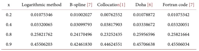
Table 3. Troesch’s problem with λ = 5.0 and h = 0.0005.

x Logarithmic method B-spline [7] Collocation[1] Doha [6] Fortran code [7]

0.2 0.01075346 0.01002027 0.00762552 0.01078872 0.01075342

0.4 0.03320065 0.03099793 0.03817903 0.03338672 0.03320051

0.8 0.25821762 0.24170496 0.23252435 0.25956596 0.25821664

[image:5.595.204.543.636.724.2]

[image:6.595.206.540.89.246.2]

DOI: 10.4236/am.2018.95039 555 Applied Mathematics

Table 4. Troesch’s problem with λ = 10 and h = 0.0005.

x Logarithmic method Temimi [8] Scott [10]

0.1 0.0000421216 0.0000421119 0.0000421118

0.2 0.0001299941 0.0001299641 0.0001299639

0.3 0.0003592878 0.0003589784 0.0003589779

0.4 0.0009781262 0.0009779027 0.0009779014

0.5 0.0026596252 0.0026590204 0.0026590172

0.6 0.0072305680 0.0072289310 0.0072289247

0.7 0.0196685008 0.0196640631 0.0196640603

0.8 0.0537425197 0.0537303294 0.0537303296

[image:6.595.207.543.275.713.2]

0.9 0.1521512477 0.1521140764 0.1521140787

Table 5. Troesch’s problem with λ = 60 and h = 0.0001.

x Logarithmic method Temimi [8]

0.1 0.0000000000 0.0000000000

0.6 0.0000000000 0.0000000000

0.8 0.0000004122 0.0000004096

0.9 0.0001663062 0.0001652505

0.95 0.0033431273 0.0033218844

0.97 0.0111942916 0.0111219726

0.98 0.0208631539 0.0207221628

0.99 0.0414467260 0.0411119440

1.0 1.0 1.0

[image:7.595.207.541.89.278.2]

DOI: 10.4236/am.2018.95039 556 Applied Mathematics

Table 6. Numerical solution using the logarithmic method and h = 0.0001.

λ = 100 λ = 150 λ = 200

x Logarithmic method x Logarithmic method x Logarithmic method

0.0 0.0000000000 0.0 0.0000000000 0.0 0.0000000000

0.8 0.0000000000 0.8 0.0000000000 0.8 0.0000000000

0.9 0.0000018373 0.9 0.0000000083 0.9 0.0000000000

0.95 0.0002726798 0.95 0.0000150234 0.95 0.0000009314

0.97 0.0020165050 0.98 0.0013534673 0.98 0.0003757441

0.98 0.0055113791 0.995 0.0139850466 0.995 0.0079377249

0.99 0.0156381379 0.998 0.0206481079 0.998 0.0168600022

0.999 0.0623708204 0.999 0.0362793031 0.999 0.0243867532

[image:7.595.207.540.307.496.2]

1.0 1.0 1.0 1.0 1.0 1.0

Table 7. Numerical solution using the logarithmic method and h = 0.0001.

λ = 300 λ = 1000

x Logarithmic method x Logarithmic method

0.0 0.0000000000 0.0 0.0000000000

0.8 0.0000000000 0.98 0.0000000000

0.9 0.0000000000 0.99 0.0000002099

0.95 0.0000000042 0.995 0.0000310894

0.97 0.0000017119 0.996 0.0000844853

0.98 0.0000343798 0.997 0.0002297760

0.99 0.0006910751 0.998 0.0006287443

0.995 0.0031516136 0.995 0.0018073693

1.0 1.0 1.0 1.0

Table 8. Numerical solution using Logarithmic method for large values of λ and h =

0.0001.

λ x Logarithmic method

104 _{0.9999 0.0009901753}

105 _{0.9999 0.0000760075}

106 _{0.9999 0.0000052983}

Table 9. Comparison of the proposed methods at λ = 0.9 with h = 0.0005.

λ Fourth order method Logarithmic method

0.5 0.8928542161 0.8928542162

1.0 0.8713625198 0.8713625212

5.0 0.4550600270 0.4550601074

[image:7.595.207.538.538.607.2] [image:7.595.208.539.639.724.2]

DOI: 10.4236/am.2018.95039 557 Applied Mathematics

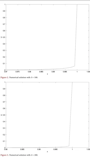
[image:8.595.153.536.55.722.2]

Figure 2. Numerical solution with λ = 100.

DOI: 10.4236/am.2018.95039 558 Applied Mathematics

[image:9.595.152.537.55.719.2]

Figure 4. Numerical solution with λ = 1000.

DOI: 10.4236/am.2018.95039 559 Applied Mathematics

4. Conclusion

In this work, we have derived a logarithmic finite difference method to over-come the difficulty in solving the Troesch’s problem for large values of λ. This progress is very important, since all existing methods were trying to obtain the numerical solution for Troesch’s problem for large values of λ. The logarithmic method which we have derived is able and succeeds to get the numerical solu-tion of Troesch’s problem for _{λ=0.5,5,10, ,10} 6_{. To recap things, a new}

loga-rithmic finite difference method is derived and can provide the numerical solu-tions for large values of λ. I think that, to the best of our knowledge, the method and some of the given results are published for the first time.

References

[1] El-Gamel, M. (2013) Numerical Solution of Troesch’s Problem by Sinc-Collocation Method. Applied Mathematics, 4, 707-712. https://doi.org/10.4236/am.2013.44098 [2] Feng, X., Mei, L. and He, G. (2007) An Efficient Algorithm for Solving Troesch’s

Problem. Applied Mathematics and Computation, 189, 500-507. https://doi.org/10.1016/j.amc.2006.11.161

[3] Erdogan, U. and Ozis, T. (2011) A Smart Nonstandard Finite Difference Scheme for Second Order Nonlinear Boundary Value Problems. Journal of Computational Physics, 230, 6464-6474. https://doi.org/10.1016/j.jcp.2011.04.033

[4] Deeba, E., Khuri, S.A.and Xie, S. (2000) An Algorithm for Solving Boundary Value Problems. Journal of Computational Physics, 159, 125-138.

https://doi.org/10.1006/jcph.2000.6452

[5] Temimi, H. (2012) A Discontinuous Galerkin Finite Element Method for Solving the Troesch’s Problem. Applied Mathematics and Computation, 219, 521-529. https://doi.org/10.1016/j.amc.2012.06.037

[6] Doha, E.H., Baleanu, D., Bahrawi, A.H. and Hafez, R.M. (2014) A Jacobi Colloca-tion Method for Tresch’s Problem in Plasma Physics. Proceedings of the Romanian Academy Series A, 15, 130-138.

[7] Khuri, S.A. and Sayfy, A. (2011) Troesch’s Problem: A B-Spline Collocation Ap-proach. Mathematical and Computer Modelling, 54, 1907-1918.

https://doi.org/10.1016/j.mcm.2011.04.030

[8] Temimi, H. and Kurkcu, H. (2014) An Accurate Asymptotic Approximation and Precise Numerical Solution of Highly Sensitive Troesch’s Problem. Applied Ma-thematics and Computation, 235, 253-260.

https://doi.org/10.1016/j.amc.2014.03.022

[9] El hajaji, A., Hilal, K., El Jalila, G. and El Mhamed, M. (2014) New Numerical Scheme for Solving Troesch’s Problem. Mathematical Theory and Modeling, 4, 65-72.