Comparison of Methods of Estimating Missing Values in Time Series

(1)

http://www.scirp.org/journal/ojs ISSN Online: 2161-7198

ISSN Print: 2161-718X

DOI: 10.4236/ojs.2018.82025 Apr. 30, 2018 390 Open Journal of Statistics

Comparison of Methods of Estimating Missing

Values in Time Series

I. S. Iwueze

1

, E. C. Nwogu

1

, V. U. Nlebedim

2*

, U. I. Nwosu

1

, U. E. Chinyem

1

1_{Department of Statistics, Federal University of Technology, Owerri, Nigeria} 2_{School of Mathematics and Statistics, University of Sheffield, Sheffield, UK}

Abstract

This paper proposes new methods of estimating missing values in time series data while comparing them with existing methods. The new methods are based on the row, column and overall averages of time series data arranged in a Buys-Ballot table with m rows and s columns. The methods assume that 1) only one value is missing at a time, 2) the trending curve may be linear, quad-ratic or exponential and 3) the decomposition method is either Additive or Multiplicative. The performances of the methods are assessed by comparing accuracy measures (MAE, MAPE and RMSE) computed from the deviations of estimates of the missing values from the actual values used in simulation. Results show that, under the stated assumptions, estimates from the new method based on full decomposition of a series is the best (in terms of the ac-curacy measures) when compared with other two new and the existing meth-ods.

Keywords

Missing Values, Buys-Ballot Table, Row and Column Averages, Row and Column Variances, Trend Parameters and Seasonal Indices

1. Introduction

The analysis of time series data constitutes an important area of statistics espe-cially in identifying the nature of the phenomenon represented by the sequence. However, missing observations in time series data are very common [1] [2]. This happens when an observation may not be made at a particular time, due to faulty equipment, lost records or a mistake, which cannot be rectified until later. When this happens, it is necessary to obtain estimates of the missing value for better understanding of the nature of the data and make possible a more accurate

fore-How to cite this paper: Iwueze, I.S., Nwogu, E.C., Nlebedim, V.U., Nwosu, U.I. and Chinyem, U.E. (2018) Comparison of Methods of Estimating Missing Values in Time Series. Open Journal of Statistics, 8, 390-399.

https://doi.org/10.4236/ojs.2018.82025

Received: August 3, 2017 Accepted: April 27, 2018 Published: April 30, 2018

http://creativecommons.org/licenses/by/4.0/

(2)

DOI: 10.4236/ojs.2018.82025 391 Open Journal of Statistics

cast [2].

In time series analysis, a problem frequently encountered in data collection is a missing observation. Missing observations may be virtually impossible to ob-tain, either because of time or cost constraints. In order to obtain estimates of these observations, there are different options available to the researcher. One of the options is to replace them by the mean of the series. The missing observation may be replaced with naive forecast or with the average of the last two known observations that bound the missing observation [3].

Using the Bode-Shannon representation of random processes and the “state-transition” method of analysis of dynamic systems, Kalman [4] worked on classical filtering and prediction in relation to missing values in time series. His work which hinged on state space modelling approach was later extended to ob-servational error and missing observations [Jones [5]]. Further on, Harvey and Pierse [6] highlighted on the relevance of state space modelling and Kalman fil-ter to the problems of missing data in times series. Their work discussed the maximum likelihood estimation of the parameters in an ARIMA model under missing observations and the estimation of missing observations. Using the uni-variate form of the modified Kalman filter, Kohn and Ansley [7] defined and computed efficiently the marginal likelihood of an ARIMA model with missing observations. Their work showed light on how to predict by interpolating miss-ing observations and obtainmiss-ing the mean squared error of the estimates.

As the literature reveals, missing values in time series has attracted so much research attention. Several approaches to determine missing values like the use of ARIMA models as well as other techniques have continued to evolve. Among them are the optimal linear combination of the forecast and back forecast method [Damsleth [8]], method for the estimation of models for discrete time series in the presence of missing data [Robinson and Dunsmuir [9]], forecasting techniques to estimate missing observations in time series [Abraham [10]], etc. A number of alternative procedures for estimating missing observations in stationary time series for autoregressive moving average models were provided by Ferreiro

[11]. Sequel to these alternative procedures in stationary time series, Rosen and Porat [12] introduced the general formulae for the asymptotic second-order mo-ments of the sample covariances, for missing values.

Another easily applicable spectral estimator for missing data is the method of Scargle [13]. This computes Fourier coefficients as the least squares fit of sines and cosines to the available remaining observations. The Lomb-Scargle spectrum is accurate in detecting strong spectral peaks but this assumption biases the de-scription of slopes and background shapes in the spectrum according to Bos et al.

[14] and Broersen et al. [15].

(3)

filtering.

Yuan et al. [17] compared the Normal-distribution-based maximum likeli-hood (ML) and multiple imputation (MI) procedures for analyzing missing value data. The paper compared these two procedures with respect to bias and efficiency of parameter estimates. Their result showed that ML is preferable to MI in practice, although parameter estimates by MI might still be consistent.

Cheema [18] compared different missing data handling methods (listwise de-letion, mean imputation, regression imputation, maximum likelihood imputa-tion and multiple imputaimputa-tion) using different methods of analysis (one sample t-test, two-sample t-test, two-way ANOVA and multiple regression). These methods, according to him are the four analytical methods that are frequently employed in educational research. However, his result did not cover handling missing values in time series data.

Indeed, procedures have been developed by statisticians to mitigate problems caused by missing data and various estimation methods have been reportedly used by different researchers to replace missing values [19] [20]. Briefly, the methods include mean imputation, series mean, mean of nearby points, median of nearby points, linear interpolation and Regression Imputations.

In time series, it is assumed that the data consist of observations made se-quentially in time; a systematic pattern (usually a set of identifiable components) and random noise (error). So, when some observations are missing it violets the condition for application of time series model. The systematic pattern includes the trend (denoted as Tt), seasonal (denoted as St) and the cyclical (denoted as

t

C) components. The random noise (or error, irregular component) is denoted

as It or et, where t stands for the particular point in time. These four classes

of time series components may or may not coexist in real-life data. These ponents can adopt different specific functional relationship. They can be com-bined in an additive (additive seasonality) or a multiplicative (multiplicative sea-sonality) fashion and can as well take other forms such as pseudo-additive/mixed (combining the elements of both the additive and multiplicative models) model. The Additive model, Multiplicative model and Pseudo-Additive/Mixed Model are given in Equations (1.1)-(1.3) respectively:

, 1, 2, ,

t t t t t

X = + +T S C +I t= n_(1.1)

, 1, 2, ,

t t t t t

X = × × ×T S C I t= n_(1.2)

, 1, 2, ,

t t t t t

X = × ×T S C +I t= n_(1.3)

Cyclical variation which refers to the long term oscillation or swings about the trend appears to an appreciable magnitude only in long period sets of data. However, if short period of time are involved (which is true of all examples of this study), the cyclical component is superimposed into the trend [21] hence, the trend-cycle component is denoted by Mt. In this case Equations (1.1)-(1.3),

may respectively, be written as:

, 1, 2, ,

t t t t

(4)

, 1, 2, ,

t t t t

X =M × ×S I t= n

_(1.5)

and

, 1, 2, ,

t t t t

X =M × +S I t= n

_(1.6)

The pseudo-additive model is used when the original time series contains very small or zero values. However, this work will discuss only the additive and multiplicative models.

Missing values can lead to erroneous conclusions about data. Substitution of missing values may introduce inaccuracies. It can lead to false results, forecast and errors or data skews can proliferate across subsequent runs causing a larger cumulative error effect. Most analytical methods cannot be performed if there are missing values in the data. Furthermore, existing methods did not consider the model structure (i.e. whether Additive or Multiplicative models) and other trending curves beyond the linear (Quadratic, Exponential etc.). More so, the seasonal component of the time series data was not taken into consideration in developing estimation methods as can be assessed from literature. Therefore the ultimate objective of this study is to develop methods of estimating missing val-ues which take into consideration the model structure and trending curve. The specific objectives are:

1) To review existing methods of estimating missing values. 2) Develop new methods of estimating missing values in time series 3) Assess the performance of the methods of estimating missing values. 4) Compare results from the existing methods of estimation of missing values with results from the new methods developed using simulated data.

Based on the results, recommendations are made.

The rationale for this study is to fill the gap in the existing methods of tion of missing values, by providing analyst with a better method for the estima-tion of missing values irrespective of model structure and funcestima-tional relaestima-tion- relation-ship.

2. Methodology

2.1. Existing Methods of Estimating Missing Values

The new methods proposed in this study assumed that the series are arranged in a Buys Ballot Table with m rows (periods) and s columns (seasons), for m>s.

Under this arrangement, the observation; Xt made at time t is identified by the

period i, (i=1, 2,,m) and season j, ( j=1, 2,,s) and t becomes

(t= −

(

i 1

)

s+ j). Thus, the observations in the i-th row (period) are

( )i1s1, ( )i1s2, , ( )i1s s

X _{− +} X _{− +} X _{− +} and the observations in the j-th column (season) are

( ) ( )

2 1 1

, , , , ,

j s j s j i s j m s j

X X + X + X − + X − + For details of the Buys Ballot table see

Iwu-eze and Nwogu [22] [23] and Iwueze et al. [24]. Therefore, for consistency, the existing methods have been presented using the Buys-Ballot format.

(5)

missing in the Buys-Ballot table at a point say t= −

(

i 1

)

s+ j, it is estimated

us-ing the different methods listed above as follows: 1) Mean Imputations (MI)

Mean imputation entails replacing the missing value with the mean of the values before the missing position. This is achieved by taking the summation of the val-ues and dividing by the number of observation before the missing position.

( )

_{( )}

( )

*

1 2 3

1 1 1 *

1

1 1

ˆ MI

1 1

n t

i s j i s j

t

X X X X X X

i s j n

− + − + −

=

 

= = _ + + + + _=

− + −

∑

(2.1)

where *

( )

1 1

n = −i s+ −j is the number of observations preceding the missing

observation.

2) Series Mean (SM)

Series mean estimates the missing value with the mean of the remaining series. Symbolically, the series mean is given by

( )

* . . 1

ˆ

SM ,

1 i s j

T X

n − +

= =

−

(2.2)

where, n=ms and

( ) ( )

*

. . 1 2 i1s j1 i1s j 1 ms

T =_X +X ++X ₋ _{+ −} +X ₋ _{+ +} ++X _

(2.3) 3) Linear Interpolation (LI)

This method of linear interpolation for estimating missing values is given by

( )1

(

( )1 1 ( )1 1

)

1 ˆ

LI

2

i s j i s j i s j

X _{− +} X _{− + −} X _{− + +}

= = +

_(2.4)

4) Regression Imputation (RI)

This method estimates the missing value by the estimate of the trend at the point of the missing value. Thus if the remaining values of the series are used to determine estimates of the trend parameters and the estimate of the missing value at

(

i−1

)

s+ j is given as:

a) For Linear Trend

( )1 ˆ

(

)

ˆ _ˆ

RI=X_i₋ _{s j}₊ = +a b_ i−1 s+ j_ (2.5)

b) For Quadratic Curve:

( )

(

)

(

)

2

1 ˆ

ˆ _ˆ _ˆ

RI=Xi− +s j = +a b i−1 s+ j+c i−1 s+ j

(2.6) c) For Exponential Curve:

( )1 ˆ ˆ(( )1 )

ˆ

RI=X_i₋ _{s j}₊ =bec i− s j+ (2.7)

2.2. New Methods of Estimating Missing Values

The new methods proposed in this work are the Row Mean Imputation, Column mean Imputation and Decomposition Without the Missing Value. The new methods are given as follows:

1) Row Mean Imputation (RMI)

(6)

the remaining observations in the row (period) containing the missing value. Thus, the missing value is estimated by

( ) ( ) ( )

1

1 1 1

1 1 1 ˆ RMI 1 j s

i s j i s u i s u

u u j

X X X

s − − + − + − + = = +   = = _ + _

− 

∑

(2.8)

2) Column Mean Imputation (CMI)

The columns mean imputation method computes estimate of the missing value as the mean of the remaining observations in the column (season) con-taining the missing value. Thus, the missing value is estimated as:

( ) ( ) ( )

1

1 1 1

1 1 1 ˆ CMI 1 i m

i s j u s j u s j

u u i

X X X

m − − + − + − + = = +   = = _ + _

− 

∑

 (2.9) 3) Decomposing Without the Missing Value (DWMV)

In this method, estimates of the trend parameters and seasonal indices ob-tained from the remaining observations using any of the methods of time series decomposition, are substituted into the expression for the missing value. Hence, the estimates of the missing values by this method are given by:

a) For Additive Model

( )1 ( )1 ˆ

ˆ ˆ

j

i s j i s j

X _{− +} =M _{− +} +S (2.10)

b) For the Multiplicative model.

( )1 ( )1 ˆ

ˆ ˆ

j

i s j i s j

X _{− +} =M _{− +} ×S

(2.11) The trend-cycle components of the DWMV method for the linear, quadratic and exponential curves are:

i) Linear Trend

( )1 ˆ

(

)

ˆ _ˆ ₁

i s j

M ₋ ₊ = +a b_ i− s+ j_

(2.12) ii) Quadratic Curve

( )

(

)

(

)

2

1 ˆ

ˆ _ˆ ₁ _ˆ ₁

i s j

M _{− +} = +a b_ i− s+ j_+c_ i− s+ j_ (2.13)

iii) Exponential Curve

( )1 ˆ ˆ( )1

ˆ _ec i s j

i s j

M ₋ ₊ =b  − +

(2.14)

2.3. Assessing Performance of the Methods

To assess the performance of our estimation methods, accuracy measures are computed from the deviations of the estimates of the missing values from the ac-tual values. The deviations of Xˆ( )i− +1s j from the Actual value X( )i− +1s j is given

as:

( )1 ( )1 ˆ( )1

ˆ_i _{s j} _i _{s j} _i _{s j}

e _{− +} =X _{− +} −X _{− +}

(7)

(Makridakis and Hibon, 1995). Given a data set of size n = ms, we considered one missing value at a time for different m0<n positions, n > 1. These

accu-racy measures are defined as follows: 1) Mean Absolute Error (MAE) The MAE is defined as

0

1 0

1 MAE

m

k k

e

m =

 

=  



∑

 (2.16)

2) Mean Absolute Percentage Error (MAPE) The MAPE is defined as:

0

1 0

1

MAPE 100

m k

k k

e

m = X

 

=_ _×

 



∑

 (2.17) 3) Root Mean Square Error (RMSE)

This is calculated as:

0

2

1 0

1 RMSE

m

k k

e

m =

=

∑

_(2.18)

3. Empirical Examples

This section presents some empirical examples to illustrate the application of the methods of estimating missing values discussed in Section 2. The empirical ex-ample consists of both simulated and real life data. The simulated series used consists of 106 data sets of 120 observations each simulated from the Additive model: Xt =Mt+ +St et, and Multiplicative model: Xt=Mt× ×St et, using the

MINITAB 16.0 version software. The trend-cycle component Mt used are 1)

Linear: Mt=

(

a+bt

)

with a = 1 and b = 2.0, 2) Quadratic:

2

t

M = + +a bt ct

with a = 1, b = 2.0 and c = 3 and 3) Exponential: M_t =bect with b = 10 and c =

0.02. In the Additive model, it is assumed that e_t ~N

( )

0,1 , while in the

Multi-plicative model, it is assumed that

( )

2

~ 1,

t

e N σ . The seasonal indices

, 1, 2, ,12

j

S j= are as shown in Table 1. The real life example used is the

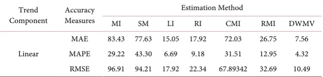
monthly time series data on Airline Passengers for the period of twenty (20) years. The summary of the accuracy measures for the seven methods of estimating miss-ing values considered are shown in Tables 2-4 for the selected trending curves.

The summary of accuracy measures for the simulated Additive and Multipli-cative models shown in Table 2 and Table 3 respectively indicates that DWMV has the lowest values of the accuracy measures (MAE, MAPE and RMSE) for all

Table 1. Seasonal indices used for simulation.

j 1 2 3 4 5 6 7 8 9 10 11 12

Sj (Add.) −0.89 −1.22 0.1 −0.15 −0.09 1.16 2.34 1.95 0.64 −0.73 −2.14 −0.97

Sj (Mult.) 0.91 0.88 1 0.98 0.98 1.12 1.26 1.2 1.05 0.92 0.8 0.9

(8)

[image:8.595.207.540.89.277.2]

Table 2. Summary result of estimation of missing value for additive model.

Trend

Component Accuracy Measures

Estimation Method

MI SM LI RI CMI RMI DWMV

Linear

MAE 67.03 62.29 7.07 11.26 63.96 11.89 2.59

MAPE 48.84 99.28 5.79 11.39 101.56 11.71 2.24

RMSE 76.77 68.53 9.70 14.59 73.46 16.58 3.29

Quadratic

MAE 10,335.21 10,591.89 819.45 982.11 8561.86 851.07 386.83

MAPE 66.44 524.74 5.66 10.75 437.68 17.55 2.74

RMSE 13,185.28 12,226.39 1221.91 1387.31 10171.44 1114.69 585.70

Exponential

MAE 21.61 22.07 2.37 3.43 20.74 4.24 1.03

MAPE 39.03 88.17 5.87 11.20 75.78 10.62 2.18

[image:8.595.207.540.307.494.2]

RMSE 28.03 26.09 3.17 4.37 24.03 5.25 1.54

Table 3. Summary result of estimation of missing value for multiplicative model.

Trend

Component Accuracy Measures

Estimation Method

Linear

MAE 61.43 55.92 1.25 36.17 63.95784 5.18 1.04

MAPE 48.65 87.54 1.37 29.48 105.4748 8.79 1.35

RMSE 69.55 64.69 1.54 39.91 74.2791 5.87 1.14

Quadratic

MAE 9653.18 10,511.27 3.12 1.47 18,576.20 851.07 1.07

MAPE 66.76 465.10 0.13 0.07 414.62 15.81 0.04

RMSE 12,547.42 12,120.50 3.48 1.87 388.72 1114.69 1.18

Exponential

MAE 20.03 22.05 1.25 1.42 18.47 2.25 0.95

MAPE 36.87 87.12 4.57 6.67 71.05 6.18 3.49

RMSE 26.81 26.14 1.54 1.82 21.62 3.10 1.08

Table 4. Summary result of estimation of missing value using the airline passenger data.

Trend

Component Measures Accuracy

Estimation Method

Linear

MAE 83.43 77.63 15.05 17.92 72.03 26.75 7.56

MAPE 29.22 43.30 6.69 9.18 31.51 12.95 4.32

RMSE 96.91 94.21 17.92 22.34 67.89342 32.69 10.49

[image:8.595.207.540.527.607.2]

(9)

seasonal effect in estimating the missing values. The information that DWMV takes into account seasonality of the missing value is supported by literature. For the real life data, the DWMV method also out-performed the other methods of estimation of missing values even as the assumption of normal distribution of error terms is not met in real life data.

4. Concluding Remark

The results of the analysis indicate that for all trending curves and both model structures, DWMV yielded best (in terms of the accuracy measures) estimates of the missing values when compared with both the existing methods and the two other new proposed methods (RMI and CMI). This is perhaps, because DWMV combines the effects of both the trending curves and the seasonal indices unlike the other methods. Cheema [18] also observed that multiple regression imputa-tion method of handling missing data performed well when the analytical method was multiple regression because using regression-imputed data in a re-gression equation was like fitting a rere-gression equation twice to predict the same dependent variable.

In view of this, it is recommended that the DWMV method be used in esti-mating missing values in time series analysis when one observation is missing at a time until further studies proves otherwise. It is also recommended that this study be extended to cases where more than one point data are missing at a time and to examine the effects of different sample sizes and distributions on the es-timation of missing values.

References

[1] David, S.C.F. (2006) Methods for the Estimation of Missing Values in Time Series.

Cowan University Press, Western Australia.

[2] Howell, D.C. (2007) The Analysis of Missing Data. In: Outhwaite, W. and Turner,

S., Eds., Handbook of Social Science Methodology, Sage, London.

https://doi.org/10.4135/9781848607958.n11

[3] Almed, M.R. and Al-Khazaleh, A.M.H. (2008) Estimation of Missing Data by Using

the Filtering Process in a Time Series Modeling.

[4] Kalman, R.E. (1960) A New Approach to Linear Filtering and Prediction Problems.

Journal of Basic Engineering, 81, 35-45. https://doi.org/10.1115/1.3662552

[5] Jones, R.H. (1980) Maximum Likelihood Fitting of ARMA Models to Time Series

with Missing Observations. Technimetrics, 22, 389-395.

https://doi.org/10.1080/00401706.1980.10486171

[6] Harvey, A.C. and Pierse, R.G. (1984) Estimating Missing Observations in Economic

Time Series. Journal of the American Statistical Association,79, 125-131.

https://doi.org/10.1080/01621459.1984.10477074

[7] Kohn, R. and Ansley, C.F. (1986) Estimation, Prediction, and Interpolation for

ARIMA Models with Missing Data. Journal of the American Statistical Association,

81, 751-761. https://doi.org/10.1080/01621459.1986.10478332

[8] Damsleth, E. (1979) Interpolating Missing Values in a Time Series. Scand Journal of

(10)

[9] Robinson, P.M. and Dunsmuir, W. (1981) Estimation of Time Series Models in the

Presence of Missing Data. Journal of the American Statistical Association, 76,

560-568. https://doi.org/10.1080/01621459.1981.10477687

[10] Abraham, B. (1981) Missing Observations in Time Series. Communications in

Sta-tistics Theory A,10, 1643-1653. https://doi.org/10.1080/03610928108828138

[11] Ferreiro, O. (1987) Methodologies for the Estimation of Missing Observations in

Time Series. Statistics and Probability Letters, 5, 65-69.

https://doi.org/10.1016/0167-7152(87)90028-9

[12] Rosen, Y. and Porat, B. (1989) Optimal ARMA Parameter Estimation Based on the

Sample Covariances for Data with Missing Observations. IEEE Transactions on

In-formation Theory, 35, 342-349. https://doi.org/10.1109/18.32128

[13] Scargle, J.D. (1982) Studies in Astronomical Time Series Analysis II. Statistical

As-pects of Spectral Analysis of Unevently Spaced Data. Astrophysics Journal, 263,

836-853.

[14] Bos, R., De walele, S. and Broersen, M.T.P. (2002) Autoregressive Spectral Estimates

by Application of the Burg Algorithm to Irregularly Sampled Data. IEEE

Transac-tion on Instrument and Measurement, 51, 1289-1294.

https://doi.org/10.1109/TIM.2002.808031

[15] Broersen, M.T.P., De Waele, S. and Bos, R. (2004) Autoregressive Spectral Analysis

When Observation Are Missing. Automatica, 40, 1495-1504.

https://doi.org/10.1016/j.automatica.2004.04.011

[16] Brockwell, P.J. and Davis, R.A. (1991) Time Series: Theory and Methods.

Springer-Verlag, New York. https://doi.org/10.1007/978-1-4419-0320-4

[17] Yuan, K.H., Yang-Wallentin, F. and Bentler, P.M. (2012) Maximum Likelihood

versus Multiple Imputation for Missing Data with Violation of Distribution Condi-tion. Sociological Methods & Research, 41, 598-629.

[18] Cheema, J.R. (2014) Some General Guidelines for Choosing Missing Data Handling

Methods in Educational Research. Journal of Modern Applied Statistical Methods,

13, Article 3. https://doi.org/10.22237/jmasm/1414814520

[19] Schafer, J.L. (1997) Analyses of Incomplete Multivariate Data. Chapman and Hall,

New York. https://doi.org/10.1201/9781439821862

[20] Witta, E.L. (2000) Effectiveness of Four Methods of Handling Missing Data Using

Samples from a National Database. Paper Presented at the Annual Meeting of the

American Educational Research Association, ERIC Document Reproduction Ser-vice No. ED 442 810, New Orleans, LA.

[21] Chatfield, C. (2004) The Analysis of Time Series: An Introduction. 6th Edition,

Chapman and Hall, London.

[22] Iwueze, I.S. and Nwogu, E.C. (2004) Buys-Ballot Estimates for Time Series

Decom-position. Global Journal of Mathematics, 3,83-98.

[23] Iwueze, I.S and Nwogu, E.C. (2005) Buys-Ballot Estimates for Exponential and

S-Shaped Curves, for Time Series. Journal of the Nigerian Association of

Mathe-matical Physics, 9, 357-366.

[24] Iwueze, S.I., Nwogu, E.C., Ohakwe, J. and Ajaraogu, J.C. (2011) Uses of the

Buys-Ballot Table in Time Series Analysis. Applied Mathematics, 2, 633-645.