On Recoverable and Two-Stage Robust
Selection Problems with Budgeted
Uncertainty
Andr´
e Chassein
1, Marc Goerigk
2, Adam Kasperski
3, and Pawe l
Zieli´
nski
41Fachbereich Mathematik, Technische Universit¨at Kaiserslautern, Germany 2Department of Management Science, Lancaster University, United Kingdom 3Faculty of Computer Science and Management, Wroc law University of Science and
Technology, Poland
4Faculty of Fundamental Problems of Technology, Wroc law University of Science and
Technology, Poland
July 31, 2017
Abstract
In this paper the problem of selecting p out of n available items is discussed, such that their total cost is minimized. We assume that the item costs are not known exactly, but stem from a set of possible outcomes modeled through budgeted uncertainty sets, i.e., the interval uncertainty sets with an additional linear (bud-get) constraint, in their discrete and continuous variants. Robust recoverable and two-stage models of this selection problem are analyzed through an in-depth dis-cussion of variables at their optimal values. Polynomial algorithms for both models under continuous budgeted uncertainty are proposed. In the case of discrete bud-geted uncertainty, compact mixed integer formulations are constructed and some approximation algorithms are proposed. Polynomial combinatorial algorithms for the adversarial and incremental problems (the special cases of the considered robust models) under both discrete and continuous budgeted uncertainty are constructed.
Keywords: combinatorial optimization; robust optimization; selection problem; budgeted uncertainty; two-stage robustness; recoverable robustness
1 Introduction
In this paper we consider the following Selection problem. We are given a set of n
X ⊆ [n] of p items, |X| = p, whose total cost P
i∈Xci is minimum. It is easy to see that an optimal solution is composed ofp items of the smallest cost. It can be found in
O(n) time by using the well-known fact, that thepth smallest item can be found inO(n) time (see, e.g., [11]). Selectionis a basic resource allocation problem [18]. It is also a
special case of 0-1 knapsack, 0-1 assignment, single machine scheduling, and minimum matroid base problems (see [20] for an overview). It can be formulated as the following integer linear program:
min P
i∈[n]cixi s.t. P
i∈[n]xi =p
xi ∈ {0,1} ∀i∈[n].
(1)
We will use Φ ⊆ {0,1}n to denote the set of all feasible solutions to (1). Given xxx ∈ {0,1}n, we also define X
x x
x ={i∈[n] : xi = 1}, and Xxxx = [n]\Xxxx, i.e. Xxxx is the item set induced by vectorxxx and Xxxx denotes its complement.
Consider the case when the item costs are uncertain. As a part of the input, we are given a scenario setU, containing all possible vectors of the item costs, calledscenarios. Several methods of definingU have been proposed in the existing literature (see, e.g., [3, 4, 19, 24, 27]). Under discrete uncertainty (see, e.g., [24]), the scenario set contains K
distinct scenarios i.e. UD = {ccc
1, . . . , cccK}, ccci ∈ Rn+. Under interval uncertainty, the cost of each item i ∈ [n] belongs to a closed interval [ci, ci], where di := ci−ci ≥ 0 is the maximal deviation of the cost of i from its nominal value ci. In the traditional interval uncertainty representation, UI is the Cartesian product of all the intervals (see, e.g., [24]). In this paper we will focus on the following two generalizations of scenario setUI, which have been examined in [3, 4, 27]:
• Continuous budgeted uncertainty:
Uc={(c
i+δi)i∈[n]:δi ∈[0, di], X
i∈[n]
δi ≤Γ} ⊆Rn+.
• Discrete budgeted uncertainty:
Ud={(ci+δi)i∈[n]:δi∈ {0, di},|{i∈[n] :δi=di}| ≤Γ} ⊆Rn+.
The fixed parameter Γ≥0 is called a budget and it controls the amount of uncertainty which an adversary can allocate to the item costs. For a sufficiently large Γ,Ucreduces toUI, and Udreduces to the extreme points of UI.
In order to compute a solution, under a specified scenario set U, we can follow a robust optimization approach. For general overviews on robust optimization, see, e.g., [1, 15, 22, 24, 28]. In a typical, single-stage robust model we seek a solution minimizing the total cost in a worst case. This leads to the following minmax and minmax regret
problems:
MinMax: min
x x
x∈Φmaxccc∈U cccxxx,
MinMax-Regret: min
x
The minmax (regret) versions of the Selection problem have been discussed in the
existing literature. For scenario setUD both problems are NP-hard even forK= 2 (the number of scenarios equals 2) [2]. IfKis part of the input, thenMinMaxand
MinMax-Regretare strongly NP-hard and not approximable within any constant factor [20]. On
the other hand,MinMaxis approximable withinO(logK/log logK) [13] but
MinMax-Regret is only known to be approximable withinK, which is due to the results given
in [1]. The MinMax problem under scenario sets Uc and Ud is polynomially solvable,
according to the results obtained in [3]. Also,MinMax-Regret, under scenario setUI,
is polynomially solvable by the algorithms designed in [2, 10].
The problems which arises in practice often have a two-stage nature. Namely, a partial solution is computed in the first stage and completed in the second stage, or a complete solution is formed in the first stage and modified to some extent in the second stage. Typically, the costs in the first stage are precisely known, while the costs in the second stage are uncertain. Before we formally define the two-stage models, let us introduce some additional notation:
• Φ1={xxx∈ {0,1}n:Pi∈[n]xi≤p},
• Φxxx={yyy∈ {0,1}n:Pi∈[n](xi+yi) =p, xi+yi≤1, i∈[n]}, xxx∈Φ1,
• Φk x
xx={yyy∈ {0,1}n: P
i∈[n]yi=p, Pi∈[n]xiyi ≥p−k}, xxx∈Φ, k∈[p]∪ {0}. Ifyyy ∈Φxxx, thenXxxx∩Xyyy =∅and|Xxxx∪Xyyy|=p. Hence Φxxxencodes all subsets of the item set [n], which added to Xxxx form a complete solution of cardinality p. Set Φxxkx is called a
recovery set,kis a givenrecovery parameter. Ifyyy∈Φkxxx, then|Xxxx\Xyyy|=|Xyyy\Xxxx| ≤k, so Φkxxx encodes all solutions which can be obtained fromXxxx by exchanging up tokitems. LetCCC = (C1, . . . , Cn) be a vector of the first stage item costs, which are assumed to be precisely known. Let scenario setU contain all possible vectors of the uncertain second stage costs. Given k ∈ [p]∪ {0}, we study the following robust recoverable selection
problem:
RREC: min
xxx∈Φ
C
CCxxx+ max ccc∈U yyy∈minΦk
x x x
cccyyy
. (2)
InRREC a complete solution (exactlypitems) is chosen in the first stage. Then, after
a scenario fromU reveals, one can exchange optimally up tokitems in the second stage. Notice that if k = 0 and Ci = 0 for each i ∈ [n], then RREC becomes the MinMax problem. The robust recoverable model for linear programming, together with some applications, was discussed in [25]. It has been also recently applied to the shortest path [5], spanning tree [16, 17], knapsack [6] and traveling salesman problems [8]. The
RREC problem under scenario sets UD and UI has been recently discussed in [21].
Under UD it turned out to be NP-hard for constant K, strongly NP-hard and not at all approximable when K is part of the input (this is true even if k= 1). On the other hand, under scenario set UI, a polynomial O((p−k)n2) time algorithm for
RREC has
We also analyze the following robust two-stage selection problem:
R2ST: min
xxx∈Φ1
C
CCxxx+ max ccc∈U yyy∈minΦxxx
cccyyy
, (3)
In R2ST we seek a first stage solution, which may contain less than p items. Then,
after a scenario from U reveals, this solution is completed optimally to p items. The robust two-stage model was introduced in [23] for the bipartite matching problem. The R2ST problem has been recently discussed in [21]. It is polynomially solvable under scenario setUI. For scenario setUD, the problem becomes strongly NP-hard and it has an approximability lower bound of Ω(logn), but it has an O(logK+ logn) randomized approximation algorithm. No results for scenario sets Uc and Ud have been known to date.
Given a first stage solution xxx ∈ Φ (resp. xxx ∈ Φ1), we will also study the following
adversarial problems:
AREC: max
ccc∈U yyy∈minΦk x x x
cccyyy, (4)
A2ST: max
ccc∈U yyy∈minΦxxx
cccyyy. (5)
If, additionally, scenarioccc∈ U is fixed, then we get the followingincremental problems:
IREC: min
y yy∈Φk
x x x
cccyyy, (6)
I2ST: min
y yy∈Φxxx
cccyyy. (7)
The adversarial and incremental versions of some network problems were discussed in [12, 27]. The incremental versions of the shortest path and the spanning tree problems are polynomially solvable [12], whereas the adversarial versions of these problems under scenario setUd are strongly NP-hard [14, 26, 27].
A summary of the results forUD and UI obtained in [21] is presented in Table 1.
Table 1: The known results for UD and UI obtained in [21].
U IREC AREC RREC I2ST A2ST R2ST
O(n) O(Kn) NP-hard for const. K; O(n) O(Kn) NP-hard for const. K;
str. NP-hard str. NP-hard
UD not at all appr. appr. inO(logK+ logn)
for unboundedK Ω(logn) approximability lower bound
for unboundedK UI O(n) O(n) O((p−k)n2) O(n) O(n) O(n)
polynomially solvable under scenario set Uc. The polynomial algorithms for
RREC
and R2ST under Uc are based on solving a polynomial number of linear programming
subproblems. We also provide polynomial time combinatorial algorithms for AREC
and A2ST under both Uc and Ud. The complexity of RREC and R2ST under Ud
remains open. For these problems we construct compact MIP formulations and propose approximation algorithms. To achieve these results, we provide an in-depth analysis of
Table 2: New results forUc and Ud shown in this paper.
U IREC AREC RREC I2ST A2ST R2ST
Uc O(n) O(n2) poly. sol. O(n) O(n2) poly. sol.
O(nlogn) compact MIP O(nlogn) compact MIP Ud O(n) O(n3) compact MIP O(n) O(n2) compact MIP
problem variables at optimality. In itself, this is a key contribution facilitating the un-derstanding of our models, providing insight to a decision maker, and giving an intuitive interpretation of the problem complexity.
2 Continuous Budgeted Uncertainty
In this section we address the recoverable and two-stage robust selection problems,
RREC (2) and R2ST (3), under the continuous budgeted uncertainty Uc. We first
consider the incremental and adversarial problems,IREC(6) andAREC(4), which are
inner ones of RREC. We will show thatIRECcan be solved inO(n) time. TheAREC
is more involved problem for which we will build a nontrivialO(n2) algorithm (its com-plexity can be reduced to O(nlogn), if we apply more clever data structure). Finally, we will show that RREC can be solved in polynomial time. We then investigate the
two-stage setting. In order to solve the incremental and adversarial problems,I2ST(7) andA2ST(5), we will apply the results obtained forIRECandAREC and provide for
both problemsO(n) and O(n2) algorithms, respectively. We will finish by showing that
R2STcan be solved in polynomial time.
2.1 Recoverable Robust Selection
2.1.1 The incremental problem
Givenxxx∈Φ andccc∈ U, the incremental problem,IREC (6), can be formulated as the
following linear program (notice that the constraints yi∈ {0,1}can be relaxed):
opt1= min X
i∈[n]
ciyi
s.t. X
i∈[n]
yi =p
X
i∈[n]
xiyi≥p−k
yi ∈[0,1] i∈[n]
It is easy to see that the IREC problem can be solved in O(n) time. Indeed, we first
choose p−k items of the smallest cost from Xxxx and then k items of the smallest cost from the remaining items. We will now show some additional properties of (8), which will be used extensively later. The dual to (8) is
max pα+ (p−k)β−X i∈[n]
γi
s.t. α+xiβ ≤γi+ci i∈[n]
β ≥0
γi≥0 i∈[n]
(9)
From now on, we will assume that k >0 (the casek= 0 is trivial, sinceyyy=xxx holds). Letb(ccc) be thepth smallest item cost for the items in [n] underccc(i.e. ifcσ(1) ≤ · · · ≤cσ(n) is the ordered sequence of the item costs underccc, thenb(ccc) =cσ(p)). Similarly, letb1(ccc) be the (p−k)th smallest item cost for the items inXxxxandb2(ccc) be thekth smallest item cost for the items in Xxxx under ccc. The following proposition characterizes the optimal values ofα and β in (9), and is fundamental in the following analysis:
Proposition 1. Given scenarioccc∈ U, the following conditions hold:
1. if b1(ccc)≤b(ccc), then α=b(ccc) andβ = 0 are optimal in (9),
2. if b1(ccc)> b(ccc), then α=b2(ccc) andβ =b1(ccc)−b2(ccc) are optimal in (9).
Proof. By replacing γi by [α+βxi−ci]+, the dual problem (9) can be represented as follows:
max
α,β≥0f(α, β) = maxα,β≥0
pα+ (p−k)β−X i∈[n]
[α+βxi−ci]+
, (10)
where [a]+ = max{0, a}. Let us sort the items in [n] so that that cσ(1) ≤ · · · ≤ cσ(n). Let us sort the items in Xxxx so that cν(1) ≤ · · · ≤ cν(p) and the items in Xxxx so that
cς(1) ≤ · · · ≤cς(n−p). We distinguish two cases. The first one: cν(p−k) ≤ cσ(p) (b1(ccc) ≤
b(ccc)). Then it is possible to construct an optimal solution to (8) with the cost equal to P
i∈[p]cσ(i). Namely, we choosep−k items of the smallest costs from Xxxx and k items of the smallest cost from the remaining items. Fix α=cσ(p) and β= 0, which gives the case 1. By using (10), we obtainf(α, β) =P
i∈[p]cσ(i)=opt1and the proposition follows from the weak duality theorem. The second case: cν(p−k) > cσ(p) (b1(ccc) > b(ccc)). The optimal solution to (8) is then formed by the itemsν(1), . . . , ν(p−k) andς(1), . . . , ς(k). Fixα=cς(k) and β =cν(p−k)−cς(k), which gives the case 2. By (10), we have
f(α, β) =pα+ (p−k)β− X i∈Xxxx
[α+β−ci]+− X
i∈Xxxx
[α−ci]+
=pcς(k)+ (p−k)(cν(p−k)−cς(k))− X
i∈Xxxx
[cν(p−k)−ci]+− X
i∈Xxxx
[cς(k)−ci]+
=pcς(k)+ (p−k)(cν(p−k)−cς(k))−(p−k)cν(p−k)+ X
i∈[p−k]
cν(i)−kcς(k)+X i∈[k]
= X i∈[p−k]
cν(i)+ X
i∈[k]
cς(i) =opt1
and the proposition follows from the weak duality theorem.
2.1.2 The adversarial problem
Consider the adversarial problem AREC (4) for a given solution xxx ∈Φ. We will again
assume that k > 0. If k = 0, then all the budget Γ is allocated to the items in Xxxx. Scenario ccc∈ Uc which maximizes the objective value in this problem is called a worst
scenario for xxx (worst scenario for short). We now give a characterization of a worst scenario.
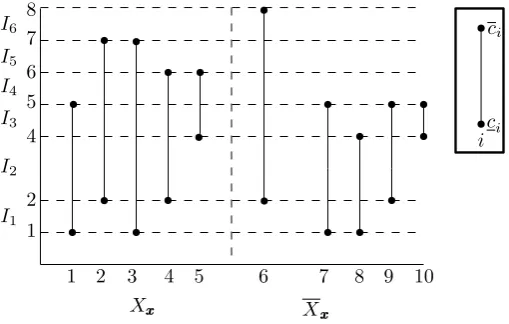
Proposition 2. There is a worst scenarioccc= (ci+δi)i∈[n]∈ Uc such that
1. b1(ccc)≤b(ccc) or
2. b1(ccc) or b2(ccc) belongs toD={c1, . . . , cn, c1, . . . , cn}.
Xxxx Xxxx
1 2 3 4 5 6 7 8 9 10
c i ci
i δi
Xxxx Xxxx
1 2 3 4 5 6 7 8 9 10
±∆
3
±∆3
±∆
3
±∆2
±∆
2
a) b)
+∆
−∆
3
−∆
3 −∆
3
b1(c) b1(c)
b2(c) b2(c)
+∆
−∆
2
−∆
[image:7.595.91.507.311.478.2]2
Figure 1: Illustration of the proof forn= 10,p= 5,k= 2, andXxxx={1, . . . ,5}.
Proof. Let ccc be a worst scenario and assume that b1(ccc) > b(ccc) and both b1(ccc) and
b2(ccc) do not belong to D. The idea of the proof is to show that there is also a worst scenario satisfying condition 1 or 2. Note that b1(ccc) > b(ccc) implies b1(ccc) > b2(ccc). Let
A={i∈Xxxx :ci+δi =b1(ccc)}andB={i∈Xxxx :ci+δi =b2(ccc)}. Observe thatA, B 6=∅ by the definition of b1(ccc) and b2(ccc). Also, a positive budget must be allocated to each item in A and B. In Figures 1a and 1b we have A = {2,4,5} and B ={7,9}. Let k1 be the number of items in Xxxx such that ci+δi < b1(ccc) and k2 be the number of items inXxxx such thatci+δi < b2(ccc). In the sample problem (see Figures 1a and 1b) we have
δi−∆/|A| ≥0 for each i∈ A. Letyyy be an optimal solution under ccc and letyyy1 be an optimal solution underccc1. The following equality holds
ccc1yyy1 =cccyyy+ ∆−(p−k−k1) ∆ |A|.
Since |A|+k1 ≥ p−k, ccc1yyy1 ≥ cccyyy and ccc1 is also a worst scenario. We can increase ∆ so that the condition 1 or 2 of the proposition is satisfied, or b1(ccc1) = cj +δj, or
cj +δj = cj +dj (see Figure 1a). The same reasoning can be applied to every item
j ∈ Xxxx such that cj +δj < b2(ccc) and δj < dj (see the item 8 in Figure 1a). So, it remains to analyze the case shown in Figure 1b. Let us again choose some sufficiently small ∆ > 0. Define scenario ccc1 by modifyingccc in the following way δi := δi+ ∆/|A| for each i ∈ A and δi := δi−∆/|B| for each i ∈ B. Similarly, define scenario ccc2 by modifying ccc as follows δi := δi−∆/|A| for each i ∈ A and δi := δi+ ∆/|B| for each
i∈B. Letyyy1 be an optimal solution underccc1 andyyy2 be an optimal solution underccc2. The following equalities hold
ccc1yyy1 =cccyyy+ (p−k−k1) ∆
|A|−(k−k2) ∆ |B|,
ccc2yyy2 =cccyyy−(p−k−k1) ∆
|A|+ (k−k2) ∆ |B|.
Hence, eitherccc1yyy1 ≥cccyyy orccc2yyy2 ≥cccyyy, so ccc1 orccc2 is also a worst scenario. We can now increase ∆ untilccc1 (ccc2) satisfies condition 1 or 2.
Using (9) and the definition of scenario setUc, we can represent
ARECas the following
linear programming problem:
max pα+ (p−k)β−P i∈[n]γi
s.t. α+xiβ ≤γi+ci+δi ∀i∈[n] P
i∈[n]δi ≤Γ
δi≤di ∀i∈[n]
β≥0
γi, δi≥0 i∈[n]
(11)
Thus AREC can be solved in polynomial time. In the following we will construct
a strongly polynomial combinatorial algorithm for solvingAREC. The following
corol-lary is a consequence of Proposition 1 and Proposition 2:
Corollary 3. There is an optimal solution to (11) in which
1. β = 0 or
Proof. According to Proposition 1, there is an optimal solution to (11) which induces a worst scenarioccc= (ci+δi)i∈[n]∈ Uc, which satisfies conditions 1 and 2 of Proposition 1. If the condition 1 is fulfilled, i.e. b1(ccc) ≤ b(ccc), then according to Proposition 2 we get β = 0. If b1(ccc) > b(ccc), then condition 2 from Proposition 1 and condition 2 from Proposition 2 hold. Both these conditions imply the condition 2 of the corollary.
Proposition 4. The optimal values of α and β in (11) can be found by solving the following problem: max α,β≥0
αp+β(p−k)−max
X
i∈[n]
[α+βxi−ci]+−Γ, X
i∈[n]
[α+βxi−ci]+ (12)
Proof. Let us first rewrite (11) in the following way:
max pα+ (p−k)β−X i∈[n]
[α+βxi−ci−δi]+
s.t. X i∈[n]
δi ≤Γ
0≤δi≤di i∈[n]
β≥0
(13)
Let us fix α and β ≥ 0 in (13). Then the optimal values of δi can be then found by solving the following subproblem:
z= min X i∈[n]
[α+βxi−ci−δi]+
s.t. X i∈[n]
δi ≤Γ
0≤δi≤di i∈[n]
(14)
Let U =P
i∈[n][α+βxi−ci]+. Observe that [U −Γ]+ is a lower bound on z asz ≥0 and it is not possible to decreaseU by more than Γ. The subproblem (14) can be solved by applying the following greedy method. For i= 1, . . . , n, if α+βxi −ci > 0, we fix
δi = min{α+βxi−ci, di,Γ} and modify Γ := Γ−δi. If, at some step, Γ = 0 we have reached the lower bound. Hencez= [U−Γ]+. On the other hand if, after the algorithm terminates, we still have Γ>0, then z=P
i∈[n][α+βxi−ci−di]+. In consequence
z= max
[U−Γ]+, X
i∈[n]
[α+βxi−ci−di]+ = max X
i∈[n]
[α+βxi−ci]+−Γ, X
i∈[n]
[α+βxi−ci]+
,
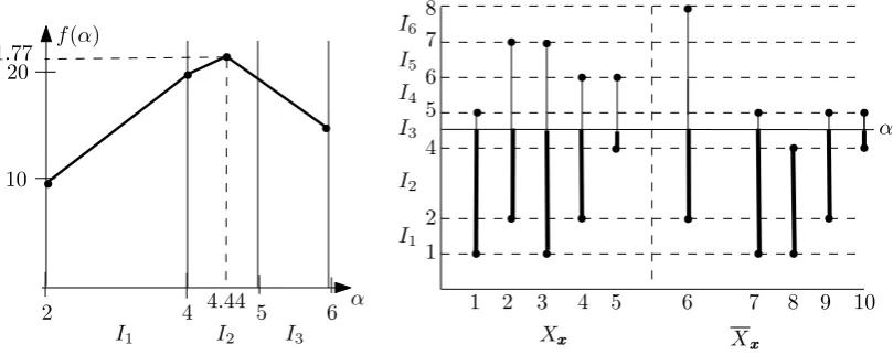
Having the optimal values of α and β, the worst scenario ccc = (ci+δi)i∈[n], can be found in O(n) time by applying the greedy method to (14), described in the proof of Proposition 4. We now construct an efficient algorithm for solving (12), which will give us the optimal values of α and β. We will illustrate this algorithm by using the sample problem shown in Figure 2.
I1 I2 I3 I4 I5 I6
ci ci
i
Xxxx Xxxx
1 2 3 4 5 6 7 8 9 10
[image:10.595.171.426.163.325.2]1 2 4 5 6 7 8
Figure 2: A sample problem withn= 10, p= 5,k= 2, Γ = 24, andXxxx={1, . . . ,5}.
Let h(1) ≤ h(2) ≤ · · · ≤ h(l) be the ordered sequence of the distinct values from D. This sequence defines a family of closed intervals Ij = [h(j), h(j+1)], j ∈ [l−1], which partitions the interval [mini∈[n]ci,maxi∈[n]ci]. Notice thatl≤2n. In the example shown in Figure 2 we have six intervals I1, . . . I6 which split the interval [1,8].
By Corollary 3, we need to investigate two cases. In the first case, we have β = 0. Then (12) reduces to the following problem:
max
α f(α) = maxα
αp−max
X
i∈[n]
[α−ci]+−Γ, X
i∈[n]
[α−ci−di]+
. (15)
Consider the problem of maximizing f(α) over a fixed interval Ij. It is easy to verify that (15) reduces then to finding the maximum of a minimum of two linear functions of α over Ij. For example, when α ∈ I3 = [4,5], then after an easy computation, the problem (15) becomes
max α∈[4,5]
min{−5α+ 44,4α+ 4}.
sample problem is shown in Figure 2. The optimal value of α is 4.44. The scenario corresponding to α = 4.44 can be obtained by applying a greedy method and it is also shown in Figure 3.
2 4 5 6
10 20
4:44 21:77
α f(α)
I1
I2
I3
I4
I5
I6
Xxxx Xxxx
1 2 3 4 5 6 7 8 9 10
1 2 4 5 6 7 8
α
[image:11.595.99.504.137.298.2]I1 I2 I3
Figure 3: The function f(α) for the sample problem and the worst scenario for the optimal value of α= 4.44.
We now discuss the second case in Corollary 3. Let us fixγ =α+β and rewrite (12) as follows:
max
α,γ≥αg(α, γ) = maxα,γ≥α{αk+γ(p−k)−
max
X
i∈Xxxx
[γ−ci]++ X
i∈Xxxx
[α−ci]+−Γ, X
i∈Xxxx
[γ−ci−di]++ X
i∈Xxxx
[α−ci−di]+
.
(16) According to Corollary 3, the optimal value of α orγ belongs toD. So, let us first fix
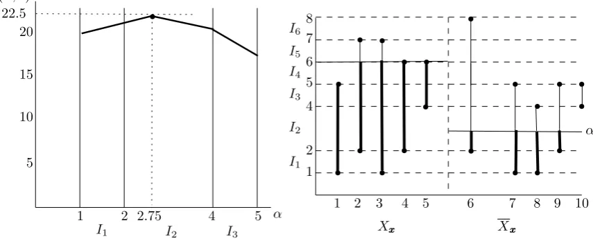
γ ∈ D and consider the problem maxαg(α, γ). The optimal value ofα can be found by optimizing α over each interval Ij, whose upper bound is not greater then γ (it follows from the constraint α ≤ γ). Again, the problem maxα∈Ijg(α, γ) can be reduced to
maximizing a minimum of two linear functions of α over a closed interval. To see this consider the sample problem shown in Figure 2. Fix γ = 6 and assume that α ∈ I2. Then, a trivial verification shows that
max
α∈[2,4]g(α,6) = maxα∈[2,4]min{28−2α,2α+ 17}.
The maximum is attained when 28−2α = 2α+ 17, so for α = 2.75. The function
1 2 4 5 5
10 15 20 22:5
I1 I2 I3 I4 I5 I6
Xxxx Xxxx
1 2 3 4 5 6 7 8 9 10
1 2 4 5 6 7 8
α
2:75 α
g(α;6)
[image:12.595.96.524.93.267.2]I1 I2 I3
Figure 4: The function g(α,6) for the sample problem and the worst scenario for the optimal value of α= 2.75.
We can then repeat the reasoning for every fixedα∈ D. Namely, we solve the problem maxγ≥αg(α, γ) by solving the problem for each interval whose lower bound is not less thanα. Again, not all values ofα∈ D need to be examined. Sinceαis thekth smallest item cost inXxxx, we should check only the values ofα∈ {1,2,4,5}.
Theorem 5. The problem AREC under scenario set Uc can be solved in O(n2) time.
Proof. We will present a sketch of the O(n2) algorithm. We first determine the family of intervals I1, . . . , Il, which requiresO(nlogn) time. Now, the key observation is that we can evaluate first all the sums that appear in (15) and (16) for each interval Ij. We can compute and store these sums for every Ij in O(n2) time. Now each problem maxα∈Ijg(α, γ) for γ ∈ D, maxγ∈Ijg(α, γ) for α ∈ D, and maxα∈Ijf(α) can be solved
in constant time by inserting the computed earlier sums into (16) and (15). The number of problems that must be solved is O(n2), so the overall running time of the algorithm isO(n2).
Using a more refined analysis and data structures such as min-heaps (see, e.g., [11]), thisO(n2) result can be further improved toO(nlogn). The detailed proof can be found in the technical report of this paper (see [9]).
We now show the following proposition, which will be used later:
Proposition 6 (Dominance rule). Let k, l be two items such thatck≤cl and ck≤cl.
Let xl = 1 and xk = 0 in (11). Then the maximum objective value in (11) will not
increase when we changexl= 0 and xk = 1.
Proof. Let Xxxx0 = Xxxx ∪ {k} \ {l}. Notice that (15) does not depend on the first stage
enough to show that for eachα and γ ≥α the following inequalities hold:
U1= [γ−ck]+−[γ−cl]++ [α−cl]+−[α−ck]+≥0 (17)
and
U2 = [γ−ck]+−[γ−cl]++ [α−cl]+−[α−ck]+ ≥0. (18) Inequality (17) can be proven by distinguishing the following cases: if α≤γ ≤ck≤cl, then U1 = 0; if α ≤ ck ≤ γ ≤ cl, then U1 = γ −ck ≥ 0; if α ≤ ck ≤ cl ≤ γ, then
U1 = cl−ck ≥ 0; if ck ≤α ≤γ ≤ cl, then U1 = γ−α ≥ 0; if ck ≤ α ≤ cl ≤ γ, then
U1 =γ −ck−γ+cl−α+ck =cl−α≥0; ifck ≤cl ≤α ≤γ, then U1 = 0. The proof of the fact thatU2≥0 is just the same.
2.1.3 The recoverable robust problem
In this section we studyRREC(2) under scenario setUc. We first identify some special
cases of this problem, which are known to be polynomially solvable. If Γ is sufficiently large, say Γ≥P
i∈[n]di, then scenario setUcreduces toUIand the problem can be solved in O((p−k)n2) time [21]. Also the boundary casesk = 0 and k= p are polynomially solvable. When k = p, then we choose in the first stage p items of the smallest costs underCCC. The total cost of this solution can be then computed inO(n2) time by solving the corresponding adversarial problem. If k = 0, then RREC is equivalent to the
MinMax problem with cost intervals [Ci+ci, Ci+ci],i∈[n]. Hence it is polynomially
solvable due to the results obtained in [3].
Consider now the general case with any k ∈ [p]. We first show a method of prepro-cessing a given instance of the problem. Given two items i, j ∈ [n], we write i j if
Ci ≤Cj, ci ≤cj and ci ≤cj. For any fixed iteml∈[n], suppose that|{k:kl}| ≥p. Let an optimal solutionxxx ∈ Φ to RREC be given, in which xl = 1. There is an item
xk such thatkl and xk = 0 inxxx. We form solutionxxx0 by setting xk= 1 and xl = 0. From Proposition 6 and inequalityCk≤Cl, we get
CCCxxx0+ max ccc∈Uc min
y yy∈Φk
xxx0
cccyyy≤CCCxxx+ max ccc∈Ucyyy∈minΦk
xxx
cccyyy,
andxxx0 is also an optimal solution toRREC. In what follows, we can remove lfrom [n]
without violating the optimum obtaining (after renumbering the items) a smaller item set [n−1]. We can now repeat iteratively this reasoning, which allows us to reduce the size of the input instance. Also, for eachl∈[n], if |{k:lk}| ≥n−p, then we do not violate the optimum after settingxl= 1.
We now reconsider the adversarial problem (11). Its dual is the following:
min X i∈[n]
ciyi+ Γπ+ X
i∈[n]
diρi
s.t. X i∈[n]
X
i∈[n]
xiyi ≥p−k
π+ρi ≥yi i∈[n]
yi∈[0,1] i∈[n]
π≥0
ρi ≥0 i∈[n]
Using this formulation, we can represent the RREC problem under scenario set Uc as
the following compact mixed-integer program:
min X i∈[n]
Cixi+ X
i∈[n]
ciyi+ Γπ+ X
i∈[n]
diρi
s.t. X i∈[n]
yi=p
X
i∈[n]
xi =p
X
i∈[n]
xiyi ≥p−k
π+ρi≥yi i∈[n]
xi∈ {0,1} i∈[n]
yi∈[0,1] i∈[n]
π ≥0
ρi ≥0 i∈[n]
(19)
The products xiyi, i ∈ [n], can be linearized by using standard methods, which leads to a linear MIP formulation for RREC. Before solving this model the preprocessing
described earlier can be applied. We now show that (19) can be solved in polynomial time. Notice that we can assumeπ ∈[0,1] andρi= [yi−π]+. Let us split each variable
yi = yi+yi, where yi ∈[0, π] is the cheaper, and yi ∈[0,1−π] is the more expensive part ofyi (through the additional costs ofρi). The resulting formulation is then
min X i∈[n]
Cixi+ X
i∈[n]
ciyi+ X
i∈[n]
ciyi+ Γπ
s.t. X i∈[n]
(yi+yi) =p
X
i∈[n]
xi =p
X
i∈[n]
xi(yi+yi)≥p−k
xi ∈ {0,1} i∈[n]
yi ∈[0, π] i∈[n]
yi∈[0,1−π] i∈[n]
π∈[0,1]
Observe that if yi > 0, then yi = π for each i ∈[n] in some optimal solution, as the whole cheaper part of each item is taken first. Substituting ziπ into yi and zi(1−π) into yi, we can write equivalently
min X i∈[n]
Cixi+ X
i∈[n]
πcizi+ X
i∈[n]
(1−π)cizi+ Γπ
s.t. X i∈[n]
(πzi+ (1−π)zi) =p
X
i∈[n]
xi =p
X
i∈[n]
xi(πzi+ (1−π)zi)≥p−k
xi∈ {0,1} i∈[n]
zi, zi∈[0,1] i∈[n]
π ∈[0,1]
(21)
Again, in some optimal solution, if zi >0, then zi = 1 (and ifzi <1, then zi = 0) for each i∈[n]. The following lemma characterizes the optimal solution to (21):
Lemma 7. There is an optimal solution to (21) which satisfies the following properties:
1. at most one variable in {z1, . . . , zn, z1, . . . , zn} is fractional,
2. π= qr for r ∈[n+ 1], q∈[n]∪ {0}.
Proof. Letxxx∗ ∈Φ be optimal in (21). Fixxxx=xxx∗ in (20) and consider the problem with additional slack variables:
min X i∈[n]
ciyi+ X
i∈[n]
ciyi+ Γπ
s.t. X i∈[n]
(yi+yi) =p
X
i∈Xxxx∗
(yi+yi)−δ=p−k
yi+αi =π i∈[n]
yi+βi = 1−π i∈[n]
π+γ = 1
yi,yi, αi, βi ≥0 i∈[n]
δ, π, γ≥0
• First let us assumeπ= 0. Then, yi = 0 for alli∈[n] and for the resulting problem
min X i∈[n]
ciyi
s.t. X i∈[n]
yi =p
X
i∈Xxxx∗
yi ≥p−k
yi ∈[0,1] i∈[n]
there exists an optimal integer solutionyyy(by first taking thep−kcheapest items fromXxxx∗, and completing the solution with the kcheapest items from [n]). Since π = 0, we getzzz = 111 andzzz = yyy and the claim is shown. The proof for π = 1 is analogous.
• Assume that 0< π < 1, so both π and γ are basis variables. If yi is a non-basis variable, then αi is a basis-variable (and vice versa). The same holds for yi and
βi. The following cases result:
1. If δ is a basis variable, then it follows that the 2n non-basis variables are found in yyy, yyy,ααα and βββ. Hence, yi ∈ {0, π} and yi ∈ {0,1−π}, so zi, zi ∈ {0,1} for each i ∈ [n]. Let Z= P
i∈[n]zi and Z= Pi∈[n]zi. We then get
π = (p−Z)/(Z−Z) (see model (21)) and point 2 of the lemma is proven (note that if Z=Z, we can assume π= 1).
2. Let us assume that δ is a non-basis variable. Then one of two cases must hold:
a) There is j such that both yj and αj are basis variables. Then, all other
yi are either 0 or π (zi ∈ {0,1}), and all other yi are either 0 or 1−π (zi ∈ {0,1}). In terms of formulation (21), we have zj ∈ [0,1] and only zj can be fractional (i.e. other than 0 or 1). In order to show the second point of the lemma, let us defineZ=P
i∈[n]\{j}zi,Z=Pi∈[n]zi,
Z0 = P
i∈Xxxx∗\{j}zi, and Z
0 =P
i∈Xxxx∗zi. Since zi ≥zi for each i∈ [n]
and zj = 0, the inequalities Z≥Zand Z0 ≥Z 0
hold. We consider now the subproblem of (21) that reoptimizes the solution only in π andzj:
mincjπzj+tπ
s.t. πzj =p−Z−(Z−Z)π
πZ0+ (1−π)Z0+πzj ≥p−k
zj ∈[0,1]
π ∈[0,1],
where t =
Γ +P
i∈[n]\{j}cizi−Pi∈[n]cizi
is a constant. We remove
The constraintzj ≥0 becomesπ ≤(p−Z)/(Z−Z), while the constraint
zj ≤1 is π ≥(p−Z)/(Z−Z+ 1). Hence, the reoptimization problem becomes
min tπ+cj(p−Z−(Z−Z)π)
s.t. π((Z0−Z0)−(Z−Z))≥Z−Z0−k p−Z
1 +Z−Z≤π ≤
p−Z
Z−Z
π∈[0,1]
We can conclude that the optimal value of π is one of p−Z
Z−Z,
p−Z Z−Z+1, or
Z−Z0−k
(Z0−Z0)−(Z−Z). SinceZ,Z
0
,Z,Z0 are all integers from 0 ton, the second
point of the lemma is true.
b) There is j such that both yj and βj are basis variables. This case is analogue to the previous case.
Lemma 8. Problem RREC under Uc can be solved by solving the problem:
min X i∈J
Cixi+ X
i∈J
πcizi+ X
i∈J
(1−π)cizi+ Γπ
s.t. X
i∈J
xi=p
X
i∈J
zi =Z
X
i∈J
zi=Z
X
i∈J
zi0 ≥Z0
X
i∈J
z0i≥Z0
z0i≤xi i∈ J
z0i≤zi i∈ J
z0i ≤xi i∈ J
z0i ≤zi i∈ J
xi ∈ {0,1} i∈ J
zi, zi, zi0, z0i ∈ {0,1} i∈ J
(22)
for polynomially many setsJ and values of Z, Z, Z0, Z0 and π.
Proof. Using Lemma 7, we first consider the case when zi, zi ∈ {0,1} for all i ∈ [n]. Then we set J = [n] and guess the values Z = P
i∈J zi and Z = Pi∈Jzi. We set
π = (p− Z)/(Z−Z), and further guess all possible values of X = P
X=P
i∈Jxizi for which the constraint πX+ (1−π)X≥p−k is fulfilled. In total, we have to try polynomially many values. For each resulting problem we linearizezixi and
zixi and we get (22).
Assume now that some zj ∈ [0,1] can be fractional (notice that in this case we can fix zj = 0). We guess the index j, the value of π, and the value of xj. We fix then J = [n]\ {j}and continue as in the first part of the proof. Namely we guess Z,Z, and
X,Xfor the fixedπ, and construct the problem (22). Notice that the value of zj can be retrieved fromπzj = (p−Z−(Z−Z)π). The case wherezj ∈[0,1] can be fractional is analogue. Again, we have to try polynomially many values. To solve problem (21), we then take the best of all solutions.
Lemma 9. For fixedJ, Z, Z, Z0, Z0 andπ, the problem (22)can be solved in polyno-mial time.
[image:18.595.97.505.397.699.2]Proof. We will show that the coefficient matrix of the relaxation of (22) is totally uni-modular. We will use the following Ghouila-Houri criterion [7]: anm×nintegral matrix is totally unimodular, if and only if for each set of rows R = {r1, . . . , rK} ⊆[m] there exists a coloring (called a valid coloring) l(ri) ∈ {−1,1} such that the weighted sum of every column restricted to R is −1, 0, or 1. For simplicity, we assume w.l.o.g. that J = [n]. Note that it is enough to show that the coefficient matrix of (22) without the relaxed constraints xi, zi, zi, z0i, z0i ≤1 is totally unimodular. The matrix, together with a labeling of its rows, is shown in Table 3.
Table 3: The coefficient matrix of (22)
x1 x2 · · · xn z1 z2 · · · zn z1 z2 · · · zn z10 z20 · · · z0n z01 z02 · · · z0n
a1 1 1 · · · 1 0 0 · · · 0 0 0 · · · 0 0 0 · · · 0 0 0 · · · 0
a2 0 0 · · · 0 1 1 · · · 1 0 0 · · · 0 0 0 · · · 0 0 0 · · · 0
a3 0 0 · · · 0 0 0 · · · 0 1 1 · · · 1 0 0 · · · 0 0 0 · · · 0
a4 0 0 · · · 0 0 0 · · · 0 0 0 · · · 0 1 1 · · · 1 0 0 · · · 0
a5 0 0 · · · 0 0 0 · · · 0 0 0 · · · 0 0 0 · · · 0 1 1 · · · 1
b1 1 0 · · · 0 0 0 · · · 0 0 0 · · · 0 -1 0 · · · 0 0 0 · · · 0
b2 0 1 · · · 0 0 0 · · · 0 0 0 · · · 0 0 -1 · · · 0 0 0 · · · 0
..
. ... ... ... ... ... ... ... ... ... ... ... ... ... ... ...
bn 0 0 · · · 1 0 0 · · · 0 0 0 · · · 0 0 0 · · · -1 0 0 · · · 0
c1 0 0 · · · 0 1 0 · · · 0 0 0 · · · 0 -1 0 · · · 0 0 0 · · · 0
c2 0 0 · · · 0 0 1 · · · 0 0 0 · · · 0 0 -1 · · · 0 0 0 · · · 0
..
. ... ... ... ... ... ... ... ... ... ... ... ... ... ... ...
cn 0 0 · · · 0 0 0 · · · 1 0 0 · · · 0 0 0 · · · -1 0 0 · · · 0
d1 1 0 · · · 0 0 0 · · · 0 0 0 · · · 0 0 0 · · · 0 -1 0 · · · 0
d2 0 1 · · · 0 0 0 · · · 0 0 0 · · · 0 0 0 · · · 0 0 -1 · · · 0
..
. ... ... ... ... ... ... ... ... ... ... ... ... ... ... ...
dn 0 0 · · · 1 0 0 · · · 0 0 0 · · · 0 0 0 · · · 0 0 0 · · · -1
e1 0 0 · · · 0 0 0 · · · 0 1 0 · · · 0 0 0 · · · 0 -1 0 · · · 0
e2 0 0 · · · 0 0 0 · · · 0 0 1 · · · 0 0 0 · · · 0 0 -1 · · · 0
..
. ... ... ... ... ... ... ... ... ... ... ... ... ... ... ...
Given a set of rowsR we use the following algorithm to color the rows in R:
1. l(di) = 1 for each di ∈R
2. Ifa5 ∈R, setl(a5) = 1, l(ei) = 1 for each ei ∈R and l(a3) =−1.
3. Ifa5 ∈/ R, setl(ei) =−1 for each ei ∈R and l(a3) = 1.
4. Ifa1 ∈R, setl(a1) =−1 and l(bi) = 1 for each bi ∈R.
a) Ifa4 ∈R, setl(a4) = 1, l(ci) = 1 for each ci ∈R and l(a2) =−1. b) Ifa4 ∈/ R, setl(ci) =−1 for eachci ∈R and l(a2) = 1.
5. Ifa1 ∈/ R, setl(bi) =−1 for eachbi ∈R.
a) Ifa4 ∈R, setl(a4) =−1,l(ci) =−1 for each ci∈R and l(a2) = 1. b) Ifa4 ∈/ R, setl(ci) = 1 for eachci∈R andl(a2) =−1.
If a1 ∈ R, then l(a1) = −1 and the rows bi, di, ∈ R have always color 1; if a1 ∈/ R, then the rows bi ∈ R have color -1 and the rows di ∈R have color 1. So the coloring is valid for all columns corresponding to xi. In order to prove that the coloring is valid for the columns corresponding toz1, . . . , zn, z1, . . . , zn it is enough to observe that the algorithm always assigns different colors toa2 and the rowsci ∈R, anda3 and the rows in ei ∈R. If a4 ∈R, then a4 has the same color as all bi ∈R or all ci ∈ R; if a4 ∈/ R, thenbi ∈R andci ∈R have different color. In consequence, the coloring is valid for the columns corresponding to z01, . . . , z0n. It is also easy to see that the coloring is valid for the columns corresponding to variables z01, . . . , z0n (see steps 1-3).
Theorem 10. The RREC problem under scenario setUc is solvable in polynomial time.
Proof. This result is a direct consequence of Lemma 8 and Lemma 9.
2.2 Two-Stage Robust Selection
In this section we investigate the two-stage model, namely theI2ST(7),A2ST (5) and R2ST(3) problems under scenario setUc. In order to solveA2STwe will use the results
obtained forAREC. We will also show thatR2STis polynomially solvable as it can be
reduced to solving a polynomial number of linear programming problems.
2.2.1 The incremental and adversarial problems
We are given a first stage solutionxxx ∈Φ1 with |Xxxx|=p1, where p1 ∈[p]∪ {0}. Define ˜
p= p−p1. The incremental problem, I2ST, can be solved inO(n) time. It is enough
to choose ˜p items of the smallest costs out of Xxxx under the given scenario ccc. On the other hand, the adversarial problem,A2ST, can be reduced toAREC. We first remove
item set [n−p1]. We then fixk= ˜p. As we can exchange all the items, the choice of the first stage solution inARECis irrelevant. Consider the formula (16) for the constructed
instance of AREC. The optimal value of γ satisfies γ =α and (16) becomes:
max α
αp˜−max
X
i∈[ ˜p]
[α−ci]+−Γ, X
i∈[ ˜p]
[α−ci]+
, (23)
which is in turn the same as (15). Problem (23) can be solved in O(n2) time, by the method described in Section 2.1.2. This means that A2STis solvable inO(n2) time.
2.2.2 The two-stage robust problem
Given xxx ∈ Φ1 and ccc ∈ U, the incremental problem, I2ST, can be formulated as the
following linear program (the constraintsyi ∈ {0,1} can be relaxed):
min X i∈[n]
ciyi
s.t. X i∈[n]
(yi+xi) =p
yi ≤1−xi i∈[n] 0≤yi ≤1 i∈[n]
(24)
Using the dual to (24), we can find a compact formulation for the adversarial problem,
A2ST, under scenario set Uc:
max (p− X i∈[n]
xi)α−X i∈[n]
(1−xi)γi
s.t. α≤δi+γi+ci i∈[n]
δi ≤di i∈[n]
X
i∈[n]
δi≤Γ
γi, δi ≥0 i∈[n]
(25)
Dualizing (25), we get the following problem:
min X i∈[n]
ciyi+ Γπ+ X
i∈[n]
diρi
s.t. X i∈[n]
(yi+xi) =p
π+ρi ≥yi i∈[n]
yi≤1−xi i∈[n]
π≥0
yi∈[0,1] i∈[n]
which can be used to construct the following mixed-integer program forR2ST:
min X i∈[n]
Cixi+ X
i∈[n]
ciyi+ Γπ+ X
i∈[n]
diρi
s.t. X i∈[n]
(yi+xi) =p
xi+yi ≤1 i∈[n]
π+ρi≥yi i∈[n]
π ≥0
ρi ≥0 i∈[n]
xi∈ {0,1} i∈[n]
yi∈[0,1] i∈[n]
(26)
We now show that (26) can be solved in polynomial time. We first apply to (26) sim-ilar transformation as for the RREC problem (see Section 2.1.3), which results in the
following equivalent formulation:
min X i∈[n]
Cixi+ X
i∈[n]
ciyi+ X
i∈[n]
ciyi+ Γπ
s.t. X i∈[n]
(xi+yi+yi) =p
xi+yi≤1 i∈[n]
xi+yi ≤1 i∈[n]
xi ∈ {0,1} i∈[n]
yi ∈[0, π] i∈[n]
yi∈[0,1−π] i∈[n]
π∈[0,1]
(27)
Again, by setting ziπ = yi and zi(1−π) = yi, we rescale the variables and find the following equivalent, nonlinear problem:
min X i∈[n]
Cixi+ X
i∈[n]
πcizi+ X
i∈[n]
(1−π)cizi+ Γπ
s.t. X i∈[n]
(xi+πzi+ (1−π)zi) =p
xi+zi≤1 i∈[n]
xi+zi ≤1 i∈[n]
xi∈ {0,1} i∈[n]
zi, zi∈[0,1] i∈[n]
π ∈[0,1]
(28)
Note that we can write xi+zi ≤ 1 instead of xi+πzi ≤1 and xi +zi ≤1 instead of
Lemma 11. There exists an optimal solution to (28) in which
1. zi, zi ∈ {0,1} for all i∈[n],
2. π= qr, where q ∈[p]∪ {0}, r ∈[n].
Proof. We first prove point 1. Letxxx∗ ∈Φ1 be optimal in (28). Using formulation (27), we consider the following linear program for fixedxxx=xxx∗ and additional slack variables:
min X
i∈Xxxx∗
ciyi+ X
i∈Xxxx∗
ciyi+ Γπ
s.t. X
i∈X∗
(yi+yi) =p− X
i∈[n]
x∗i
yi+αi=π i∈Xxxx∗
yi+βi = 1−π i∈Xxxx∗
π+γ = 1
yi,yi, αi, βi≥0 i∈Xxxx∗
π, γ≥0
This problem has 4|Xxxx∗|+ 2 variables and 2|Xxxx∗|+ 2 constraints. Thus, there is an
optimal solution with 2|Xxxx∗|+ 2 basis variables and 2|Xxxx∗|non-basis variables. Ifπ= 0,
then yi= 0 for alli∈Xxxx∗ and the problem becomes a selection problem in yyy, for which
there is an optimal integer solution. If π = 1, then yi = 0 for each i ∈ [n] and the problem becomes a selection problem in yyy. Hence, in both these cases, there exists an optimal solution to (28) that is integer in zzz and zzz. So let us assume that π > 0 and
π < 1, i.e., both π and γ are basis variables. Note that whenever yi (resp. yi) is a non-basis variable, then αi (resp. βi) is a basis variable, and vice versa. Hence, all variables yi are either 0 orπ, and all variables yiare either 0 or 1−π. This corresponds to a solution where all zi andzi are either 0 or 1 in formulation (28).
We now prove point 2. Letx∗i, z∗i, zi∗ ∈ {0,1},i∈[n], be optimal in (28). IfP
i∈[n]zi∗= P
i∈[n]z ∗
i, then there exists an optimal solution with π
∗ ∈ {0,1}. So let us assume P
i∈[n]zi∗ > P
i∈[n]z∗i (recall that zi∗ ≥ z∗i for each i∈ [n]). By rearranging terms, we obtain
π = p −P
i∈[n](x∗i +z∗i) P
i∈[n](zi∗−z∗i)
.
Write X = P
i∈[n]x∗i, Z = P
i∈[n]zi∗ and Z = P
i∈[n]z∗i. We have X ∈ {0, . . . , p},
Lemma 12. The R2ST problem under Uc can be solved by solving problem
min X i∈[n]
Cixi+ X
i∈[n]
πcizi+ X
i∈[n]
(1−π)cizi+ Γπ
s.t. X
i∈[n]
xi =X
X
i∈[n]
zi=Z
X
i∈[n]
zi =Z
xi+zi≤1 i∈[n]
xi+zi ≤1 i∈[n]
xi, zi, zi∈ {0,1} i∈[n]
(29)
for polynomially many values of X,Z,Zand π.
Proof. Using Lemma 11, we will try all possible values ofπ and for each fixed π we will find an optimal solution to (28) where allxxx,zzz andzzz are integer. Let the value π =π∗
be fixed. The resulting problem is then
min X i∈[n]
Cixi+ X
i∈[n]
π∗cizi+ X
i∈[n]
(1−π∗)cizi+ Γπ∗
s.t. X i∈[n]
xi+π∗ X
i∈[n]
zi+ (1−π∗) X
i∈[n]
zi =p
xi+zi≤1 i∈[n]
xi+zi ≤1 i∈[n]
xi, zi, zi∈ {0,1} i∈[n]
Asπ∗ is fixed, we can enumerate all possible values of X=P
i∈[n]xi,Z= P
i∈[n]zi and
Z= P
i∈[n]zi that generate this value π
∗, i.e., we enumerate all possible solutions to
X+π∗Z+ (1−π∗)Z=p. There can be at most pchoices of Xand at most nchoices of Z and Z. This leads to the problem (29). By choosing the best of the computed solutions, we then find an optimal solution to R2ST.
Lemma 13. For fixedX,Z,Zandπ, the problem (29)can be solved in polynomial time.
Proof. We prove that the coefficient matrix of the relaxation of (29) is totally unimod-ular. We will use the Ghouila-Houri criterion [7] (see the proof of Lemma 9). The coefficient matrix of the constraints of (29) is shown in Table 4 (we can skip the relaxed constraintsxi, zi, zi ≤1).
Let us choose a subset of the rowsR=A∪B∪CwithA⊆ {a1, a2, a3},B⊆ {b1, . . . , bn} and C⊆ {c1, . . . , cn}. We now determine the coloring forR in the following way:
Table 4: coefficient matrix of problem (29).
x1 x2 x3 · · · xn z1 z2 z3 · · · zn z1 z2 z3 · · · zn
a1 1 1 1 · · · 1 0 0 0 · · · 0 0 0 0 · · · 0
a2 0 0 0 · · · 0 1 1 1 · · · 1 0 0 0 · · · 0
a3 0 0 0 · · · 0 0 0 0 · · · 0 1 1 1 · · · 1
b1 1 0 0 · · · 0 1 0 0 · · · 0 0 0 0 · · · 0
b2 0 1 0 · · · 0 0 1 0 · · · 0 0 0 0 · · · 0
b3 0 0 1 · · · 0 0 0 1 · · · 0 0 0 0 · · · 0 ..
. ... ... ... ... ... ... ... ... ... ... ... ...
bn 0 0 0 · · · 1 0 0 0 · · · 1 0 0 0 · · · 0
c1 1 0 0 · · · 0 0 0 0 · · · 0 1 0 0 · · · 0
c2 0 1 0 · · · 0 0 0 0 · · · 0 0 1 0 · · · 0
c3 0 0 1 · · · 0 0 0 0 · · · 0 0 0 1 · · · 0 ..
. ... ... ... ... ... ... ... ... ... ... ... ...
cn 0 0 0 · · · 1 0 0 0 · · · 0 0 0 0 · · · 1
• IfA={a1}, then l(a1) =−1,l(bi) =l(ci) = 1.
• IfA={a2}, then l(a2) =−1,l(bi) = 1,l(ci) =−1.
• IfA={a1, a2}, then l(a1) =l(a2) =−1, l(bi) =l(ci) = 1.
• IfA={a3}, then l(a3) =−1,l(bi) =−1,l(ci) = 1.
• IfA={a1, a3}, then l(a1) =l(a3) =−1, l(bi) =l(ci) = 1.
• IfA={a2, a3}, then l(a2) =−1,l(a3) = 1, l(bi) = 1, l(ci) =−1.
• IfA={a1, a2, a3}, then l(ai) =−1,l(bi) =l(ci) = 1.
It is easy to verify that the coloring is valid for each of these cases.
Theorem 14. The R2STproblem under scenario setUc is solvable in polynomial time.
Proof. A direct consequence of Lemma 12 and Lemma 13.
3 Discrete Budgeted Uncertainty
In this section we consider theRREC(2) andR2ST(3) problems under scenario setUd.
We will use some results obtained for the continuous budgeted uncertainty (in particular Proposition 1). Notice also that the incremental problemsIRECandI2STare the same
3.1 Recoverable Robust Selection
3.1.1 The adversarial problem
Let us fix solutionxxx∈Φ. The adversarial problem, AREC (4), under scenario set Ud,
can be represented as the following mathematical programming problem:
max
δ δδ∈{0,1}n
P
i∈[n]δi≤Γ
min y y y
X
i∈[n]
(ci+diδi)yi
s.t. X i∈[n]
yi=p
X
i∈[n]
xiyi ≥p−k
yi ∈ {0,1} i∈[n]
(30)
Relaxing the integrality constraintsyi∈ {0,1}in (30) for the inner incremental problem, and taking the dual of it, we obtain the following integer linear program for AREC:
max pα+ (p−k)β−X i∈[n]
γi
s.t. α+xiβ−γi≤ci+diδi i∈[n] X
i∈[n]
δi≤Γ
β ≥0
γi≥0 i∈[n]
δi ∈ {0,1} i∈[n]
(31)
Let δδδ∗ ∈ {0,1}n be optimal in (31). The vector δδδ∗ describes the worst scenario ˆccc = (ˆci)i∈[n] = (ci +diδ∗i)i∈[n] ∈ Ud. When we fix this scenario in (31), then we get the problem (9), discussed in Section 2.1, to which Proposition 1 can be applied. Since ˆci is either ci or ci for each i ∈[n], only a finite number of values ofα and β need to be considered as optimal to (31) (see Proposition 1). In the following, we will show how to find these values efficiently. We can fix γi = [α+xiβ−diδi−ci]+ for each i ∈ [n] in (31). Hence,γi= [α+xiβ−di−ci]+ ifδi = 1, andγi= [α+xiβ−ci]+ ifδi = 0. In consequence, (31) can be rewritten as follows:
max pα+ (p−k)β−X i∈[n]
[α+xiβ−ci]+
+X i∈[n]
([α+xiβ−ci]+−[α+xiβ−di−ci]+)δi
s.t. X i∈[n]
δi ≤Γ
δi ∈ {0,1} i∈[n]
β≥0
(32)
It is easily seen that for fixed α,β, andxxx, (32) is theSelection problem, which can
the elements in [n] according to their costs ˆci and the cost bounds ci and ci fori∈[n] in the following way:
ˆ
cσ(1)≤ · · · ≤ˆcσ(n), cσ(1) ≤ · · · ≤cσ(n), cσ(1) ≤ · · · ≤cσ(n).
Similarly, let us order the elements inXxxx so that
ˆ
cν(1) ≤ · · · ≤ˆcν(p), cν(1) ≤ · · · ≤cν(p), cν(1)≤ · · · ≤cν(p)
and in Xxxx, namely
ˆ
cς(1)≤ · · · ≤cˆς(n−p), cς(1) ≤ · · · ≤cς(n−p), cς(1) ≤ · · · ≤cς(n−p).
According to Proposition 1, α = ˆcσ(p) and β = 0, orα = ˆcς(k), and β = ˆcν(p−k)−ˆcς(k) are optimal in (32). Thus we have
ˆ
cσ(p) ∈ Cσ(p)={cσ(p), . . . , cσ(p+Γ)} ∪ {cσ(1), . . . , cσ(p)}, ˆ
cν(p−k)∈ Cν(p−k)={cν(p−k), . . . , cν(p−k+Γ)} ∪ {cν(1), . . . , cν(p−k)}, ˆ
cς(k)∈ Cς(k)={cς(k), . . . , cς(k+Γ)} ∪ {cς(1), . . . , cς(k)}.
For simplicity of notation, we writecσ(n) instead ofcσ(p+Γ), when p+ Γ> n. The same holds for cν(p−k+Γ) and cς(k+Γ). Observe that we can assume that Γ ≤n/2. Indeed, if Γ> n/2, then it suffices to substitute variablesziby 1−wi,wi∈ {0,1},i∈[n]. Now the constraintP
i∈[n]δi ≤Γ and the costs ˆcibecome P
i∈[n]wi≥n−Γ and ˆci=ci+di(1−wi), respectively. From Proposition 1 and the above, it follows that (α, β)∈ Sxxx, where Sxxx is defined as follows:
Sxxx={(α, β) :α = ˆcσ(p), β= 0,cˆν(p−k)≤ˆcσ(p),ˆcσ(p)∈ Cσ(p),cˆν(p−k)∈ Cν(p−k)}∪
{(α, β) :α = ˆcς(k), β= ˆcν(p−k)−cˆς(k),ˆcν(p−k)>cˆς(k),ˆcν(p−k)∈ Cν(p−k),ˆcς(k)∈ Cς(k)}.
Finally, (32) becomes
max pα+ (p−k)β− X i∈[n]
[α+xiβ−ci]+
−X i∈[n]
([α+xiβ−di−ci]+−[α+xiβ−ci]+)δi
s.t. X i∈[n]
δi ≤Γ
δi ∈ {0,1} i∈[n]
(α, β)∈ Sxxx
(33)
Accordingly, it now suffices to solve (33) for each (α, β)∈ Sxxx and choose the best of the computed solutions which encodes a worst scenario. Solving (33) for fixed (α, β) can be done in O(n). Since the cardinality of the sets Cσ(p),Cν(p−k) and Cς(k) is O(n), the cardinality of the setSxxx is O(n2). This leads to the following theorem:
3.1.2 The recoverable robust problem
We first identify some special cases of RREC(2) which are polynomially solvable.
Observation 16. The following special cases of RREC under Ud are polynomially
solvable:
(i) if k= 0, then RREC is solvable in O(n2) time,
(ii) if Γ =n, then RREC is solvable in O((p−k+ 1)n2) time,
(iii) if k≥Γ andCi = 0, i∈[n], then RREC is solvable in O(n) time.
Proof. (i) Ifk= 0, thenRRECis equivalent to theMinMaxproblem under scenario
setUd with the cost intervals [C
i+ci, Ci+ci],i∈[n]. This problem is solvable in
O(n2) according to the results obtained in [3].
(ii) If Γ = n, then RREC can be reduced to the recoverable robust problem under
scenario setUI, which can be solved in O((p−k+ 1)n2) time [21].
(iii) Consider the case k ≥ Γ. Let xxx∗ ∈ Φ be an optimal solution to the Selection
problem for the costsci,i∈[n], andδδδ ∈ {0,1}nstands for any vector that encodes scenario ci +δidi, i ∈ [n], Pi∈[n]δi ≤ Γ. Let yyy be an optimal solution to the
Selection problem with respect toci+δidi,i∈[n]. Nowxxx∗ andyyy have at least
p−Γ elements in common, which is due to the fact that P
i∈[n]δi ≤ Γ. Since
k≥Γ,xxx∗ can be recovered toyyy. Hence, no better solution can exist.
We will now construct a compact MIP formulation for the general RREC problem
under scenario setUd. In order to do this we will use the formulation (33). Observe that the sets Cν(p−k) and Cς(k), defined in Section 3.1.1, depend on a fixed solutionxxx (the set Cσ(p)does not depend onxxx). We now definexxx-independent sets of possible values of the (p−k)th smallest element inXxxx and thekth smallest element inXxxxunder any scenario inUd by
ˆ
cσ(p−k)∈ Cσ(p−k)={cσ(p−k), . . . , cσ(n−k+Γ)} ∪ {cσ(1), . . . , cσ(n−k)}, ˆ
cσ(k)∈ Cσ(k)={cσ(k), . . . , cσ(k+p+Γ)} ∪ {cσ(1), . . . , cσ(k+p)}.
Again, from Proposition 1 and the above, we get a new set of relevant values ofα andβ
S ={(α, β) :α= ˆcσ(p), β= 0,ˆcσ(p−k)≤ˆcσ(p),ˆcσ(p)∈ Cσ(p),cˆσ(p−k) ∈ Cσ(p−k)}∪
{(α, β) :α= ˆcσ(k), β= ˆcσ(p−k)−cˆσ(k),ˆcσ(p−k)>cˆσ(k),ˆcσ(p−k)∈ Cσ(p−k),ˆcσ(k)∈ Cσ(k)}.
of S remainsO(n2). Let us represent the adversarial problem (33) as follows:
max
(α,β)∈Smaxδδδ pα+ (p−k)β− X
i∈[n]
[α+xiβ−ci]++
X
i∈[n]
([α+xiβ−ci]+−[α+xiβ−di−ci]+)δi
s.t. X
i∈[n]
δi ≤Γ
δi ∈ {0,1} i∈[n]
(34)
Dualizing the innerSelection problem in (34), we get:
max
(α,β)∈Sminπ,ρρρ Γπ+ X
i∈[n]
ρi+pα+ (p−k)β− X
i∈[n]
[α+xiβ−ci]+
s.t. π+ρi ≥[α+xiβ−ci]+−[α+xiβ−ci−di]+ i∈[n]
ρi ≥0 i∈[n]
π≥0
For every pair (α`, β`) ∈ S, we introduce a set of variables π`, ρρρ`, ` ∈ [S] with S = |S|. The RREC problem under scenario set Ud is then equivalent to the following
mathematical programming problem:
min λ
s.t. λ≥ X i∈[n]
Cixi+ Γπ`+ X
i∈[n]
ρ`i +pα`+ (p−k)β`−X i∈[n]
[α`+xiβ`−ci]+ `∈[S]
π`+ρ`i ≥[α`+xiβ`−ci]+−[α`+xiβ`−ci−di]+ i∈[n], `∈[S] X
i∈[n]
xi =p
xi ∈ {0,1} i∈[n]
ρ`i ≥0 `∈[S], i∈[n]
π`≥0 `∈[S]
Finally, we can linearize all the nonlinear terms [a+bxi]+ = [a]++ ([a+b]+−[a]+)xi, where a, b are constant. In consequence, we obtain a compact MIP formulation for
RREC, withO(n3) variables andO(n3) constraints.
computed in polynomial time [21]. Using the same reasoning as in [16], one can show that the cost of ˆxxx is at most 1/α greater than the optimum. Hence there is an 1/α
approximation algorithm for RRECunder scenario set Ud.
3.2 Two-Stage Robust Selection
3.2.1 The adversarial problem
Let xxx ∈ Φ1 be a fixed first stage solution, with |Xxxx| = p1. Using the same reasoning as in Section 2.2.1, we can represent theA2ST (5) problem as a special case of AREC
with ˜p = p−p1 and k = ˜p. In this case β = 0 in the formulation (31) and there are onlyO(n) candidate values forα. Hence the problem can be solved inO(n2) time under scenario setUd.
We now show some additional properties of the adversarial problem, which will then be used to solve the more generalR2STproblem. By dualizing the linear programming
relaxation of the incremental problem (24), we find the following MIP formulation for the adversarial problem A2ST:
max (p− X i∈[n]
xi)α− X
i∈[n]
(1−xi)γi
s.t. α≤γi+ci+diδi i∈[n] X
i∈[n]
δi≤Γ
γi≥0 i∈[n]
δi ∈ {0,1} i∈[n]
(35)
The following lemma characterizes an optimal solution to (35):
Lemma 17. There is an optimal solution to (35) in which α= 0, α=cj or α=cj for
some j∈[n].
Proof. Let us fix δδδ in (35). Then the resulting linear program with additional slack variables is
max (p−X i∈[n]
xi)α− X i∈[n]
(1−xi)γi
s.t. α+i−γi =ci+diδi i∈[n]
α ≥0
i, γi ≥0 i∈[n]
Note that we only consider nonnegative values of dual variable α associated with the cardinality constraint in (24), since replacing this constraint in (24) byP
i∈[n](yi+xi)≥p does not change the set of optimal solutions. The problem has 2n+ 1 variables and n
Define S = {0} ∪ {ci : i ∈ [n]} ∪ {ci : i ∈ [n]} and write S = {α1, . . . , αS} with
S=|S| ∈O(n). Using Lemma 17, problem (35) is then equivalent to
max
α∈S maxδδδ,γγγ (p− X
i∈[n]
xi)α− X i∈[n]
(1−xi)γi
s.t. γi ≥α−ci−diδi X
i∈[n]
δi ≤Γ
γi ≥0 i∈[n]
δi ∈ {0,1} i∈[n]
Let (δδδ∗, γγγ∗) be an optimal solution to the inner maximization problem. Note that we can assume that if δ∗i = 0, then γ∗i = [α−ci]+ and ifδ∗
i = 1, then γi∗ = [α−ci−di]+. Hence, the inner problem is equivalent to
max (p−P
i∈[n]xi)α− P
i∈[n](1−xi)[α−ci]+ +(1−xi)([α−ci−di]+−[α−ci]+)δi s.t. P
i∈[n]δi ≤Γ
δi ∈ {0,1} i∈[n]
(36)
As this is the Selection problem, we state the following result:
Theorem 18. The problem A2ST under scenario set Ud can be solved in O(n2) time.
3.2.2 The two-stage robust problem
The R2ST (3) problem is polynomially solvable when Γ ≥ n. Scenario set Ud can be
then replaced by UI and the problem is solvable in O(n) time [21].
We now present a compact MIP formulation forR2STunder scenario setUd. We can
use the dual of the linear relaxation of (36) and the setS of candidate values for α to arrive at the following formulation:
min λ
s.t. λ≥ X i∈[n]
Cixi+ (p− X
i∈[n]
xi)α`− X i∈[n]
(1−xi)[α`−ci]++ Γπ`+X i∈[n]
ρ`i `∈[S]
X
i∈[n]
xi ≤p
π`+ρ`i ≥(1−xi)([α`−ci]+−[α`−ci−di]+) i∈[n], `∈[S]
xi ∈ {0,1} i∈[n]
π`≥0 `∈[S]
ρ`i ≥0 i∈[n], `∈[S]
We now propose a fast approximation algorithm for the problem. The idea is the same as for the robust recoverable problem (see Section 3.1.2 and also [16]). Let us fix scenarioccc = (ci)i∈[n] ∈ Ud, which is composed of the nominal item costs. Consider the following problem:
min x xx∈Φ1
(CCCxxx+ min y y y∈Φxxx
cccyyy). (37)
Problem (37) can be solved in O(n) time in the following way. Letc0i = min{Ci, ci}for each i ∈ [n] and let xxx ∈ Φ be an optimal solution to the Selection problem for the
costs c0i. The optimal solution ˆxxx∈Φ1 to (37) is then formed by fixing ˆxi = 1 ifxi = 1 and c0i=Ci, and ˆxi= 0 otherwise. We now prove the following result:
Proposition 19. Let ci ≥αci for each i∈[n]and α∈(0,1]. Letxxxˆ∈Φ1 be an optimal
solution to (37). Thenxxˆx is an α1- approximate solution to R2ST.
Proof. Letxxx∗ be an optimal solution to R2ST with the objective valueOP T. It holds
OP T =CCCxxx∗+ max ccc∈Udyyy∈minΦxxx∗
cccyyy=CCCxxx∗+ccc∗yyy∗≥CCCxxx∗+cccyyy∗,
becauseci≤c∗i for each i∈[n]. Since ˆxxx is an optimal solution to (37) we get
C C
Cxxx∗+cccyyy∗ ≥CCCxxxˆ+cccyyy,ˆ
where ˆyyy= minyyy∈Φxxxˆcccyyy. By the assumption that ci ≥αci for each i∈[n], we obtain
CCCxxxˆ+cccyyyˆ≥CCCxxˆx+αcccyyˆy.
Finally, asα∈(0,1]
C
CCxxxˆ+αcccyyyˆ≥α(CCCxxˆx+cccyˆyy)≥α(CCCxxˆx+ max
ccc∈Udcccyˆyy)≥α(CCCxxˆx+ maxccc∈Udyyy∈minΦxxˆx
cccyyy)
and the proposition follows.
4 Conclusion
TheSelectionproblem is one of the main objects of study for the complexity of robust
optimization problems. While the robust counterpart of most combinatorial optimization problems is NP-hard, its simple structure allows in many cases to construct efficient polynomial algorithms. As an example, the MinMax-Regret Selection problem
was the firstMinMax-Regretproblem for which polynomial time solvability could be
proved [2].
We showed that the continuous uncertainty problem variants allow polynomial-time solution algorithms, based on solving a set of linear programs. Additionally, we de-rived strongly polynomial combinatorial algorithms for the adversarial subproblems and discussed ways to preprocess instances.
For the discrete uncertainty case, we also presented strongly polynomial combinatorial algorithms for the adversarial problems, and constructed mixed-integer programming formulations of polynomial size. It remains an open problem to analyze in future research if the problems with discrete uncertainty are NP-hard or also allow for polynomial-time solution algorithms.
Further research includes the application of our setting to other combinatorial opti-mization problems, such as Spanning TreeorShortest Path.
References
[1] H. Aissi, C. Bazgan, and D. Vanderpooten. Min-max and min-max regret versions of combinatorial optimization problems: a survey. European Journal of Operational Research, 197:427–438, 2009.
[2] I. Averbakh. On the complexity of a class of combinatorial optimization problems with uncertainty. Mathematical Programming, 90:263–272, 2001.
[3] D. Bertsimas and M. Sim. Robust discrete optimization and network flows. Math-ematical Programming, 98:49–71, 2003.
[4] D. Bertsimas and M. Sim. The price of robustness. Operations research, 52:35–53, 2004.
[5] C. B¨using. Recoverable robust shortest path problems. Networks, 59:181–189, 2012.
[6] C. B¨using, A. M. C. A. Koster, and M. Kutschka. Recoverable robust knapsacks: the discrete scenario case. Optimization Letters, 5:379–392, 2011.
[7] P. Camion. Caract´erisation des matrices unimodulaires. Cahier du Centre d’Etudes de Recherche Op´erationelle, 5:181–190, 1963.
[8] A. Chassein and M. Goerigk. On the recoverable robust traveling salesman problem.
Optimization Letters, 10:1479–1492, 2016.
[9] A. Chassein, M. Goerigk, A. Kasperski, and P. Zieli´nski. On recoverable and two-stage robust selection problems with budgeted uncertainty. arXiv preprint arXiv:1701.06064, 2017.
[11] T. Cormen, C. Leiserson, and R. Rivest. Introduction to Algorithms. MIT Press, 1990.
[12] O. S¸eref, R. K. Ahuja, and J. B. Orlin. Incremental network optimization: theory and algorithms. Operations Research, 57:586–594, 2009.
[13] B. Doerr. Improved approximation algorithms for the Min-Max selecting Items problem. Information Processing Letters, 113:747–749, 2013.
[14] N. G. Frederickson and R. Solis-Oba. Increasing the weight of minimum spanning trees. Journal of Algorithms, 33:244–266, 1999.
[15] V. Gabrel, C. Murat, and A. Thiele. Recent advances in robust optimization: An overview. European Journal of Operational Research, 235:471–483, 2014.
[16] M. Hradovich, A. Kasperski, and P. Zieli´nski. Recoverable robust spanning tree problem under interval uncertainty representations. Journal of Combinatorial Op-timization, 34(2):554–573, 2017.
[17] M. Hradovich, A. Kasperski, and P. Zieli´nski. The recoverable robust spanning tree problem with interval costs is polynomially solvable.Optimization Letters, 11:17–30, 2017.
[18] T. Ibaraki and N. Katoh. Resource Allocation Problems. The MIT Press, 1988.
[19] A. Kasperski.Discrete Optimization with Interval Data - Minmax Regret and Fuzzy Approach, volume 228 ofStudies in Fuzziness and Soft Computing. Springer, 2008.
[20] A. Kasperski, A. Kurpisz, and P. Zieli´nski. Approximating the min-max (regret) selecting items problem. Information Processing Letters, 113:23–29, 2013.
[21] A. Kasperski and P. Zieli´nski. Robust recoverable and two-stage selection problems.
CoRR, abs/1505.06893, 2015.
[22] A. Kasperski and P. Zieli´nski. Robust Discrete Optimization Under Discrete and Interval Uncertainty: A Survey. InRobustness Analysis in Decision Aiding, Opti-mization, and Analytics, pages 113–143. Springer, 2016.
[23] I. Katriel, C. Kenyon-Mathieu, and E. Upfal. Commitment under uncertainty: two-stage matching problems. Theoretical Computer Science, 408:213–223, 2008.
[24] P. Kouvelis and G. Yu. Robust Discrete Optimization and its Applications. Kluwer Academic Publishers, 1997.
[26] K. Lin and M. S. Chern. The most vital edges in the minimum spanning tree problem. Information Processing Letters, 45:25–31, 1993.
[27] E. Nasrabadi and J. B. Orlin. Robust optimization with incremental recourse.
CoRR, abs/1312.4075, 2013.