L-Quadratic Distribution
Salma Omar Bleed
College of Science
Department of Statistics
Al Asmarya University, Zlien Libya
ABSTRACT
In this paper, the Generalization of the U-Quadratic Distribution using the quadratic rank transmutation map is developed called L-Quadratic (LQ) distribution with some important related integrations. Most of the mathematical properties are studied and the model parameters are estimated by the maximum likelihood method. Finally, an application to generated data sets is illustrated.
Keywords
U-Quadratic distribution, Transmutation Map, Maximum Likelihood Estimation, Survivor Function, Cumulative Hazard Function, Harmonic Mean, Moments, Moment Generating Function.
1.
INTRODUCTION
The U-quadratic distribution is one of the types of continuous probability distributions with two parameters α and β. The distribution is often abbreviated UQ(a,b), and defined by the former two parameters as follows
𝑔 𝑥 = 𝛼 𝑥 − 𝛽 2 , 𝑎 < 𝑥 < 𝑏 , 𝑎, 𝑏 > 0 1
with distribution function (cdf)
𝐺 𝑥 =𝛼
3 𝑥 − 𝛽
3+ 𝛽 − 𝑎 3 , 𝑎 < 𝑥 < 𝑏 , 𝑎, 𝑏 > 0 2
where 𝛼 = 𝑏−𝑎 12 3 (vertical scale), and 𝛽 =
𝑏+𝑎 2
(gravitational balance center).
In applied probability theory, the UQ distribution is one of the kinds of bimodal distributions. It is easily traceable to the modeling of symmetric bimodal processes with expected value and median : 𝛽, two Modes: a, b and standard deviation: 0.387 𝑏 − 𝑎 , [1].
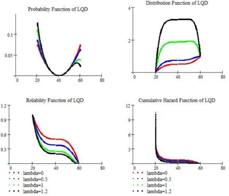
In this paper, transmutation map approach suggested by Shaw and Buckley to define a new model which generalizes the UQ model is used. It is called the generalized distribution as the L-Quadratic Distribution, because the pdf of the LQ distribution takes the form of the small letter "l", as shown in Figure (1). It is denoted by LQ distribution and it is abbreviated LQ(a,b,λ). In the rest of this paper, mathematical formulations with some important related integrations and properties of the LQ distributionare provided, [2].
2.
L- QUADRATIC DISTRIBUTION
According to the Quadratic Rank Transmutation Map (QRTM) approach, the cumulative distribution function (cdf) satisfy the relationship
𝐹 𝑥 = 1 + 𝜆 𝐺 𝑥 − 𝜆𝐺2 𝑥 3
where 𝐺 (𝑥 ) is the cumulative distribution function (cdf) of the base distribution, which on differentiation yields, 𝑓 (𝑥 ) , such that
𝑓 𝑥 = 1 + 𝜆 𝑔 𝑥 − 2 𝜆𝑔 𝑥 𝐺 𝑥 4 If 𝜆 = 0 then the distribution of the base random variable is obtained. By using Eq.(2) and Eq.(3), the cdf of LQ distribution has the following form
𝐹 𝑥 =𝛼3 𝑥 − 𝛽 3 1 −𝛼𝜆 3 𝑥 − 𝛽
3 +1
4 𝜆 + 2 5
where 𝜆 is the transmuted parameter. The corresponding pdf of Eq.(5) is given as follows
𝑓 𝑥 =𝛼 𝑥 − 𝛽 2 1 −2𝛼𝜆 3 𝑥 − 𝛽
3 6 .
3.
STATISTICAL PROPERTIES
Some statistical properties of the new generalization are provided, as follows, [3], [4]:
3.1
Survivor Function
There is a relation between the cdf and the reliability function, i.e., 𝑹𝑭 = 𝟏 − 𝑭(𝒙 ) . Therefore, the Reliability Function (RF) of the LQ distribution (𝑹𝑭𝑳𝑸) is defined as:
𝑅𝐹𝐿𝑄 𝑥 =𝛼3 𝑥 − 𝛽
3 𝛼𝜆 3 𝑥 − 𝛽
3− 1 +1 4 2 − 𝜆
3.2
Hazard Function
There is a relation between the pdf, reliability and hazard function, i.e., 𝒉 𝒙 =𝒇(𝒙)
𝑹(𝒙) Therefore, the Hazard Function
(HF) of the LQ distribution (𝑯𝑭𝑳𝑸) is defined as:
𝐻𝐹𝐿𝑄 𝑥 =
𝛼 𝑥−𝛽 2 1−2𝛼𝜆 3 𝑥−𝛽 3 𝛼
3 𝑥−𝛽 3 𝛼𝜆
3 𝑥−𝛽 3−1 + 1 4 2−𝜆
3.3
Cumulative Hazard Function
There is a relation between the cdf and the cumulative hazard function, i.e., 𝐶𝐻𝐹 𝑥 = − ln 𝐹(𝑥 ). Therefore, the Cumulative Hazard Function (CHF) of the LQ distribution
(𝑪𝑯𝑭𝑳𝑸) is defined as :
𝑪𝑯𝑭𝑳𝑸 𝑥 = −𝑙𝑛 𝛼3 𝑥 − 𝛽
3 1 −𝛼𝜆
3 𝑥 − 𝛽
3 +1
4 𝜆 + 2 .
As shown from Figure (1), the LQ distribution is an extended model to analyze data from complex situations. Also, it is observed that, The pdf and the cumulative hazard function of the LQ distribution takes the form of the small letter "l", but the cdf takes the form of the inverted "∩" quadratic distribution. The LQ distribution has highest reliability at the lower limit "a", and then it is begins decreasing until the median, after that it is increasing again.
3.4
Random Number Generation
To generate random numbers when the parameters a and b are known, the method of inversion can be used from the LQ distribution as
𝑋𝑟𝑣= 𝛽 +
3𝑢 − 0.75 2 + 𝜆 𝛼 − 0.5𝜃 𝑋𝑟𝑣− 𝛽 3
1 3
[image:1.595.54.281.418.503.2]Eq.(7) doesn't have a closed form solution, so “u” will be generated as uniform random variables from U(0,1), and then solve for Xrv in order to generate random numbers from LQ
distribution. From Eq.(7), the quantile Xq of the LQ
distribution is given by 𝑋𝑞 = 𝛽 +
3𝑞 − 0.75 2 + 𝜆 𝛼 − 0.5𝜃 𝑋𝑞− 𝛽 3
1 3
, 𝜃 =2𝛼32𝜆 8
Put 𝑞 = 0.5, the median of the LQ distribution is obtained as 𝑋0.5= 𝛽 +
0.75 𝜆 0.5𝜃 𝑋0.5−𝛽 3−𝛼
1 3
, 𝜃 =2𝛼 2𝜆 3
Also, the percentiles and quartiles can be obtained, by putting different values of 𝑞 in Eq.(8), e.g., the 4th quartiles, 90th percentiles of the LQ distribution is obtained when
𝑞 = 0.25, 𝑞 = 0.90 respectively.
3.5
Useful Important Integrations
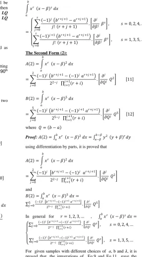
In this paper, the following integrations are developed by two forms for 𝑟 = 1, 2, 3, … as follows:
The First Form (1):
𝐴 1 = 𝑥𝑟 𝑏
𝑎
𝑥 − 𝛽 2 𝑑𝑥
= −1
𝑗 𝑏𝑟+𝑗 +1− 𝑎𝑟+𝑗 +1
𝑗! 𝑟 + 𝑗 + 1
2
𝑗 =0
. 𝜕
𝑗
𝜕𝛽𝑗 𝛽2 9
𝐵 1 = 𝑥𝑟 𝑏
𝑎
𝑥 − 𝛽 5 𝑑𝑥
= −1
𝑗 +1 𝑏𝑟+𝑗 +1− 𝑎𝑟+𝑗 +1
𝑗! 𝑟 + 𝑗 + 1
5
𝑗 =0
. 𝜕
𝑗
𝜕𝛽𝑗 𝛽5 10
Proof
𝐴 1 = 𝑥𝑟 𝑏
𝑎
𝑥 − 𝛽 2 𝑑𝑥 = 𝑥𝑟+2− 2𝛽𝑥𝑟+1+ 𝛽2𝑥𝑟 𝑑𝑥 𝑏
𝑎
= 𝑏
𝑟+3− 𝑎𝑟+3
𝑟 + 3 − 2𝛽
𝑏𝑟+2− 𝑎𝑟+2
𝑟 + 2 + 𝛽
2 𝑏𝑟+1− 𝑎𝑟+1
𝑟 + 1
= −1
𝑗 𝑏𝑟+𝑗 +1− 𝑎𝑟+𝑗 +1
𝑗! 𝑟 + 𝑗 + 1
2
𝑗 =0
. 𝜕
𝑗
𝜕𝛽𝑗 𝛽2
and
𝐵 1 = 𝑥𝑟 𝑏
𝑎
𝑥 − 𝛽 5 𝑑𝑥
= 𝑥𝑟+5− 5𝛽𝑥𝑟+4+ 10𝛽2𝑥𝑟+3− 10𝛽3𝑥𝑟+2+ 5𝛽4𝑥𝑟+1 𝑏
𝑎
− 𝛽5𝑥𝑟 𝑑𝑥
= 𝑏
𝑟+6− 𝑎𝑟+6
𝑟 + 6 − 5𝛽
𝑏𝑟+5− 𝑎𝑟+5
𝑟 + 5 + 10𝛽
2 𝑏
𝑟+4− 𝑎𝑟+4
𝑟 + 4 − 10𝛽3 𝑏𝑟+3− 𝑎𝑟+3
𝑟 + 3 + 5𝛽
4 𝑏𝑟+2− 𝑎𝑟+2
𝑟 + 2 + 𝛽5 𝑏𝑟+1− 𝑎𝑟+1
𝑟 + 1
= −1
𝑗 +1 𝑏𝑟+𝑗 +1− 𝑎𝑟+𝑗 +1
𝑗! 𝑟 + 𝑗 + 1
5
𝑗 =0
. 𝜕
𝑗
𝜕𝛽𝑗 𝛽5
𝑥𝑟 𝑏
𝑎
𝑥 − 𝛽 𝑠 𝑑𝑥
=
−1 𝑗 𝑏𝑟+𝑗 +1− 𝑎𝑟+𝑗 +1
𝑗! 𝑟 + 𝑗 + 1
𝑠
𝑗 =0
. 𝜕
𝑗
𝜕𝛽𝑗 𝛽𝑠 , 𝑠 = 0, 2, 4, …
−1 𝑗 +1 𝑏𝑟+𝑗 +1− 𝑎𝑟+𝑗 +1
𝑗! 𝑟 + 𝑗 + 1
𝑠
𝑗 =0
. 𝜕
𝑗
𝜕𝛽𝑗 𝛽𝑠 , 𝑠 = 1, 3, 5, …
The Second Form (2):
𝐴 2 = 𝑥𝑟 𝑏
𝑎
𝑥 − 𝛽 2 𝑑𝑥
= −1
𝑗 𝑏𝑟+𝑗 +1− −1 𝑗 𝑎𝑟+𝑗 +1
22−𝑗 𝑗 +1 𝑟 + 𝑖 𝑖=1 2
𝑗 =0
. 𝜕
𝑗
𝜕𝑄𝑗 𝑄2 11
𝐵 2 = 𝑥𝑟 𝑏
𝑎
𝑥 − 𝛽 5 𝑑𝑥
= −1
𝑗 𝑏𝑟+𝑗 +1− −1 𝑗 +1 𝑎𝑟+𝑗 +1
25−𝑗 𝑗 +1 𝑟 + 𝑖 𝑖=1 5
𝑗 =0
. 𝜕
𝑗
𝜕𝑄𝑗 𝑄5 12
where 𝑄 = 𝑏 − 𝑎 Proof: 𝐴 2 = 𝑥𝑏 𝑟
𝑎 𝑥 − 𝛽 2 𝑑𝑥 = 𝑦2 𝑏−𝛽
𝑎−𝛽 𝑦 + 𝛽 𝑟𝑑𝑦
using differentiation by parts, it is proved that
𝐴 2 = 𝑥𝑟 𝑏
𝑎
𝑥 − 𝛽 2 𝑑𝑥
= −1
𝑗 𝑏𝑟+𝑗 +1− −1 𝑗 𝑎𝑟+𝑗 +1
22−𝑗 𝑗 +1 𝑟 + 𝑖 𝑖=1 2
𝑗 =0
. 𝜕
𝑗
𝜕𝑄𝑗 𝑄2
and 𝐵 2 = 𝑥𝑏 𝑟
𝑎 𝑥 − 𝛽 5 𝑑𝑥 = −1 𝑗 𝑏𝑟+𝑗 +1− −1 𝑗 +1 𝑎𝑟 +𝑗 +1
25−𝑗 𝑗 +1 𝑟+𝑖 𝑖=1
5
𝑗 =0 .
𝜕𝑗
𝜕𝑄𝑗 𝑄
5
In general for 𝑟 = 1, 2, 3, … , 𝑥𝑏 𝑟
𝑎 𝑥 − 𝛽 𝑠 𝑑𝑥 =
−1
𝑗 𝑏𝑟+𝑗 +1− −1 𝑗 𝑎𝑟+𝑗 +1
2𝑠−𝑗 𝑗 +1 𝑟+𝑖 𝑖=1
𝑠
𝑗 =0 .
𝜕𝑗
𝜕𝑄𝑗 𝑄
𝑠 , 𝑠 = 0, 2, 4, …
−1 𝑗 𝑏𝑟+𝑗 +1− −1 𝑗 +1 𝑎𝑟 +𝑗 +1
2𝑠−𝑗 𝑗 +1 𝑟+𝑖 𝑖=1
𝑠
𝑗 =0 .
𝜕𝑗
𝜕𝑄𝑗 𝑄𝑠 , 𝑠 = 1, 3, 5, …
[image:2.595.264.552.72.593.2]For given samples with different choices of a, b and 𝜆, it is proved that, the integrations of Eq.9 and Eq.11 gave the same results, Table 1 summarizes the results.
Table 1. The Numerical Results of the integrations A(1) and A(2)
𝑛 = 25, 𝑎 = 1.038, 𝑏 = 7.274,
𝜆 = 0.151
𝑛 = 30, 𝑎 = 1.326, 𝑏 = 7.428,
𝜆 = 0.100
A(1) A(2) A(1) A(2)
83.998 83.998 82.889 82.889
Also, for given samples with different choices of a, b and 𝜆, it is proved that, the integrations of Eq.10 and Eq. gave the same results, Table 2 summarizes the results
Table 2. The Numerical Results of the integrations B(1) and B(2)
𝑛 = 25, 𝑎 = 1.038, 𝑏 = 7.274,
𝜆 = 0.151
𝑛 = 30, 𝑎 = 1.326, 𝑏 = 7.428,
𝜆 = 0.100
B(1) B(2) B(1) B(2)
818.725 818.725 703.379 703.379 6805.652 6805.652 6157.646 6157.646 48620.070 48620.070 45522.784 45522.783 338054.080 338054.080 325130.688 325130.684 2340281.552 2340281.552 2305646.766 2305646.738 16210654.402 16210654.402 16342813.696 16342813.506 112473810.571 112473810.571 115981914.625 115981913.316 781800350.335 781800350.335 824421395.565 824421386.519 5443934588.051 5443934588.051 5869711034.899 5869710972.075
3.6
Central Tendency
The mean, median, mode of the LQ distribution can be obtained as follows:
Theorem 1: If 𝑋 a r.v has LQ distribution then the mean is: 𝜇 = 𝜇 1= 𝛽 −
3𝜆
14 𝑏 − 𝑎
Proof: By using the integrations of Eq.9 to Eq.12, the mean of the LQ distribution is:
𝜇 = 𝜇 1= 𝑥 𝑓 𝑥 𝑑𝑥 = 𝑥 𝛼 𝑥 − 𝛽 2−𝜃 𝑥 − 𝛽 5 𝑑𝑥 𝑏
𝑎 𝑏
𝑎
Then, 𝜇 = 𝜇 𝐴
= −1
𝑗 𝑏𝑗 +2− 𝑎𝑗 +2
𝑗! 𝑗 + 2
2
𝑗 =0
. 𝜕
𝑗
𝜕𝛽𝑗 𝛼𝛽2
− −1
𝑗 +1 𝑏𝑗 +2− 𝑎𝑗 +2
𝑗! 𝑗 + 2
5
𝑗 =0
. 𝜕
𝑗
𝜕𝛽𝑗 𝜃𝛽5 13
𝜇 = 𝜇(𝐵)
= 𝛼 −1
𝑗 𝑏𝑗 +2− −1 𝑗𝑎𝑗 +2
22−𝑗 𝑗 +1 1 + 𝑖 𝑖=1 2
𝑗 =0
. 𝜕
𝑗
𝜕𝑄𝑗 𝑄2
− 𝜃 −1
𝑗 𝑏𝑗 +2− −1 𝑗 +1 𝑎𝑗 +2
25−𝑗 𝑗 +1 1 + 𝑖 𝑖=1 5
𝑗 =0
. 𝜕
𝑗
𝜕𝑄𝑗 𝑄5 14
So, 𝜇 = 𝜇 𝐴 = 𝜇 𝐵 = 𝛽 −3𝜆
14 𝑏 − 𝑎 15
[image:3.595.53.273.310.573.2]For different choices of a, b and 𝜆, it is proved that, the forms of the arithmetic mean in Eq.13, Eq.14 and Eq.15 gave the same results, Table 3 summarizes the results.
Table 3. The Numerical Solution of the mean
a b λ 𝜇 𝜇 𝐴 𝜇 𝐵
0.05 0.10 0.50 0.0696 0.0696 0.0696 0.05 0.20 0.75 0.1009 0.1009 0.1009 0.10 1.00 1.00 0.3571 0.3571 0.3571 0.25 1.50 1.50 0.4286 0.4286 0.4286 0.50 1.50 2.00 0.5714 0.5714 0.5714 1.00 2.00 2.50 1.1786 1.1786 1.1786 2.00 3.00 2.75 1.9107 1.9107 1.9107 2.50 3.25 3.00 2.3929 2.3929 2.3929 3.00 4.00 3.50 2.7500 2.7500 2.7500 5.00 10.0 6.00 1.0714 1.0714 1.0714
Theorem 2: If 𝑋 a r.v has LQ distribution then the median is: 𝑚 = 𝛽 + 9𝜆
4𝛼 𝛼𝜆 𝑚 −𝛽 3−3
1 3
Proof:
0.5 = 𝑓 𝑥 𝑑𝑥 = 𝛼 𝑥 − 𝛽 2−𝜃 𝑥 − 𝛽 5 𝑑𝑥
𝑚
𝑎 𝑚
𝑎
=𝛼
3 𝑚 − 𝛽
3 1 −𝛼𝜆
3 𝑚 − 𝛽
3 + 𝜆 + 2
4
Then, 𝑚 = 𝛽 + 4𝛼 𝛼𝜆 𝑚 −𝛽 9𝜆 3−3
1 3
and it is equivalents of Eq.(8).
Theorem 3: If 𝑋 r.v has LQ distribution then the mode is: 𝑚𝑜𝑑𝑒 = 𝑚𝑜 = 𝛽 + 0.6
𝛼𝜆 1 3
Proof: By taking the 1st derivative of Eq.(6) with respect to the r.v X,
𝑓 𝑥 = 2𝛼 𝑥 − 𝛽 3 1 −5𝛼𝜆
3 𝑥 − 𝛽
3
Then, 𝑚𝑜 = 𝛽 + 0.6
𝛼𝜆 1 3
, where 𝑓 𝑥 = 2𝛼 −40 𝛼32 𝜆 𝑥 − 𝛽 3< 0
Theorem 4: If 𝑋 a r.v has LQ distribution then the Harmonic mean (Hm) is:
𝐻𝑚
= 𝛼𝛽2 1 +2𝛼𝜆𝛽3
3 ln 𝑏
𝑎 − 𝛼𝛽 𝑏 − 𝑎
− −1
𝑗 +1 𝑏𝑗 − 𝑎𝑗
𝑗! 𝑗
5
𝑗 =0
. 𝜕
𝑗
𝜕𝛽𝑗 𝜃𝛽5 −1
Proof :
1 𝐻𝑚= 𝐸
1 𝑥 =
1
𝑥 𝑓 𝑥 𝑑𝑥 = 1
𝑥 𝛼 𝑥 − 𝛽
2−
𝑏 𝑎 𝑏
𝑎
𝜃 𝑥 − 𝛽 5 𝑑𝑥 = 𝛼𝛽2 1 +2𝛼𝜆 𝛽
3
3 ln 𝑏
𝑎 − 𝛼𝛽 𝑏 − 𝑎 − −1 𝑗 +1 𝑏𝑗−𝑎𝑗
𝑗 ! 𝑗 5
𝑗 =0 .
𝜕𝑗
𝜕𝛽𝑗 𝜃𝛽
5
Then, 𝐻𝑚 = 𝛼𝛽2 1 +2𝛼𝜆 𝛽3 3 ln
𝑏
𝑎 − 𝛼𝛽 𝑏 − 𝑎 − −1 𝑗 +1 𝑏𝑗−𝑎𝑗
𝑗 ! 𝑗 5
𝑗 =0 .
𝜕𝑗
𝜕𝛽𝑗 𝜃𝛽5
−1
3.7
Moments
Theorem 5: If 𝑋 a r.v has LQ distribution then the rth moments are :
𝜇 𝑟= 𝜇 𝐴𝑟
= −1
𝑗 𝑏𝑟+𝑗 +1− 𝑎𝑟+𝑗 +1
𝑗! 𝑟 + 𝑗 + 1
2
𝑗 =0
. 𝜕
𝑗
𝜕𝛽𝑗 𝛼𝛽2
− −1
𝑗 𝑏𝑟+𝑗 +1− 𝑎𝑟+𝑗 +1
𝑗! 𝑟 + 𝑗 + 1
5
𝑗 =0
. 𝜕
𝑗
𝜕𝛽𝑗 𝜃𝛽5 16
𝜇 𝑟= 𝜇 𝐵𝑟
= 𝛼 −1
𝑗 𝑏𝑟+𝑗 +1− −1 𝑗𝑎𝑟+𝑗 +1
2𝑠−𝑗 𝑗 +1 𝑟 + 𝑖 𝑖=1 2
𝑗 =0
. 𝜕
𝑗
𝜕𝑄𝑗 𝑄𝑠
− 𝜃 −1
𝑗 𝑏𝑟+𝑗 +1− −1 𝑗 +1 𝑎𝑟+𝑗 +1
2𝑠−𝑗 𝑗 +1 𝑟 + 𝑖 𝑖=1 𝑠
𝑗 =0
. 𝜕
𝑗
𝜕𝑄𝑗 𝑄𝑠 17
Proof: Using the integrations of Eq.9 to Eq.12, The rth ordinary moment of the LQ distribution is given by :
𝜇 𝑟= 𝑥𝑟 𝑓 𝑥 𝑑𝑥 = 𝑥𝑟 𝛼 𝑥 − 𝛽 2−𝜃 𝑥 − 𝛽 3 𝑑𝑥 𝑏
𝑎 𝑏
𝑎
Then,
𝜇 𝑟=
−1 𝑗 𝑏𝑟+𝑗 +1−𝑎𝑟+𝑗 +1 𝑗 ! 𝑟+𝑗 +1 2
𝑗 =0 .
𝜕𝑗 𝜕𝛽𝑗 𝛼𝛽
2 − −1 𝑗 +1 𝑏𝑟+𝑗 +1−𝑎𝑟+𝑗 +1 𝑗 ! 𝑟+𝑗 +1 5
𝑗 =0 .
𝜕𝑗 𝜕𝛽𝑗 𝜃𝛽
5 , 𝑟 = 1, 2, …
𝛼 −1 𝑗 𝑏𝑟+𝑗 +1− −1 𝑗𝑎𝑟+𝑗 +1
22−𝑗 𝑗 +1𝑖=1 𝑟+𝑖 2
𝑗 =0 .
𝜕𝑗 𝜕𝑄𝑗 𝑄
2 − 𝜃 −1 𝑗 𝑏𝑟+𝑗 +1− −1 𝑗 +1 𝑎𝑟+𝑗 +1 25−𝑗 𝑗 +1𝑖=1 𝑟+𝑖 5
𝑗 =0 .
𝜕𝑗 𝜕𝑄𝑗 𝑄
5 𝑟 = 1, 2, …
so, 𝜇 1= 𝛽 −
3𝜆
14 𝑏 − 𝑎 , 𝜇 2= 𝑏2+𝑎2
2 −
𝑏−𝑎 2
10 −
3𝜆 𝑏2−𝑎2
14
𝜇 3= 𝑏3+𝑎3
2 −
3 𝑏+𝑎 𝑏−𝑎 2
20 −
𝜆 𝑏3−𝑎3
4 +
3𝜆 𝑏2+𝑎2 𝑏−𝑎
56 −
3𝜆 𝑏−𝑎 3
7 28 , 𝜎2=
3 𝑏−𝑎 2
4 1
5−
3𝜆2
49 .
If 𝜆 = 0 then the first three moments of the base random variable are obtained:
𝜇 1= 𝛽 = 𝜇, 𝜇 2= 𝑏2+𝑎2
2 −
𝑏−𝑎 2
10 , 𝜇 3=
𝑏3+𝑎3
2 −
3 𝑏+𝑎 𝑏−𝑎 2
20 and𝜎
2= 0.15 𝑏 − 𝑎 2
3.8
Moment Generating Function
The moment generating function (mgf) is important especially if it is existing. Then the moment generating function of LQ distribution is derived.
Theorem 6: If 𝑋 a r.v has the LQ distributionthen the mgf is: 𝒎𝒈𝒇𝑳𝑸= 𝑚𝑥 𝑡 =
𝑡𝑟
𝑟!
∞
𝑟=1 𝜇 𝑟
Proof:
𝒎𝒈𝒇𝑳𝑸= 𝑚𝑥 𝑡 = 𝐸 𝑒𝑡𝑥 = 𝑒𝑡𝑥 𝑓 𝑥 𝑑𝑥 = 𝑏
𝑎
𝑒𝑏 𝑡𝑥 𝛼 𝑥 − 𝛽 2−𝜃 𝑥 − 𝛽 3 𝑑𝑥 𝑎
Then
𝒎𝒈𝒇𝑳𝑸= 𝑡
𝑟
𝑟!
∞
𝑟=1 𝑏 𝛼𝑥𝑟 𝑥 − 𝛽 2−𝜃𝑥𝑟 𝑥 − 𝛽 3 𝑑𝑥
𝑎 =
𝑡𝑟
𝑟!
∞
𝑟=1 𝜇 𝑟 15
Put 𝑡 = 𝑖𝑡 in Eq.(15), then characteristic function (QLQ) of the LQ distributionis:
𝑸𝑳𝑸=
𝑖𝑡 𝑟
𝑟!
∞
𝑟=1
𝛼𝑥𝑟 𝑥 − 𝛽 2−𝜃𝑥𝑟 𝑥 − 𝛽 3 𝑑𝑥
𝑏
𝑎
= 𝑖𝑡
𝑟
𝑟!
∞
𝑟=1
𝜇 𝑟
From Eq.(15), notice that, the rth moment is the coefficient of
𝑡𝑟
𝑟! , i.e., 𝜇 𝑟= 𝑐𝑜𝑒𝑓. 𝑜𝑓 𝑡𝑟
𝑟! , and if 𝜆 = 0 then
𝒎𝒈𝒇𝑳𝑸𝑫= 𝑡
𝑟
𝑟!
∞
𝑟=1 𝛼𝑥𝑟 𝑥 − 𝛽 2 𝑑𝑥 𝑏
𝑎 =
𝑡𝑟
𝑟!
∞
𝑟=1 𝜇 𝑟
which is the mgf of the UQ distribution.
4.
PARAMETER ESTIMATION
The maximum likelihood estimates, MLEs, of the parameters that are inherent within the LQ distribution function is given by the following: Let 𝑥1, 𝑥2, … , 𝑥𝑛 be a sample of size n from
LQ distribution, then the likelihood function is given by 𝐿 = 𝛼𝑛 𝑥
𝑖− 𝛽 2 1 −2𝛼𝜆3 𝑥𝑖− 𝛽
3 𝑛
𝑖=1
Put 𝑤𝑖 𝛽 = 𝑥𝑖− 𝛽 and 𝑤𝑖 Φ = 1 −2𝛼𝜆3 𝑤𝑖3 𝛽 , Φ=
𝛼, 𝜆, 𝛽
Then 𝐿 = 𝛼𝑛 𝑤
𝑖2 𝛽 𝑤𝑖 Φ 𝑛
𝑖=1 16
The log-likelihood function of Eq.(16) is given by 𝑙 = ln 𝐿 = 𝑛 ln 𝛼 + 2 ln 𝑤𝑖 𝛽
𝑛
𝑖=1
+ ln 𝑤𝑖 Φ 𝑛
𝑖=1
17
The log-likelihood can be maximized by differentiating Eq.(17) to obtain the maximum likelihood estimate (MLE) of the unknown parameter 𝛼, 𝜆, 𝛽 . Therefore, The 1st
partial derivatives of Eq.(17) with respect to the unknown parameters 𝛼, 𝜆, 𝛽 are given by:
𝜕𝑙 𝜕𝛼=
𝑛 𝛼−
2 𝜆 3 𝑤𝑖
3 𝛽 𝑤 𝑖−1 Φ 𝑛
𝑖=1
𝜕𝑙
𝜕𝛽= 2 𝑤𝑖−1 𝛽 𝛼𝜆 𝑤𝑖3 𝛽 𝑤𝑖−1 Φ − 1 𝑛
𝑖=1
𝜕𝑙 𝜕𝜆= −
2𝛼 3 𝑤𝑖
3 𝛽 𝑤 𝑖−1 Φ 𝑛
𝑖=1
By solving the last three non-linear equations simultaneously, then Φ = 𝛼 , 𝜆 , 𝛽 will be obtained as shown in Section (6).
5.
FISHER’S INFORMATION MATRIX
The 2nd partial derivatives of the 1th partial derivatives of Eq.(17) with respect to the unknown parameters 𝛼, 𝜆, 𝛽 are given as follows:
𝐼1=
𝜕2𝑙
𝜕𝛼2= −
𝑛 𝛼2+
4𝜆2
9 𝑤𝑖6 𝛽 𝑤𝑖−2 Φ 𝑛
𝑖=1
𝐼2=
𝜕2𝑙
𝜕𝛼𝜕𝛽=
2 𝜆
3 𝑤𝑖
2 𝛽 𝑤
𝑖−1 Φ 3 + 2 𝛼𝜆 𝑤𝑖3 𝛽 𝑤𝑖−1 Φ
𝑛
𝑖=1
𝐼3=
𝜕2𝑙
𝜕𝛼𝜕𝜆=
−2
3 𝑤𝑖
3 𝛽 𝑤
𝑖−1 Φ 1 +
2 𝛼𝜆
3 𝑤𝑖
3 𝛽 𝑤
𝑖−1 Φ 𝑛
𝑖=1
𝐼4=
𝜕2𝑙
𝜕𝛽2= −2 𝑤𝑖−2 𝛽 2𝛼𝜆 𝑤𝑖3 𝛽 𝑤𝑖−1 Φ 1 𝑛
𝑖=1
+ 𝛼𝜆𝑤𝑖3 𝛽 𝑤𝑖−1 Φ + 1
𝐼5=
𝜕2𝑙
𝜕𝛽𝜕𝜆= 2𝛼 𝑤𝑖2 𝛽 𝑤𝑖−1 Φ 1 +
2 𝛼𝜆
3 𝑤𝑖3 𝛽 𝑤𝑖−1 Φ
𝑛
𝑖=1
𝐼6=
𝜕2𝑙
𝜕𝜆2= −
4𝛼2
9 𝑤𝑖6 𝛽 𝑤𝑖−2 Φ 𝑛
𝑖=1
𝐼 = −
𝐼1 𝐼2 𝐼3
𝐼2 𝐼4 𝐼5
𝐼3 𝐼5 𝐼6
The approximate 100(1 − 𝛾)% confidence intervals (C.I) for the unknown parameters 𝛼, 𝜆, 𝛽 are given by: B <Φ < 𝐴, 𝑤𝑒𝑟𝑒 𝐴 =Φ + Zγ
2 𝑣𝑎𝑟(Φ ) , 𝐵 =Φ − Z γ
2 𝑣𝑎𝑟(Φ )
6.
APPLICATION OF
LQ
DISTRIBUTION
The estimators and the corresponding summary statistics are obtained by the proposed model using MathCAD program. For a given samples with different choices of a, b and 𝜆 the maximum likelihood estimators (MLEs), the mean squared error (MSE), relative absolute bias (RAB) and the confidence interval are obtained, Table 1, summarizes the results.
Table 4. Estimates the Unknown Parameters with Corresponding Summary Statistics
Initial values MLEs MSE RAB variance Lower limit
Upper Limit n 11 𝛼 0.0492 0.0497 0.4E-6 0.0006 0.0001 0.0496 0.0499 a 1.25 𝛽 4.375 3.9268 0.2009 -0.4482 0.0386 3.8511 4.0025 b 7.5 𝜆 0.15 0.1518 0.3E-5 0.0018 0.0238 0.1052 0.1984 n 20 𝛼 0.0492 0.0495 0.1E-6 0.0003 0.2E-6 0.0494 0.0497 a 1.25 𝛽 4.375 4.1563 0.0479 -0.2188 0.0027 4.1509 4.1616 b 7.5 𝜆 0.15 0.1509 0.9E-6 0.0009 0.0075 0.1362 0.1657 n 25 𝛼 0.0492 0.0495 0.1E-6 0.0003 0.2E-6 0.0493 0.0495 a 1.25 𝛽 4.375 4.1563 0.0479 -0.2188 0.0033 4.1497 4.1628 b 7.5 𝜆 0.15 0.1510 0.1E-5 0.0010 0.0207 0.1105 0.1915 n 30 𝛼 0.0529 0.0528 0.4E-7 -0.6E-4 -0.1E-5 0.0520 0.0529 a 1.3 𝛽 4.35 4.3772 0.0007 0.0272 0.0007 4.3759 4.3785 b 7.4 𝜆 0.1 0.0999 0.2E-7 -0.9E-4 0.0019 0.0962 0.1036
From Table 4, Estimate the true parameters 𝛼, 𝛽, 𝜆 well with relatively small MSEs and RAB. Also it is noticed that, the coverage probabilities of the asymptotic confidence interval are close to the nominal level. These results indicate that the proposed model and the asymptotic approximation work well under the situation. Table 5 summarizes the results of some measures of central tendency and dispersion of the LQ distribution for a given samples with different choices of a, b and 𝜆.
Table 5. Some Measures of Central Tendency and Dispersion of the LQ Distribution
n 11 20 25 30
Mean 3.7243 3.9545 3.9545 4.2466 Median 5.1490 5.1490 5.1490 5.1490
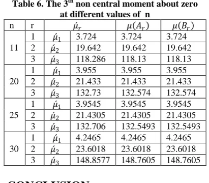
[image:5.595.325.531.202.382.2]Mode 8.2256 8.4718 8.4706 9.2221 Harmonic mean 2.1492 2.4811 2.4815 2.9068 Variance 33.3094 33.5757 33.5556 31.0103 Kurtosis 0.0343 0.0339 0.0339 0.0370 Skewness 0.0112 0.0110 0.0110 0.0077 Pearson1 -0.7799 -0.7796 -0.7796 -0.8935 Pearson2 -2.3398 -2.3388 -2.3389 -2.6805 Also, Table 6 summarizes the results of the 3th non central moment about zero at different values of the sample size distribution.
Table 6. The 3th non central moment about zero
at different values of n
n r 𝜇 𝑟 𝜇 𝐴𝑟 𝜇 𝐵𝑟
11
1 𝜇 1 3.724 3.724 3.724
2 𝜇 2 19.642 19.642 19.642
3 𝜇 3 118.286 118.13 118.13
20
1 𝜇 1 3.955 3.955 3.955
2 𝜇 2 21.433 21.433 21.433
3 𝜇 3 132.73 132.574 132.574
25
1 𝜇 1 3.9545 3.9545 3.9545
2 𝜇 2 21.4305 21.4305 21.4305
3 𝜇 3 132.706 132.5493 132.5493
30
1 𝜇 1 4.2465 4.2465 4.2465
2 𝜇 2 23.6018 23.6018 23.6018
3 𝜇 3 148.8577 148.7605 148.7605
7.
CONCLUSION
Fig. 1. The pdf, cdf, reliability and cumulative hazard functionof LQ distribution
8.
REFERENCES
[1] S.O. Edeki, Hilary Okagbuem and Abiodun Opanuga. 2016. The U-quadratic distribution as a proxy for a transformed triangular distribution (TTD). Research Journal of Applied Sciences, 11 (5): 221-223.
[2] Shaw, W. T., & Buckley, I. R. C. 2007. The alchemy of probability distributions: beyond Gram-Charlier expansions, and a skew-kurtosisnormal distribution from
a rank transmutation map. arXiv preprint arXiv: 0901.0434.
[3] Catherine Forbes, Nicholas Hastings, Brian Peacock and Merran Evans. 2011. Statistical Distributions, 4th ed. A John Wiley & Sons, INC., Publication.
[image:6.595.65.532.75.475.2]