A New Iterative Solution Method for Solving Multiple Linear Systems

A New Iterative Solution Method for Solving Multiple

Linear Systems

Saeed Karimi

Department of Mathematics, Persian Gulf University, Bushehr, Iran Email: [email protected]

Received July 25,2012; revised August 25, 2012; accepted September 8, 2012

ABSTRACT

In this paper, a new iterative solution method is proposed for solving multiple linear systems A x( ) ( )i i =b( )i , for , where the coefficient matrices

1£ £i s A( )i and the right-hand sides are arbitrary in general. The proposed method is based on the global least squares (GL-LSQR) method. A linear operator is defined to con-nect all the linear systems together. To approximate all numerical solutions of the multiple linear systems simultane-ously, the GL-LSQR method is applied for the operato  and the approximate solutions are obtained recursively. The presented method is compared with the well-known LSQR method. Finally, numerical experiments on test matrices are presented to show the efficiency of the new metho

( )i

b

: n s n s

 _´ _´

r

d.

Keywords: Iterative Method; Multiple Linear Systems; LSQR Method; GL-LSQR Method; Projection Method

1. Introduction

We want to solve, using global least squares (GL-LSQR) method, the following linear systems:

( ) ( ) ( ) = , 1 i i i

A x b £ £i s (1)

where A( )i are arbitrary matrices of order n, and in general A( )i ¹A( )j and for In spite of that, in many practical application the coefficient matrices and the right-hand sides are not arbitrary, and often there is information that can be shared among the coefficient matrices and right-hand sides. Multiple linear systems (1) arise in many problems in scientific com- puting and engineering application, including recursive least squares computations [1,2], wave scattering pro- blems [3,4], numerical methods for integral equations [4,5], and image restorations [6].

( )i ( )

b ¹b j

.

i¹ j

Many authors, see [7,8], have researched to approxi- mate the solutions of the multiple linear systems (1) with the same coefficient matrix but different right-hand sides,

i.e.,

( ) ( )

= , 1 . i i

Ax b £ £i s (2) Recently, S. Karimi and F. Toutounian proposed an iterative method for solving the linear systems (2) with the some advantages over the existing methods, see [9- 11], for more details. In [12], Tony F. chan and Michael K. Ng presented the Galerkin projection method for solving linear systems (1). They focused on the seed

projection method which generates a Krylov subspace from a set of direction vectors obtained by solving one of the systems, called the seed system, by the CG method and then projects the residuals of other systems onto the generated Krylov subspace to get the approximate solu- tions. Note that the coefficient matrices in this method are real symmetric positive definite.

In this paper, we propose a new method to solve the linear systems (1) simultaneously, where the coefficient matrices and right-hand sides are arbitrary. We define a linear operator to connect all the linear systems (1) together. Then we apply the GL-LSQR me- thod [13] for the linear operator  and obtain recur- sively the approximate solutions simultaneously. In the new method, the linear operator will be reduced to a lower global bidiagonal, namely -Bidiag, matrix form. We obtain a recurrence formula for generating the se- quence of approximate solutions. Our new method has certain advantages over the existent methods. In the new method, the coefficient matrices

: n s n s

 _´ _´

 

( )i

A and right-hand sides are arbitrary. Also we do not need to store the basis vectors, we do not need to predetermine a subspace dimension and the approximate solutions and residuals are cheaply computed at every stage of the algorithm be- cause they are updated with short-term recurrence.

( )i

b

ple linear systems (1). we also show how to reduce the low-rank approximate solutions to linear operator . The section 4 is devoted to some numerical experiments and comparing the new method with the well known LSQR method, when it is applied to s linear systems independently. Finally, we make some concluding re- marks in section 5.

We use the following notations. For X and Y two ma- trices in n s´ , we consider the following inner product

(

T

)

, _F =

X Y tr X Y , where denotes the trace of a matrix. The associated norm is the Frobenious norm denoted by

( )

.

tr

._F . The notation X ^FY means that

, = 0

X Y _F and X

( )

:,i means that the

i

t column of

X. Finally, we use the notation * for the following product:

h

=1

* = ,

m j j j

y y V



å

(3)

where =

[

1, 2,

]

,

n s m j

V V V V

 _{ Î}´

m for 1 , and

.

j m

£ £

yÎ

By the same way, we define

( )

( )

( )

*T = *T :,1 , *T :, 2 , , *T :,m ,

 é_ë   ù_û (4)

where T is the matrix. It is easy to show that the following relations are satisfied:

m m´

(

)

(

)

(

* y z = *y * , z *T *y= *T

)

,

 +  +   y (5)

where y and z are two vectors of m.

2. The Global Least Squares (GL-LSQR)

Method

In this section, we recall some fundamental properties of GL-LSQR algorithm [13], which is an iterative method for solving the multiple linear systems (2). When all the ’s are available simultaneously, the multiple linear systems (2) can be written as

( )i

b

= ,

AX B (6)

where A is an nonsingular arbitrary matrix, B and

X are an rectangular matrices whose columns are

n n´

s

)

n´

( , ( )1 ( )2

, , s

b b b and x( )1,x( )2,,x( )s , respectively. For solving the matrix Equation (6), the GL-LSQR method uses a procedure, namely Global-Bidiag proce- dure, to reduce A to the global lower bidiagonal form. The Global-Bidiag procedure can be described as follows.

Global-Bidiag (starting matrix B; reduction to global lower bidiagonal form):

1 1 = , 1 1= 1

T

U B V A U

b a

1 1

1 1 1 1

=

, = 1, 2, , =

i i i i i

T

i i i i i

β U AV αU i

α V A U β V

+ +

+ + + +

ü

- _ïï

ýï

- _ïþ 

n s´

(7)

where . The scalars and

are chosen so that , i i

U V Î αi³0 βi³0

= = 1

With the definitions

[

]

[

]

1 2 1 2

1 2 2

1

, , , ,

, , , ,

,

k k

k k

k

k k

k

U U U

V V V

T

 

a

b a

b a

b ₊

º º

é ù

ê ú

ê ú

ê ú

ê ú

º ê ú

ê ú

ê ú

ê ú

ê ú

ë û

 

 

the recurrence relations (7) may be rewritten as:

(

)

1* 1 1 =

k e B,

+ b (8)

1

= *

k k k,

A ₊ T (9)

1 = * 1 1*

T T

k _kk k k k k 1

T .

A  + _ T +a+V+ e+ (10)

For the Global-Bidiag procedure, we have the follow- ing propositions.

Proposition 1 [13]. Suppose that k step of the Global- Bidiag procedure have been taken, then the block

vectors 1 2 and 1 2 are F-

orthonormal basis of the Krylov subspaces

n s´

1

,

k Uk+

T k

, , , _k

V V V U U, ,,U

(

A A V, 1

)



and 1

(

,

T

)

1

k AA U

+ , respectively.

Proposition 2 [13]. The Global-Bidiag procedure will be stopped at step m if and only if , where and l are the grades of V1 and with respect to

{

}

= ,

m min m l

1

U m

T

A A and AAT, respectively.

Proposition 3 [13]. Let k be the matrix defined by

[

1, 2, ,

]

k U U Uk ,

 º 

= 1, ,

i k

where the matrices i , , are generated by the Global-Bidiag procedure. Then

n s´ U

2

* =

k F .

 h h

By using the Global-Bidiag procedure, the GL-LSQR algorithm constructs an approximate solution of the form

= *

k k k

X V y , where y_k = ê_ëéy_k( )1,,y( )_kkù_úûTÎ k, which solves the least-squares problem,

.

min _F

X B-AX

The main steps of the GL-LSQR algorithm can be summarized as follows.

Algorithm 1: Gl-LSQR algorithm

1) Set X0= 0

2) β1= BF, U1=B β1, 1= 1

T F

α A U ,

1= 1

T

V A U α1.

3) Set W1=V1, f1=b1, r1=a1

4) For i= 1, 2, until convergence, Do: 5) W_i = AV_i-α_iU_i

6) βi+1= W_{i F} i F i F

7) Ui+1=Wi βi+1

8) = 1 1

T

i i i i

S A U+ -β+V

9) αi+1= S_{i F}

10) Vi+1=Si αi+1

11) ri=

(

ri2+βi2+1

)

1 2 12) c_i =r r_i

13) si= βi+1 ρi 14) qi+1=si iα+1 15) ri+1=ci iα+1 16) f_i=a_if_i

17) fi+1 =ci if 18) _i= _{i i}

1=

i i

c

f f

i 19) f+ -sf

20) Xi = Xi-1+

(

f ri i

)

Wi 21) Wi+1=Vi+1-

(

qi+1 ri

)

Wi

22) If f_i+₁ is small enough then stop

23) EndDo.

More details about the GL-LSQR algorithm can be found [13].

3. The GL-LSQR-Like Operator Method

In this section, we propose a new method for solving the linear systems (1). For this mean, we define the fol- lowing linear operator

:n s´ n s

 ´

,

(11)

( )

( )1

_{( )}

( )

_{( )}

= :,1 , , s :,

X é_êëA X  A X sù_úû

 (12)

where A( )j , j= 1,,s are the coefficient matrices of the multiple linear systems (1). Therefore, the linear systems (1) is written as:

( )

X =B,

 (13)

where B is an rectangular matrix whose columns are

n s´ ( ) , ( )1 ( )2

, , s

b b b the right hand sides of the linear systems (1).

Definition 1: Let  be linear operator (11). Then

( )

₌ (1)

( )

_{:,1 , ,} ( )

( )

_:,

T _{X A} T_{X A}s T_{X s .}

éêë 

 ùúû

}

,

Consider the block operator (13), similar to the well- known block Krylov subspace

(

)

{

2 1

; = span , , , , m

m A R R AR A R A

-

 R

,

where R is the residual of the operator equation (13), we define the following block Krylov-like subspace.

Definition 2: Let  be linear operator (11). Then

(

)

{

1

( )

}

; = span , ( ), , m

m R R R R

-

   

where = ...

i time i _{  }

    and  is the combination of two operators.

Definition 3: Let  be linear operator (11) and

[

1 2

]

= , , , s

m V V V Î

 n m

m

´

 . Then

( )

=

( ) ( )

1 , 2 , ,

( )

n ms

m V V Vm

´

.

é _{ù Î}

ë  û 

    

where Vj n s,

´

Î j= 1, 2,, .s

To approximate the solution of the block operator Equation (13), we present a new algorithm, will be re- ferred to -GL-LSQR algorithm, which is based on the Global-Bidiag-like procedure, will be referred to - Bidiag. The -Bidig procedure reduces the linear ope- rator to the lower bidiagonal matrix form. This pro- cedure can be described as follows.



 

 -Bidiag (starting matrix B; reduction to lower

bidiagonal matrix form):

( )

1 1= , 1 1= 1

T

βU B αV  U

( )

(

)

1 1

1 1 1 1

=

, = 1, 2, , =

i i i i i

T

i i i i i

β U V αU

i

α V U β V

+ +

+ + + +

üï

-ïý ï

- _ïþ 



 (14)

where _{i i} . The scalars and

are chosen so that

, n s

U V _Î´

0

i

α ³ β_i³0

= = 1

i F i F

Similar to Global-Bidiag procedure, we define

U V .

[

]

[

]

1 2 1 2

1 2 2

1

, , , , , , , ,

.

m m

m m

m

m m

m

U U U

V V V

α

β α

T

β α

β +

º º

é ù

ê ú

ê ú

ê ú

ê ú

º ê ú

ê ú

ê ú

ê ú

ê ú

ë û

 

 

 

According to notation * and by using the definition 3, the recurrence relations (14) may be rewritten as:

(

)

1* 1 1 =

m+ βe B,

 (15)

( )

m = m+1*Tm

   ,

1 T

+

)

(16)

(

1

)

= * 1 1* .

T T

m+ m Tk +am+Vm+ em

   (17)

Proposition 4. Suppose that k step of the -Bidiag procedure have been taken, then the block vectors

1 and 1 are F-orthonormal basis of the Krylov-like subspace and

, respectively.



, , _m

V V

(

T m+

 

1

(

; 1 T

m V

  

, , _m

U U +

)

1 1

The proof of this proposition is similar to that given in [13].

;U



The quantities generated from the linear operator and B by the -Bidiag process will now be used to solve the block least squares problem,

( )

.

min _F

X B X

-

Let the quantities

= * ,

m m m

X  y (18)

(

)

= m

R B- X

m , m

m

(19)

be defined, where m . According to linearity of the operator, it is easy to show that

y Î

(

X_m

)

=

( )

_m *y .

  

Also it readily follows from (15), (16) and properties of product * the equation

( )

(

)

(

)

(

)

1 1 1 1

1 1 1

= *

= * * *

= * ,

m m m

m m m

m m m

R B y

βe T

βe T y

+ + + -     m y

holds to working accuracy.

To minimize the mth residual R_{m F}, since m+1 is F-orthonormal and by using the proposition 3, we choose

so that m

y

1 1 2

=

m F m

R βe -T y_m , (20) is minimum. This minimization problem is carried out by applying the QR decomposition [13], where a unitary matrix Qm is determined so that

[

1 1

]

1

1 1 1

2 3 2

1 1 1 = 0 = , 0 m m m m m

m m m m m m

f

Q T βe

f

r q f

r q f

r q f

r f f + - -+ é ù ê ú ê ú ë û é ê ú ê ú ê ê ê ú ê ú ê ú ê ê ê ú ê ú ë û     ù ú ú ú ú d

where and are scalars. The above factorization is determined by constructing the

m

th plane rotation to operate on rows

m

and

of the transforme

,

l

r q_l f_l

1 + QR , m m Q 1

m+

[

β1 1e

]

to annihilate

1 m

β + . This gives the following simple recurrence re

m T la- tion: 1 1 1

1 m m

m + +

ë ûë û ë û

where 1 0 = , 0 0

m m m

m m m m

m m m

c s

s c β α

r q f

r f

r f

+

+ +

é ù é ù

é ù_ê

ú ê ú

ê ú_ê

ú ê ú

ê_- ú

1 α1

r º , f1ºβ1 and the scalars cm and sm are the nontrivial elements of Qm m, +1 The quantity rm and fm are intermediate sca are subsequently

re d

With setting

,

lars that placed by rm an fm.

1

= *

m m m

y - f



the approximate solution is given by

(

1

= * * ,

m m m m

)

X _{ }- y

(21)

(

1

)

= _m*_m- *f_m. (22) Letting

[

]

1 1 2

* ,

m m m P P Pm

-º º 

  

then

= *

m m m.

X  f

The matrix the last block column of m, can be computed from the previous and , by the simple update

n s´ P_m, 

1 m

P- Vm

(

1

)

= ,

m m m m m

P V -q P- r (23)

also note that,

1

= m ,

m m f f f -é ù ê ú ê ú ë û in which = .

m cm m

f f

Thus, Xm can be updated at each step, via the relation 1

= .

m m m m

X X - +f P

The residual norm R_{m F} is computed directly from the quantity fm+1 as

1

= .

m F m

R f ₊

Some of the work in (23) can be eliminated by using matrices in place of The main steps of the -GL-LSQR algorithm can be summarized as follows.

=

m m m

W r P Pm.



Algorithm 2: -GL-LSQR algorithm

1) Set X0= 0

2) β1= B_F, U1=B β1, 1=

( )

1

T F

α  U ,

( )

1= 1

T

V  U α₁.

3) Set W1=V1, f1=b1, r1=a1

4) For i= 1, 2, until convergence, Do: 5) Wˆ =_i 

( )

V_i -α_iU_i

6) βi+1= Wˆi _F 7) Ui+1=Wˆi βi+1 8) ˆ =

(

1

)

1

T

i i i

S  U+ -β+Vi 9) _{i 1}= ˆ_i

F α+ S

10) Vi+1=Sˆi αi+1 11)

(

2 2

)

1 2

1

= +

i i βi

r r ₊

13) si=βi+1 ρi 14) qi+1=si iα+1 15) ri+1=ci iα+1 16) fi=aifi 17) fi+1 =ci if 18) f_i=c_{i i}f 19) fi+1 =-si if

20) Xi= Xi-1+

(

f ri i

)

Wi 21) Wi+1=Vi+1-

(

qi+1 ri

)

Wi

22) If f_i+₁ is small enough then stop

23) EndDo.

As we observe, the  -GL-LSQR algorithm has certain advantages, we obtain simultaneously the appro- ximate solution of the multiple linear systems (1). Also the residual norm is cheaply computed at every stage of the algorithm.

As a application of the new method applying it to solve the Sylvester equation in a special case. Consider the Sylvester equation

= ,

AX-XB C

where AÎn n´ , CÎn s´ and BÎs s´

=

B Q

are known and is unknown. By using the Schur decom- position for the symmetric matrix B, the above Sylvester equation is returned to the linear systems as follows. There is a unitary matrix Q such that , where is a diagonal matrix which diagonal elements are the eigenvalues of B. So we have

n s´

Î

X

s

T

Q

L

L

ˆ

= = ,

AXQ-XQL CQ C

by taking ˆ =X XQ, the Sylvester equation is converted to the following s linearsystems

( ) ( ) ( )

ˆ j _ˆj _{= ˆ}j_{, = , ,} ,

A x c j i s

where j

( ) ˆ j ₌

,

A A-l I xˆ( )j and cˆ( )j are the j-th col- mun of ˆX and Cˆ, respectively.

4. Numerical Experiments

In this section, all the numerical experiments were com- puted in double precision with some MATLAB codes. For all the examples the initial guess X0 was taken to be zero matrix. We consider two sets of numerical ex- periments. The first set of numerical experiments con- tains matrices of the form

( )

= , = 1, 2, i

i , ,

A A-lI i  s

obtained from the Sylvester equation, explained in previous section, where

10 10

= trdiag 1 , 4, 1

1 1

A

n n

æ _ö÷

ç- + - - ÷

ç _÷

çè + + ø and li is the ei-

genvalue of the matrix

1 = tridiag 1 , 2, 1

1

B

s s

æ _ö÷

ç- + - + ÷

ç _÷

çè + ø

1 1

+ . The right-hand side matrix C is taken where the function

rand creates an random matrix. The matrices of the second set of experiments arise from the three-point

( )

, ,

rand n s

n s´

centered discretization of the operator d

( )

d

d d

u a x

x x

æ _ö÷

ç

- ç_çè ÷_÷ø

in [0,1] where the function a(x) is given by a(x) = c + dx, where c and d are two parameters. The discretization is

performed using a grid size of = 1 65

h , yielding matrices

of size 64 with the values of

and . The right-

hand sides of these systems are generated randomly with their 2-norms being 1. All the tests were stopped as soon as,

(

)

= 0.1551 0.9524 k k

c ´

= 1, 2, ,

k  s

(

)

= 7.7566 0.9524 ,k k

d ´

7 10 .

f _£

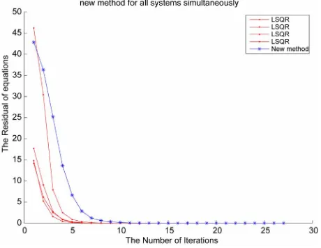
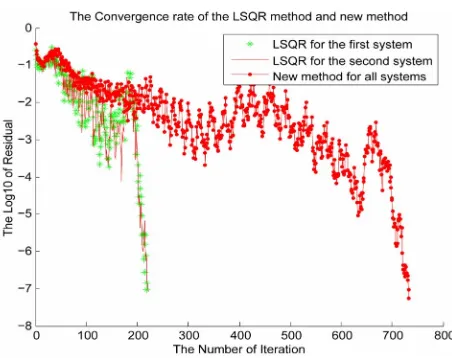
-We display the convergence history in Figure 1 and

Figure 2 for the systems corresponding to the matrices of the first set of matrices and second set of matrices, respectively. Figure 1 shows that the  -GL-LSQR algorithm converges, however, Figure 2 shows slowly convergence which can be remedied by using a reliable preconditioner. But we did not deal with the precon- ditioner techniques in this paper.

5. Conclusion

We proposed a new method for solving multiple linear systems A x( ) ( )i i =b( )i

( )i , for 1 , where the coeffi- cient matrices

i s

£ £

A and the right-hand sides are arbitrary in general. This method has certain advantages which is applied to the arbitrary coefficient matrices

( )i

b

( )i

[image:5.595.309.539.521.699.2]

A and right-hand sides b( )i . Also It is not needed to

[image:6.595.58.284.80.259.2]

Figure 2. Convergence history of the LSQR algorithm and the new algorithm for the second set matrices with s = 2. store the basis vectors, it is not needed to predetermine a subspace dimension and the approximate solutions and residuals are cheaply computed at every stage of the al- gorithm simultaneously because they are updated with short-term recurrence. Applying a reliable preconditioner for the linear systems of Equation (1) may increas the convergence rate, which has not been dicussing in this paper.

6. Acknowledgements

The author would like to thank the anonymous referees for their helpful suggestions, which would greatly in- prove the article.

This work is financially supported by the research com- mittee of Persian Gulf University.

REFERENCES

[1] C. C. Paige and M. A. Saunders, “LSQR: An Algorithm for Sparse Linear Equations and Sparse Least Squares,”

ACM Transactions on Mathematical, Vol. 8, No. 1, 1982, pp. 43-71. doi:10.1145/355984.355989

[2] R. Plemmons, “FFT-Based RLS in Signal Processing,”

Proceeding of the IEEE International Conference on Acous-

tics, Speech and Signal Processing, Minneapolis, 27-30 April 1993, pp. 571-574.

[3] W. E. Boyse and A. A. Seidl, “A Block QMR Method for Computing Multiple Simultaneous Solutions to Compex Symmetric Systems,” SIAM Journal on Scientific Com-

puting, Vol. 17, No. 1, 1996, pp. 263-274.

[4] R. Kress, “Linear Integral Equations,” Springer-Verlag, New York, 1989. doi:10.1007/978-3-642-97146-4

[5] D. O’Leary, “The Block Conjugate Gradient Algorithm and Related Methods,” Linear Algebra and Its Applica-

tions, Vol. 29, 1980, pp. 293-322.

doi:10.1016/0024-3795(80)90247-5

[6] A. Jain, “Fundamentals of Digital Image Processing,” Prentice-Hall, Englewwood Cliffs, 1989.

[7] S. Karimi and F. Toutounian, “The Block Least Squares Method for Solving Nonsymmetric Linear Systems with Multiple Right-Hand Sides,” Applied Mathematics and

Computation, Vol. 177, No. 2, 2006, pp. 852-862.

doi:10.1016/j.amc.2005.11.038

[8] G. Golub and C. Loan, “Matrix Computations,” 2nd Edi- tion, Johns Hopkins Press, Bultimore, 1989.

[9] A. El Guennouni, K. Jbilou and H. Sadok, “The Block Lanczos Method for Linear Systems with Multiple Right- Hand Sides,” Applied Numerical Mathematics, Vol. 51, No. 2-3, 2004, pp. 243-256.

[10] A. El Guennouni, K. Jbilou and H. Sadok, “A Block Bi- CGSTAB Algorithm for Mutiple Linear Systems,” Elec-

tronic Transactions on Numerical Analysis, Vol. 16, 2003, pp. 129-142.

[11] S. Karimi and F. Toutounian, “On the Convergence of the BL-LSQR Algorithm for Solving Matrix Equations,” In-

ternational Journal of Computer Mathematics, Vol. 88, No. 1, 2011, pp. 171-182.

doi:10.1080/00207160903365883

[12] T. F. Chan and M. K. Ng, “Galerkin Projection Methods for Solving Multiple Linear Systems,” SIAM Journal on

Scientific Computing, Vol. 21, No. 3, 2012, pp. 836-850.

doi:10.1137/S1064827598310227

[13] F. Toutounian and S. Karimi, “Global Least Squares (GL- LSQR) Method for Solving General Linear Systems with Several Right-Hand Sides,” Applied Mathematics and

Computation, Vol. 178, No. 2, 2006, pp. 452-460.