Self-Organising Transparent
Learning System
Xiaowei Gu
A thesis presented for the degree of
Doctor of Philosophy
School of Computing and Communications
Lancaster University, England
Supervisor: Prof. Plamen P. Angelov, Ph.D., D.Sc., FIEEE, FIET
Abstract
Machine learning, as a subarea of artificial intelligence, is widely believed to reshape
the human world in the coming decades. This thesis is focused on both the unsupervised and
supervised self-organising transparent machine learning techniques. One particularly
interesting aspect is the transparent self-organising deep learning systems.
Traditional data analysis approaches and most of the machine learning algorithms are
built upon the basis of probability theory and statistics. The solid mathematical foundation of
the probability theory and statistics guarantees the good properties of these learning
algorithms when the amount of data tends to infinity and all the data comes from the same
distribution. However, the prior assumptions of the random nature and same distribution
imposed on the data generation model are often too strong and impractical in real
applications. Moreover, traditional machine learning algorithms also require a number of free
parameters to be predefined. However, without any prior knowledge of the problem, which is
often the case in real situations, the performance of the algorithms can be largely influenced
by the improper choice.
Deep learning-based approaches are currently the state-of-the-art techniques in the fields
of machine learning and computer vision. However, they are also suffering from a number of
deficiencies including the computational burden of training using huge amount of data, lack
of transparency and interpretation, ad hoc decisions about the internal structure, no proven
convergence for the adaptive versions that rely on reinforcement learning, limited
parallelisation and offline training, etc. These shortcomings largely all hinder the wider
applications of the deep learning in real situations.
The novel approaches presented in this thesis are developed within the Empirical Data
Analytics framework, which is an alternative, but more advanced computational methodology
to the traditional approaches based on the ensemble properties and mutual distribution of the
empirical discrete observations.
The novel self-organising transparent machine learning algorithms presented in this
work for clustering, regression, classification and anomaly detection are autonomous,
self-organising, data-driven and free from user- and problem- specific parameters. They do not
impose any data generation models on the data a priori, but are driven by the empirically
problems. In addition, they are highly efficient and suitable for large-scale static/streaming
data processing.
The newly proposed self-organising transparent deep learning systems are able to
achieve human-level performance comparable to or even better than the deep convolutional
neural networks on image classification problems with the merits of being fully transparent,
self-evolving, highly efficient, parallelisable and human-interpretable. More importantly, the
proposed deep learning systems have the ability of starting classification from the very first
image of each class in the same way as humans do.
Numerical examples based on numerous challenging benchmark problems and
comparisons conducted with the state-of-the-art approaches presented in this thesis
demonstrated the validity and effectiveness of the proposed new machine learning algorithms
Statement of Originality
I, Xiaowei Gu, confirm that the work presented in this thesis is my own. Where
information has been derived from other sources, I confirm that this has been indicated in this
Acknowledgements
Firstly, my utmost gratitude goes to my parents for their unconditional supports
throughout the years. Without them, it will not be possible for me to pursue the Ph.D. degree
in UK. I am deeply grateful to my supervisor, Professor Plamen Angelov, for all the very
kind guidance and assistances he provided. The huge amount of time and efforts he spent on
supervising me and the invaluable knowledge and experience he shared with me play the key
role to my research advance. I am pleased to thank Professor Jose Principe and Dr. Dmitry
Kangin for all the discussions and help. Many thanks go to the supervisor in my Master
period in China, Professor Zhijin Zhao for the knowledge, sets of thinking and research skills
she unreservedly passed to me. I also need to express my appreciation to Dr. Shen, Prof.
Table of Contents
Abstract ... i
Statement of Originality ... iii
Acknowledgements ... iv
List of Figures ... ix
List of Tables ... xii
Abbreviations ... xiv
1. Research Overview ... 1
1.1. Motivation ... 1
1.2. Research Contribution ... 3
1.3. Methodology ... 4
1.4. Publication Summary ... 4
1.5. Thesis Outline ... 6
2. Research Background and Theoretical Basis ... 8
2.1. Data Analysis Methodologies Survey ... 8
2.1.1. Probability Theory and Statistics ... 8
2.1.2. Typicality and Eccentricity-based Data Analytics ... 11
2.1.3. Empirical Data Analytics ... 13
2.2. Computational Intelligence Methodologies Survey ... 20
2.2.1 Fuzzy Sets and Systems ... 20
2.2.2. Artificial Neural Networks ... 24
2.2.3. Evolutionary Computation ... 28
2.3. Machine Learning Techniques Survey ... 28
2.3.1. Cluster Algorithms ... 28
2.3.2. Classification Algorithms ... 34
2.3.3. Regression Algorithms ... 42
2.4. Conclusion ... 47
3. Unsupervised Self-Organising Machine Learning Algorithms ... 49
3.1. Autonomous Data-Driven Clustering Algorithm ... 50
3.1.1. Offline ADD Algorithm ... 50
3.1.2. Evolving ADD Algorithm ... 54
3.1.3. Parallel Computing ADD Algorithm ... 59
3.2. Hypercube-Based Data Partitioning Algorithm ... 63
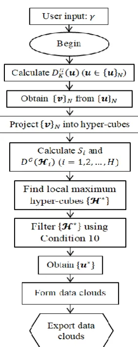
3.2.1. Offline HCDP Algorithm ... 64
3.2.2. Evolving HCDP Algorithm ... 66
3.3. Autonomous Data Partitioning Algorithm ... 69
3.3.1. Offline ADP Algorithm ... 69
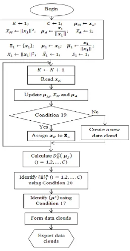
3.3.2. Evolving ADP Algorithm ... 73
3.3.3. Handling the Outliers in ADP ... 75
3.4. Self-Organising Direction-Aware Data Partitioning Algorithm ... 76
3.4.1. Offline SODA Algorithm ... 76
3.4.2. Extension of the Offline SODA Algorithm ... 80
3.4.3. Evolving SODA Algorithm ... 82
3.5. Conclusion ... 85
4. Supervised Self-Organising Machine Learning Algorithms ... 87
4.1. Autonomous Learning Multi-Model Systems ... 87
4.1.1. General Architecture ... 87
4.1.2. Structure Identification ... 88
4.1.3. Parameter Identification ... 91
4.1.4. System Output Generation ... 92
4.2. Zero Order Autonomous Learning Multi-Model Classifier ... 94
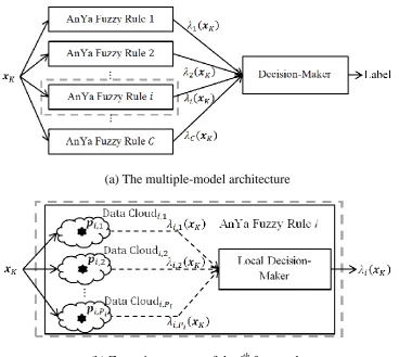
4.2.1. Multiple-Model Architecture ... 94
4.2.3. Validation Process ... 98
4.3. Self-Organising Fuzzy Logic Classifier ... 98
4.3.1. Offline Training ... 99
4.3.2. Online Self-Evolving Training ... 102
4.3.3. Validation Process ... 104
4.4. Autonomous Anomaly Detection ... 105
4.4.1. Identifying Potential Anomalies ... 105
4.4.2. Forming Data Clouds with Anomalies ... 106
4.4.3. Identifying Local Anomalies from Identified Data Clouds ... 107
4.5. Conclusion ... 108
5. Transparent Deep Learning Systems ... 109
5.1. Fast Feedforward Nonparametric Deep Learning Network ... 109
5.1.1. Architecture of FFNDL Network for Feature Extraction ... 110
5.1.2. Architecture of FFNDL Network for Classification ... 114
5.2. Deep Rule-Based Classifier ... 115
5.2.1. General Architecture ... 116
5.2.2. Image Transformation Techniques ... 118
5.2.3. Image Feature Extraction ... 120
5.2.4. Massively Parallel Fuzzy Rule Base ... 122
5.2.5. Decision-Making Mechanism ... 123
5.3. Semi-Supervised DRB Classifier ... 124
5.3.1. Semi-supervised Learning Process from Static Datasets ... 126
5.3.2. Learning New Classes Actively ... 128
5.3.3. Semi-supervised Learning from Data Streams ... 131
5.4. Examples of DRB Ensembles ... 134
5.4.1. DRB Committee for Handwritten Digits Recognition ... 134
5.4.3. DRB Ensemble for Remote Sensing Scenes ... 141
5.5. Conclusion ... 144
6. Implementation and Validation of the Developed Algorithms ... 145
6.1. Evaluation of the Unsupervised Learning Algorithms ... 145
6.1.1. Autonomous Data-Driven Clustering Algorithm ... 148
6.1.2. Hypercube-based Data Partitioning Algorithm ... 153
6.1.3. Autonomous Data Partitioning Algorithm ... 159
6.1.4. Self-Organising Direction-Aware Data Partitioning Algorithm ... 162
6.2. Evaluation of the Supervised Learning Algorithms ... 166
6.2.1. Autonomous Learning Multi-Model System ... 167
6.2.2. Zero Order Autonomous Learning Multi-Model Classifier ... 178
6.2.3. Self-Organising Fuzzy Logic Classifier ... 181
6.2.4. Autonomous Anomaly Detection Algorithm ... 188
6.3. Evaluation of the Transparent Deep Learning Systems ... 193
6.3.1. Fast Feedforward Nonparametric Deep Learning Network ... 193
6.3.2. Deep Rule-Based System ... 198
6.3.3. Semi-Supervised Deep Rule-Based Classifier ... 210
6.4. Conclusion ... 217
7. Conclusion and Future Work ... 218
7.1. Key Contribution ... 218
7.2. Future Work Plans ... 219
List of Figures
Figure 1. Main procedure of the subjective approach for FRB system identification. ... 23
Figure 2. Main procedure of the objective approach for FRB system identification. ... 23
Figure 3. General architecture of a multilayer feedforward NN. ... 25
Figure 4. Example of a decision tree. ... 39
Figure 5. Architecture of the ANFIS. ... 44
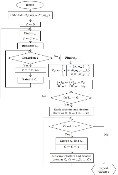
Figure 6. Main procedure of the offline ADD clustering algorithm. ... 54
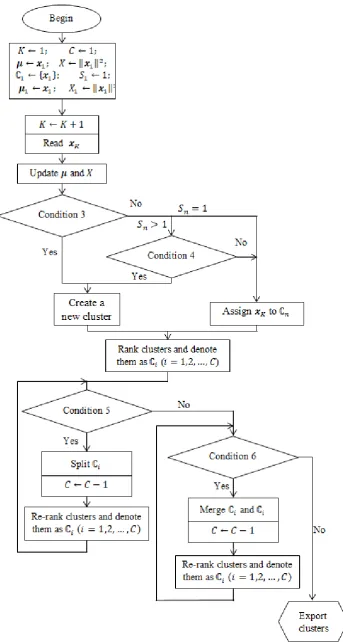
Figure 7. Main procedure of the evolving ADD clustering algorithm. ... 58
Figure 8. Architecture of the parallel computing ADD clustering algorithm. ... 59
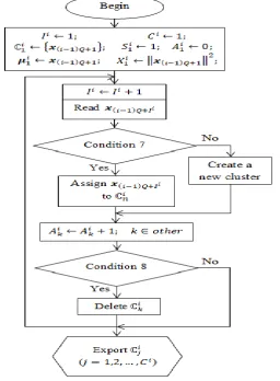
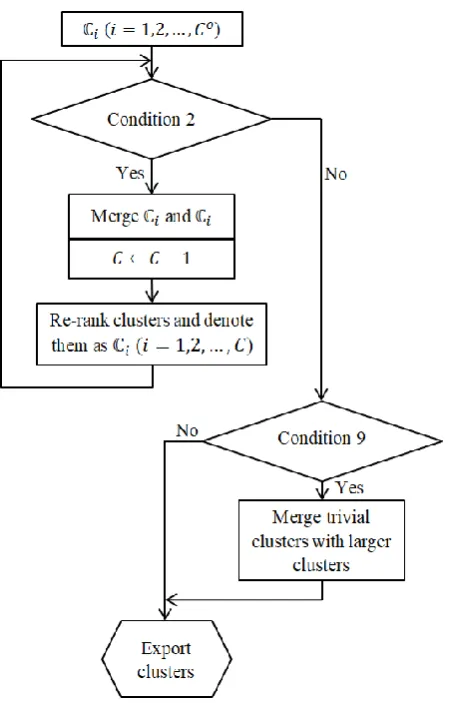
Figure 9. Main procedure of the clustering process of the ith streaming data processor . 62 Figure 10. Main procedure of the fusion process. ... 63
Figure 11. Main procedure of the offline HCDP algorithm. ... 66
Figure 12. Main procedure of the evolving HCDP algorithm. ... 68
Figure 13. Main procedure of the offline ADP algorithm. ... 72
Figure 14. Main procedure of the evolving ADP algorithm. ... 75
Figure 15. Main procedure of the offline SODA algorithm. ... 79
Figure 16. Main procedure of the offline SODA algorithm extension. ... 82
Figure 17. Main procedure of the evolving SODA algorithm. ... 85
Figure 18. Structure of the ALMMO system. ... 88
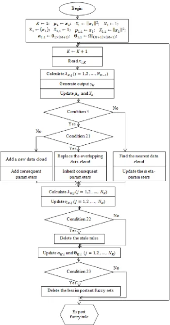
Figure 19. Main procedure of the learning process of the ALMMO system. ... 93
Figure 20. Multiple-model architecture of ALMMO-0. ... 95
Figure 21. Main procedure of the learning process of ALMMO-0 classifier. ... 97
Figure 22. Diagram of the SOFL classifier for offline training. ... 99
Figure 23. Main procedure of the offline training process of SOFL classifier. ... 102
Figure 24. Main procedure of the online training process of SOFL classifier. ... 104
Figure 25. Main procedure of AAD algorithm. ... 108
Figure 26. Architecture of the FFNDL network for feature extraction. ... 110
Figure 27. Architecture of the FFNDL network for classification. ... 114
Figure 28. General architecture of DRB classifier. ... 116
Figure 29. Architecture of the DRB classifier for semi-supervised learning. ... 125
Figure 30. Main procedure of the offline semi-supervised learning of SSDRB classifier. ... 128
Figure 32. Main procedure of the active learning of SSDRB classifier. ... 131
Figure 33. Main procedure of the online semi-supervised learning of SSDRB classifier. ... 133
Figure 34. Architecture of DRB committee for training. ... 135
Figure 35. Architecture of DRB committee for classification. ... 137
Figure 36. Diagram of the cascade of DRB ensemble and SVM. ... 138
Figure 37. Architecture of the DRB ensemble for training. ... 139
Figure 38. Architecture of the DRB ensemble for classification. ... 139
Figure 39. Architecture of the SVM conflict resolution classifier. ... 141
Figure 40. Architecture of the DRB ensemble for remote sensing scenes. ... 142
Figure 41. Structure of the DRB classifier for remote sensing scenes. ... 142
Figure 42. Image segmentation with different sliding windows. ... 143
Figure 43. Clustering results of the ADD algorithm on A2 and S2 datasets. ... 149
Figure 44. Partitioning results of the offline HCDP algorithm with different granularity. ... 155
Figure 45. Partitioning results of the evolving HCDP algorithm with different granularity. ... 156
Figure 46. Partitioning results of the ADP algorithm on Pen-based handwritten digits recognition dataset and Letter recognition dataset... 160
Figure 47. Partitioning results of the SODA algorithm on Wine dataset and Multiple features dataset. ... 163
Figure 48. The evaluation of the extension of the offline SODA algorithm for streaming data. ... 164
Figure 49. Prediction result for the QQSRM problem. ... 168
Figure 50. The evolution of number of data clouds/fuzzy rules. ... 169
Figure 51. Prediction result for the S&P problem. ... 173
Figure 52. Overall classification accuracy on the four benchmark datasets. ... 180
Figure 53. Overall time consumption for training on the four benchmark datasets. ... 181
Figure 54. The average training time consumption with different amounts of training samples. ... 184
Figure 55. The average training time consumption per sample during the online training. ... 185
Figure 56. Visualization of the synthetic Gaussian dataset. ... 189
Figure 58. The identified anomalies by the AAD algorithm. ... 190
Figure 59. The identified anomalies by the ODRW algorithm. ... 191
Figure 60. Example images on human action recognition problem. ... 194
Figure 61. Example images on object classification problem. ... 195
Figure 62. Curves of classification accuracy of the four methods on MNIST dataset. . 196
Figure 63. Examples of images from the database of faces. ... 198
Figure 64. Examples of images from Singapore dataset. ... 199
Figure 65. Example Images from UCMerced dataset. ... 199
Figure 66. Example images of Caltech 101 dataset. ... 200
Figure 67. The relationship curve of training time and recognition accuracy with different amount of training samples. ... 202
Figure 68. Architecture of the DRB classifier for face recognition. ... 203
Figure 69. Architecture of the DRB classifier for object recognition. ... 208
Figure 70. The average accuracy curve of the SSDRB classifier with different values of φ. ... 211
Figure 71. The average accuracy of the SSDRB classifier with different values of L. . 213
Figure 72. Accuracy comparison of the semi-supervised approaches on UCMerced dataset. ... 215
Figure 73. Accuracy comparison of the semi-supervised approaches on Singapore dataset. ... 216
List of Tables
Table 1. A comparison between three types of fuzzy rules ... 22
Table 2. Illustrative example of AnYa fuzzy rules with MNIST dataset ... 123
Table 3. Experimental settings of the comparative algorithms ... 146
Table 4. Details of benchmark datasets for evaluating ADD algorithm ... 148
Table 5. Computational efficiency study under different experimental setting ... 150
Table 6. Performance evaluation and comparison of the ADD algorithm ... 151
Table 7. Performance evaluation and comparison of the ADD algorithm (continue - part 1) ... 152
Table 8. Performance evaluation and comparison of the ADD algorithm (continue - part 2) ... 153
Table 9. Details of benchmark datasets for evaluating HCDP algorithm ... 154
Table 10. Performance evaluation and comparison of the HCDP algorithm ... 157
Table 11. Performance evaluation and comparison of the HCDP algorithm (continue) ... 158
Table 12. Details of benchmark datasets for evaluating ADP algorithm ... 159
Table 13. Performance evaluation and comparison of the ADP algorithm ... 161
Table 14. Performance evaluation and comparison of the ADP algorithm (continue) . 162 Table 15. Details of benchmark datasets for evaluating SODA algorithm ... 163
Table 16. Performance evaluation and comparison of the SODA algorithm ... 165
Table 17. Performance evaluation and comparison of the SODA algorithm (continue) ... 166
Table 18. Example of fuzzy rules identified from the learning progress ... 170
Table 19. Performance demonstration and comparison on QQSRM problem ... 172
Table 20. Performance demonstration and comparison on S&P problem ... 173
Table 21. Overall classification performance-offline scenario ... 175
Table 22. Confusion matrices and the classification accuracy on PIMA dataset ... 176
Table 23. The average true positive rates and true negative rates of the classification results on occupancy detection dataset ... 177
Table 24. Overall classification performance-online scenario ... 177
Table 25. Details of benchmark datasets for evaluating ALMMO-0 classifier ... 178
Table 26. Confusion matrices of classification results on Monk’s problem ... 179
Table 28. Classification performance (in accuracy) with different amount of data for
offline training ... 184
Table 29. Classification performance (in accuracy) with different amount of data for online training following the offline training with 15% of the data ... 185
Table 30. Performance evaluation and comparison for the SOFL classifier ... 187
Table 31. Identified anomalies from the user knowledge modelling dataset ... 192
Table 32. Performance comparison of the anomaly detection algorithms ... 193
Table 33. Recognition results and comparison on MNIST dataset ... 196
Table 34. Time consumption for training process of the FFNDL network ... 196
Table 35. Experimental results of the FFNDL network on image classification ... 197
Table 36. Comparison between the DRB ensembles and the state-of-the-art approaches ... 201
Table 37. Computation time for the learning process per sub-system (in seconds) ... 202
Table 38. Comparison between the DRB classifier and the-state-of-the-art approaches ... 204
Table 39. Visual examples of the AnYa type fuzzy rules ... 205
Table 40. Results with different amount of training samples ... 205
Table 41. Comparison between the DRB classifier and the state-of-the-art approaches on Singapore dataset ... 206
Table 42. Results with different amount of training samples on the Singapore dataset 206 Table 43. Comparison between the DRB classifier and the state-of-the-art approaches on UCMerced dataset ... 207
Table 44. Results with different amount of training samples on the UCMerced dataset ... 208
Table 45. Comparison between the DRB classifier and the state-of-the-art approaches on Caltech 101 dataset ... 209
Table 46. Results with different amount of training samples on the Caltech 101 dataset ... 209
Table 47. Performance of the SSDRB classifier with different values of φ ... 211
Table 48. Performance of the SSDRB classifier with different values of L ... 212
Table 49. Comparison of the semi-supervised approaches on UCMerced dataset ... 214
Table 50. Comparison of the semi-supervised approaches on Singapore dataset ... 216
Table 51. Comparison of the semi-supervised approaches on Caltech 101 dataset ... 217
Abbreviations
AAD − Autonomous Anomaly Detection (Algorithm) ADD − Autonomous Data-Driven (Clustering Algorithm) ADP − Autonomous Data Partitioning (Clustering Algorithm) ALMMO − Autonomous Learning Multi-Model (System) ANFIS − Adaptive-Network-Based Fuzzy Inference System ANN − Artificial Neural Network
APC − Affinity Propagation Clustering ASR − Adaptive Sparse Representation BOVW − Bag of Visual Words
CBDNET − Convolutional Deep Belief Network CDF − Cumulative Distribution Function
CEDS − Clustering of Evolving Data Streams
CLFH − Learning Convolutional Feature Hierarchies CNN − Convolutional Neural Network
CSAE − Convolutional Sparse Autoencoders
DBSCAN − Density-Based Spatial Clustering of Applications with Noise DCNN − Deep Convolutional Neural Network
DDCAR − Data Density Based Clustering with Automated Radii DECNNET − Deconvolutional Networks
DENFIS − Dynamic Evolving Neural-Fuzzy Inference System DLNN − Deep Learning Neural Network
DPC − Density Peaks Clustering (Algorithm) DRB − Deep Rule-Based (System)
DT – Decision Tree
EC – Evolutionary Computation ECM – Evolving Clustering Method EDA − Empirical Data Analytics
EFUNN − Evolving Fuzzy Neural Networks
ELMC − Evolving Local Means Clustering (Algorithm) ETS − Evolving Takagi-Sugeno (Fuzzy System)
FCMMS − Fuzzily Connected Multimodal Systems
FFNDL − Fast Feedforward Nonparametric Deep Learning FRB − Fuzzy Rule-Based (System)
FWRLS − Fuzzily Weighted Recursive Least Squares GGMC − Greedy Gradient Max-Cut (Algorithm) HCDP − Hypercube-Based Data Partition (Algorithm) HOG − Histogram of Oriented Gradients
ID3 − Iterative Dichotomiser 3
IID − Independent and Identically Distributed KDE – Kernel Density Estimation
KNN – K-Nearest Neighbours
LAPSVM – Laplacian Support Vector Machine LCLC – Local-Constraint Linear Coding LGC – Local and Global Consistence LSLR − Least Square Linear Regression LSPM − Linear Spatial Pyramid Matching
MNSIT – Modified National Institute of Standards and Technology MSC – Mean-Shift Clustering
NN – Neural Network
MUFL – Multipath Unsupervised Feature Learning
NMIBC – Nonparametric Mode Identification Based Clustering NMMBC – Nonparametric Mixture Model Based Clustering PDF − Probability Density Function
PMF − Probability Mass Function
QQSRM − QuantQuote Second Resolution Market RBF − Radical Basis Function
RCNET − Random Convolutional Network RDE − Recursive Density Estimation
RLSE – Recursive Linear Least-Square Estimator RS – Random Swap (Algorithm)
RSN − Regularized Shearlet Network
SDAL21M − Sparse Discriminant Analysis via Joint L2,1-norm Minimization
SFC − Sparse Fingerprint Classification
SIFTSC − Scale-Invariant Feature Transform with Sparse Coding SODA − Self-Organised Direction Aware
SOFL − Self-Organising Fuzzy Logic SOM − Self-Organising Map
SPMK − Spatial Pyramid Matching Kernel SSDRB − Semi-Supervised Deep Rule-Based S&P − Standard and Poor
SUBC − Subtractive Clustering SVM − Support Vector Machine
SWLSLR − Sliding Window Least Square Linear Regression TEDA − Typicality-and Eccentricity-Based Data Analytics TLFP − Two-Level Feature Representation
1. Research Overview
This chapter presents the research motivation and summary of the research
contributions, publications and the research methodology. The chapter is organised as
follows. Section 1.1 gives the research motivation. The research contributions are described
in section 1.2. The methodology and publication summary are given in section 1.3 and
section 1.4, respectively. This chapter is finished by the thesis outline.
1.1. Motivation
Nowadays, due to the more matured electronic manufacturing and information
technologies as well as the widely distributed sensors networks, astronomical amount of
streaming data is generated from every area of daily activities. As the world has already
entered the Era of Big Data, data-intensive technologies are now being extensively used by
the developed economies and numerous international organisations. Having realised the
underlying economic benefits in these data, an increasing number of companies, corporations
and research institutions are involved in developing more advanced data analytic and
processing technologies.
Traditional data analytic methodologies [1]–[4] heavily rely on the classical probability
theory and statistics. The appeals of the traditional data analytic methodologies come from
their solid mathematical foundations and their ability that is always guaranteed when the
amount of the data tends to infinity and all the data comes from the same distribution, as
stated by the classical probability theory. Indeed, the traditional probability theory and
statistics [1]–[4] assume the actual data to be realisations of imaginary random variables and
further assume the prior distributions of these variables. However, these appeals also clearly
demonstrate the problems/deficiencies of the traditional methodologies:
1) It is impossible to collect or process the infinity amount of observations;
2) The very strong prior assumptions are often impractical in the real cases;
3)The distribution of the data, or the generation model, is not clear in advance.
These problems/deficiencies more often lead the traditional data analytic approaches to
generate the subjective results, which undermine the effectiveness and correctness of the
Heavily relying on the probability theory and statistics, traditional machine learning
technologies, i.e. clustering, classification, prediction, fault detection, etc., often need users to
predefine various kinds of parameters and prior assumptions in order to guarantee an
effective result [5]–[18]. These predefined parameters and assumptions usually require users
to have a certain extent of prior knowledge and expertise. However, the prior knowledge is
more often unavailable in real cases as the purpose of data analytics is to analyse and
understand the unknown data, not to study the well-understood ones. It is also practically
impossible to empirically predefine parameters for complex problems.
Moreover, most of the existing data processing technologies [5]–[18] were mainly built
upon the basis of the traditional data analytic methodologies [1]–[4]. One cannot expect that
these approaches can get rid of the deficiencies that the traditional probability theory and
statistics suffer from. These data processing technologies often simplify the real data
representation and assume the data following a specific distribution, i.e. the most widely used
Gaussian. The actual data considered in the machine learning literature is usually discrete (or
discretized), which in traditional probability theory and statistics are modelled as a realisation
of the random variable, but one does not know a priori their distribution. If the prior data
generation hypothesis is verified, good results can be expected; otherwise, this opens the door
for many failures.
Besides, many well-known algorithms [5], [6], [13]–[16] as well as some recently
published ones [10] are restricted to offline data processing. Many algorithms also lack the
ability of following the ever-changing data pattern in streaming data. They require a full
retraining when new data patterns emerge.
As the one of so-called latest developments in the fields of machine learning and
artificial intelligence, deep learning [19] is a hot research area attracting the attention of
machine learning researchers as well as the public. Relying on extracting high-level
abstractions in data by using a multiple layer structure composed of linear and non-linear
transformations, the published methods have presented very promising results in image
processing [20]–[24]. Nonetheless, there are three major deficiencies in the current deep
learning methods:
1) The features extracted and the steps to get them by the encoder-decoder methods
2) The training process is off-line and requires a large amount of time as well as
complex computational resources [22]–[24];
3) There are too many ad hoc decisions in terms of structures and parameters [20]–[24].
These deficiencies largely hinder the applications of the deep learning networks in real
problems.
Aiming at overcoming the deficiencies deeply rooted in the traditional probability
theory and statistics, Empirical Data Analytics (EDA) framework is a systematic
methodology of nonparametric quantities recently introduced in [25]–[27] based on the
ensemble properties and mutual distribution of the empirical discrete observations. It touches
the very foundation of data analytics and serves as a strong alternative to the traditional
statistics and probability theory, but is free from the paradoxes and problems that the
traditional approaches are suffering from [26], [27].
The focus of this thesis is the novel machine learning algorithms and deep learning
systems developed within the EDA framework. Compared with traditional ones, these new
approaches presented in this thesis have the following distinctive features:
1) They are self-organising and self-evolving;
2) They are free from prior assumptions and user- and problem- specific parameters;
3) Their structure and operating mechanism are transparent and human interpretable.
These properties of the new approaches presented in this thesis make them appealing
alternatives to both traditional and state-of-the-art methods.
1.2. Research Contribution
This research work focuses on the novel self-organising transparent learning systems.
During the research, the following main contributions have been achieved:
1) Four novel unsupervised machine learning approaches have been developed for
clustering and data partitioning, and they are evaluated on benchmark datasets;
2) Four novel supervised machine learning approaches have been developed for
classification, regressions and anomaly detection problems, and they are evaluated on
3) Two new types of deep learning networks have been proposed for image
classification problems, and they have been applied to various challenging benchmark
datasets from different areas.
1.3. Methodology
This research work is focused on new machine learning algorithms and systems, which
consists of the following parts:
1) Theoretical concepts research;
2) Algorithm implementation;
3) Application and validation.
Based on the theoretical concepts research, the mathematical and analytical description
of the proposed approaches are formulated and investigated, which directly gives an evidence
of the validity and effectiveness of the approaches as well as a basic understanding of their
boundaries and limitations.
Then, the algorithm implementation is to show the practical feasibility of the theoretical
concepts as well as to augment the theoretical analysis.
For the last part, the implemented theoretical concept is tested on benchmark problems
for evaluating its applicability and validity, and it also gives an evidence of the effectiveness
of the algorithms in real situations.
1.4. Publication Summary
The research work presented in this thesis was described in the following publications in
the chronological order by the submission dates:
A. Journal Papers
P. Angelov, X. Gu, D. Kangin, Empirical data analytics, International Journal of
Intelligent Systems, vol. 32(12), pp. 1261-1284, 2017.
P. Angelov, X. Gu, J. Principe, A generalized methodology for data analysis, IEEE
Transactions on Cybernetics, vol. 48(10), pp. 2981 - 2993, 2018.
P. Angelov, X. Gu, J. Principe, Autonomous learning multi-model systems from data
X. Gu, P. Angelov, D. Kangin, J. Principe, A new type of distance metric and its use for
clustering, Evolving Systems, vol. 8 (3), pp.167-177, 2017.
X. Gu, P. Angelov, D. Kangin, J. Principe, Self-organised direction aware data
partitioning algorithm, Information Sciences, vol. 423, pp. 80-95, 2017.
P. Angelov, X. Gu, Empirical Fuzzy Sets, International Journal of Intelligent Systems,
vol.33(2), pp. 362-395, 2018.
X. Gu, P. Angelov, C. Zhang, P. Atkinson, A massively parallel deep rule-based
ensemble classifier for remote sensing scenes, IEEE Geoscience and Remote Sensing
Letters, vol.15(3), pp. 345-349, 2018.
X. Gu, P. Angelov, J. Principe, A method for Autonomous data partitioning,
Information Sciences, vol. 460–461, pp. 65-82, 2018.
P. Angelov, X. Gu, Deep rule-based classifier with human-level performance and
characteristics, Information Sciences, vol. 463-464, pp. 196-213, 2018.
X. Gu, P. Angelov, Semi-supervised deep rule-based approach for image classification,
Applied Soft Computing, vol. 68, pp. 53-68, 2018.
X. Gu, P. Angelov, Self-organising fuzzy logic classifier, Information Sciences, vol.
447, pp. 36-51, 2018
B. Conference Papers
X. Gu, P. Angelov, A. Ali, W. Gruver, G. Gaydadjiev, Online evolving fuzzy rule-based
prediction model for high frequency trading financial data stream, in IEEE Conference
on Evolving and Adaptive Intelligent Systems (EAIS), Natal, Brazil, 2016, pp.169 - 175.
P. Angelov, X. Gu, G. Gutierrez, J. Iglesias, A. Sanchis, Autonomous data density based
clustering method, in International Joint Conference on Neural Networks (IJCNN) ,
Vancouver Canada, 2016, pp.2405-2413.
P. Angelov, X. Gu, D. Kangin, J. Principe, Empirical data analysis: a new tool for data
analytics, in IEEE International Conference on Systems, Man, and Cybernetics (SMC),
Budapest, Hungary 2016, pp. 000052 - 000059.
X Gu, P. Angelov, Autonomous data-driven clustering for live data stream, in IEEE
International Conference on Systems, Man, and Cybernetics (SMC), Budapest,
X. Gu, P. Angelov, G. Gutierrez, J. Iglesias, A. Sanchis, Parallel computing TEDA for
high frequency streaming data clustering, in INNS Conference on Big Data,
Thessaloniki, Greece, 2016, pp.238-253.
P. Angelov, X. Gu, Local modes-based free-shape data partitioning, in IEEE Symposium
Series on Computational Intelligence (SSCI), Athens, Greece, 2016 pp.1-8.
P. Angelov, X. Gu, J. Principe, Fast feedforward non-parametric deep learning network
with automatic feature extraction, in International Joint Conference on Neural Networks
(IJCNN), Anchorage, Alaska, USA, 2017, pp. 534-541.
Angelov, X. Gu, Autonomous learning multi-model classifier of 0-order (ALMMo-0),
in IEEE International Conference on Evolving and Adaptive Intelligent Systems (EAIS),
Ljubljana, Slovenia, 2017, pp. 1-7.
X. Gu, P. Angelov, Autonomous anomaly detection, in IEEE International Conference
on Evolving and Adaptive Intelligent Systems (EAIS), Ljubljana, Slovenia, 2017, pp.
1-8.
P. Angelov, X. Gu, MICE: Multi-layer multi-model images classifier ensemble, in IEEE
International Conference on Cybernetics (CYBCONF), Exeter, UK, 2017, pp. 1-8.
P. Angelov, X. Gu, A Cascade of deep learning fuzzy rule-based image classifier and
SVM, in IEEE International Conference on Systems, Man, and Cybernetics (SMC2017),
Banff, Canada, 2017, pp. 746-751.
1.5. Thesis Outline
The remainder of the thesis is organised as follows.
Chapter 2 - Research Background and Theoretical Basis: contains three parts, the data
analysis methodologies survey, computational intelligence methodologies survey and
machine learning techniques survey. The review serves as the research background and the
theoretical basis of the research works presented in the thesis.
Chapter 3 - Self-Organising Unsupervised Machine Learning Algorithms: proposes
four different unsupervised machine learning algorithms for clustering and data partitioning,
1) autonomous data-driven clustering algorithm [28]–[30]; 2) hypercube-based data
partitioning algorithm; 3) autonomous data partitioning algorithm [31] and 4) self-organising
the EDA computational framework, and thus, are nonparametric, self-organising and entirely
data-driven.
Chapter 4 - Self-Organising Supervised Machine Learning Algorithms: proposes a
first-order autonomous learning multi-model system for regression and classification [34], a
zero-order autonomous learning multi-model classifier [35], a self-organising fuzzy logic
classifier [36] and an autonomous anomaly detection algorithm [37]. These approaches are
also developed within the EDA framework, therefore, they are free from problem- and user-
specific parameters and prior assumptions.
Chapter 5 - Transparent Deep Learning Systems: proposes a fast feedforward
nonparametric deep learning network [38] and deep rule-based systems [39] for image
classification. The semi-supervised, active learning mechanism of the deep rule-based system
is presented [40]. Some successful examples of deep rule-based ensemble classifiers are also
given [41]–[43]. Compared with other deep learning approaches, the deep learning systems
developed within the EDA framework are transparent, nonparametric, feedforward, human
interpretable and free from ad hoc decisions.
Chapter 6 - Implementation and Validation of the Developed Algorithms: presents
numerical examples based on benchmark problems for validating the algorithms presented in
this thesis. A number of state-of-the-art approaches are involved for comparison for a better
evaluation [28]–[43].
Chapter 7 - Conclusion and Future Work: summarises this thesis and gives the
2. Research Background and Theoretical Basis
In this chapter, a review of data analysis methodologies, computational intelligence
methodologies and machine learning techniques is presented serving as the research
background and the theoretical basis of this thesis.
2.1. Data Analysis Methodologies Survey
Data analysis can be described as a process of describing, illustrating and evaluating
data with the goal of discovering useful information, suggesting conclusions, and supporting
decision-making. Besides the engineering, natural sciences and economics, nowadays, other
scientific areas, i.e. biomedical, social science, etc., are also becoming data-centred.
In this section, the traditional data analytics approach (probability theory and statistics)
and the more recently introduced data-centred ones are reviewed.
2.1.1. Probability Theory and Statistics
A key concept in the field of pattern recognition is “uncertainty” [2], [3]. Uncertainty
exists in our daily lives as well as in every discipline in science, engineering, and technology.
Many actions have consequences that are unpredictable in advance just like tossing a coin or
throwing a dice, both of which are simple daily examples. Some of the more complex
examples can be, for example, stock prices changes, foreign currency exchange rates.
Probability theory is about such actions and their consequences. It starts with the idea of an
experiment, being a course of action whose consequence is not predetermined and this
experiment is reformulated as a mathematical object called a probability space [44]. Given
any experiment involving chance, there is a corresponding probability space, and the study of
such spaces is called probability theory [44].
Probability theory provides a consistent framework for the quantification and
manipulation of uncertainties and forms one of the central foundations for pattern recognition
and data analysis [2], [3]. Probability theory serves as the mathematical foundation for
statistics [3] and is essential to many human activities that involve quantitative analysis of
data. The core of the statistical approaches is the definition of a random variable, i.e. a
functional measure from the space of events to the real line, which defines the probability
theory [1]–[4]. Methods of probability theory also apply to study the average behaviour of a
mechanical system, where the state of the system is uncertain, as in the field of statistical
2.1.1.1. Discrete Probability Distribution
Initially, the probability theory considers only the discrete random variables, where the
concept of “discrete” means that the random variables take only finite or countably finite
values in the data space. A probability mass function (PMF) is a function that describes the
probability that a discrete random variable is exactly equal to some value. The PMF is the
primary means of defining a discrete probability distribution, and PMFs exist for random
variables including the multivariate ones in the discrete domains. The formal definition of a
PMF is as [44]:
For a random variable 𝑥 with the value range {𝑥} = {𝑥1, 𝑥2, 𝑥3, … } (finite or countable
infinite), the function,
𝑃𝑥(𝑥𝑘) = P(𝑥 = 𝑥𝑘) for 𝑘 = 1,2,3, …, (2.1)
is called the PMF of 𝑥, where the subscript 𝑥 indicates that this is the PMF of the random variable, 𝑥. As one can see from equation (2.1), PMF is a function that describes the probabilities of the possible values for a random variable and the PMF is defined within a
certain range. In general, there is:
𝑃𝑥(𝑥) = {P(𝑥) 𝑥 ∈ {𝑥}
0 𝑜𝑡ℎ𝑒𝑟𝑤𝑖𝑠𝑒, (2.2)
and PMFs have the following properties [44]:
0 ≤ 𝑃𝑥(𝑥) ≤ 1; (2.3)
∑𝑥∈{𝑥}𝑃𝑥(𝑥)= ∑𝑥∈{𝑥}P(𝑥)= 1; (2.4)
For {𝑥}𝑜 ⊆ {𝑥}, 𝑃𝑥(𝑥 ∈ {𝑥}𝑜) = ∑𝑥∈{𝑥}𝑜P(𝑥). (2.5) The cumulative distribution function (CDF) of the random variable 𝑥, evaluated at 𝑥𝑜, is defined as:
𝐹𝑥(𝑥𝑜) = ∑𝑦∈{𝑥}∧𝑦≤𝑥𝑜P(𝑦). (2.6)
From equation (2.6) one can see that for the discrete random variable 𝑥, the corresponding CDF increases only at the points where it “jumps” to a higher value, and is
constant between these jumps. The points where jumps occur are precisely the values that the
2.1.1.2. Continuous Probability Distribution
Modern probability theory also considers the continuous random variables. A
probability density function (PDF) of a continuous random variable, is a function, whose
value at any given point in its value range can be interpreted as providing a relative likelihood
that the value of the random variable would be equal to that sample, meanwhile, the absolute
likelihood for a continuous random variable to take on any particular value is 0 [44].
In fact, the PDF is used to specify the probability of the random variable falling within a
particular range of values, as opposed to taking on any single value. This probability is given
by the integral of this variable’s PDF over that range.
For a continuous random variable, the probability for it to fall in to the value range of
[𝑥1, 𝑥2] is calculated as [44]:
𝑃𝑥(𝑥1 < 𝑥 < 𝑥2) = ∫ 𝑓𝑥(𝑥)𝑑𝑥 𝑥2
𝑥=𝑥1 , (2.7)
where 𝑓𝑥(𝑥) stands for the PDF of 𝑥. And the CDF of x calculated at 𝑥𝑜 is defined as [44]:
𝐹𝑥(𝑥𝑜) = ∫𝑥𝑜 𝑓𝑥(𝑥)𝑑𝑥
𝑥=−∞ , (2.8)
from which one can see that, the CDF of a continuous random variable is a continuous
function.
PDFs have the following similar properties as the PMFs have:
0 ≤ 𝑓𝑥(𝑥), (2.9)
∫𝑥=−∞+∞ 𝑓𝑥(𝑥)𝑑𝑥= 1. (2.10) One of the commonly used PDFs is the Gaussian function.
2.1.1.3. Problems in Probability Theory and Statistics
Kolmogorov defined the general problem of probability theory as follows [46]:
“Given a CDF, describe outcomes of random experiments for a given theoretical
model.”
Vapnik and Izmailov defined the general problem of statistics as follows [47]:
“Given independent and identically distributed (IID) observations of outcomes of the
Traditional probability theory and statistics have strong and often impractical
requirements and assumptions. They also assume the random nature for the variables [26].
Indeed, the appeal of the traditional statistical approach is its solid mathematical foundation
and the ability to provide guaranteed performance when data is plenty and created from the
same distribution that is hypothesized in the probability law [27]. However, in the field of
machine learning, the actual data considered is usually discrete (or discretised), which in
probability theory and statistics are modelled as the realisations of the random variables.
Moreover, one does not know a priori their distribution. Good results can only be expected on
condition that the prior data generation hypothesis is verified. Otherwise, this opens the door
for failures, namely, meaningless results [27].
Even in the case that the hypothesised measure meets the realisations, one has to address
the difference of working with realisations and random variables, which brings the issue of
choosing estimators of the statistical quantities necessary for data analysis [27]. Moreover,
different estimators may provide different results. The reason is very likely that the functional
properties of the estimators do not preserve all the properties embodied in the statistical
quantities. Therefore, they behave differently in the finite (and even in the infinite) sample
cases [27].
One can conclude that, the major problem of the traditional data analytic approaches is
lying in the strong prior assumptions, which often fail in the reality. As a result, there is a
growing demand for alternative new concepts for data analysis that are centred at the actual
data collected from the real world rather than at theoretical prior assumptions that need to be
confronted for verification with the experimental data as is the case within the traditional
statistical approaches.
2.1.2. Typicality and Eccentricity-based Data Analytics
With this need identified (as stated in the end of the previous section), the so-called
Typicality- and Eccentricity-based Data Analytics (TEDA) approach was introduced in [48]–
[50] as a new concept to address these problems. The core idea of the TEDA approach [48] is
to use the data typicality and eccentricity scores calculated from the data for analysing its
ensemble properties. As it is concluded in [51], TEDA is a data analytics approach to a “per
point” online data analysis without making unrealistic assumptions.
TEDA framework includes the following three operators:
2) Eccentricity;
3) Typicality.
However, TEDA only considers discrete and unimodal operators with the condition that the
operators sum up to 1, not integrate to 1. Development of this concept into a systematic
framework under the name of Empirical Data Analytics (EDA) framework was done in [25]–
[27], and this PhD work was instrumental to this development. In the remainder of this
subsection, the three TEDA operators are summarised. The details of EDA framework will be
presented in the next subsection.
First of all, a real metric space 𝐑𝑀 and a particular data set/stream
{𝒙}𝐾 = {𝒙1, 𝒙2, … , 𝒙𝐾} (𝒙𝑖 = [𝑥𝑖,1, 𝑥𝑖,2, … , 𝑥𝑖,𝑀] 𝑇
∈ 𝐑𝑀) are considered, where 𝐾 > 2; the subscripts denote data samples (for a set) or the time instances when they arrive (for a
stream). In the remainder of this thesis, all the mathematical derivations are conducted in the
𝐾𝑡ℎ time instance by default except when specially declared. The most obvious choice of 𝐑𝑀
is the Euclidean space, but TEDA definitions can be extended to Hilbert space as well.
2.1.2.1. Cumulative Proximity
Cumulative proximity, 𝑞, was firstly introduced in [48]–[50], which can be seen as a square form of farness. It plays an important role in the TEDA framework and is derived
empirically from the observations without making any prior assumptions on the generation
model of the data. The cumulative proximity at 𝒙𝑖, denoted by 𝑞𝐾(𝒙𝑖), is expressed as
(𝑖 = 1,2,3, … , 𝐾):
𝑞𝐾(𝒙𝑖) = ∑𝐾𝑗=1𝑑2(𝒙𝑖, 𝒙𝑗), (2.11) where 𝑑(𝒙𝑖, 𝒙𝑗) denotes the distance/dissimilarity between 𝒙𝑖 and 𝒙𝑗, which can be of any type.
2.1.2.2. Eccentricity
Eccentricity, 𝜉, is defined as the normalised cumulative proximity [48], [49]. It is an important measure of the ensemble property qualifying data samples away from the mode,
and it is useful to disclose distribution tails and anomalies/outliers. The eccentricity at 𝒙𝑖, denoted by 𝜉𝐾(𝒙𝑖), is expressed as (𝑖 = 1,2,3, … , 𝐾):
𝜉𝐾(𝒙𝑖) = 2𝑞𝐾(𝒙𝑖)
∑𝐾𝑗=1𝑞𝐾(𝒙𝑗)
= 2 ∑ 𝑑
2(𝒙 𝑖,𝒙𝑗) 𝐾
𝑗=1
∑ ∑ 𝑑2(𝒙 𝑗,𝒙𝑘) 𝐾
𝑘=1 𝐾 𝑗=1
where the coefficient 2 is used because the distance between 𝒙𝑖 and 𝒙𝑗 is counted twice in the
denominator. From equation (2.12) one can see that 0 ≤ 𝜉𝐾(𝒙𝑖) ≤ 1, and there is
∑𝐾𝑗=1𝜉𝐾(𝒙𝑗)= 2.
Eccentricity can also be normalised as [49]:
𝜁𝐾(𝒙𝑖) = 𝜉𝐾(𝒙𝑖)
2 . (2.13)
Therefore, for the normalised eccentricity, there is ∑𝐾𝑗=1𝜁𝐾(𝒙𝑗)= 1
2.1.2.3. Typicality
Typicality, 𝜏, is defined as a complement of eccentricity (𝑖 = 1,2,3, … , 𝐾):
𝜏𝐾(𝒙𝑖) = 1 − 𝜉𝐾(𝒙𝑖). (2.14) One can tell from the above that the typicality also can be summed up to a constant:
∑𝐾 𝜏𝐾(𝒙𝑖)
𝑗=1 = 𝐾 − 2, (2.15)
and it can be normalised as:
𝑡𝐾(𝒙𝑖) = 𝜏𝐾(𝒙𝑖)
𝐾−2 . (2.16)
Similar to the normalised eccentricity, the sum of the normalised typicality is sum up to
1, ∑𝐾 𝑡𝐾(𝒙𝑖)
𝑗=1 = 1.
The three TEDA operators can be updated recursively online on a sample-by-sample
basis, and the recursive calculation expressions are of paramount in streaming data
processing, the details of which can be found in [48]–[51].
2.1.3. Empirical Data Analytics
The latest development in the field of data analysis, Empirical Data Analytics (EDA)
computational methodology takes the TEDA framework one level further.
As a systematic methodology of nonparametric quantities introduced in [25]–[27] based
on the ensemble properties and mutual distribution of the empirical discrete observations, the
EDA framework is a strong alternative to the traditional statistics and probability theory, but
is free from the paradoxes and problems that the traditional approaches are suffering from
[26], [27]. This is because that all the non-parametric EDA quantities are derived from the
empirically observed data without making any prior assumptions or using predefined
parameters. Thus, it can be viewed as a powerful extension of the traditional probability
EDA framework touches the very foundation of data analytics, and thus, there are a
wide range of applications including, but not limited to, data analysis, clustering, data
partitioning, classification, prediction, anomaly detection, fuzzy rule-based (FRB) system,
deep rule-based (DRB) system, etc.
EDA also serves as the main theoretical basis of the self-organising transparent machine
learning techniques presented in this thesis. In this subsection, the nonparametric discrete
quantities within EDA framework and their corresponding recursive expressions are
summarised. The relationship between EDA quantities and the well-known Chebyshev
inequality [52] is presented as well.
The nonparametric discrete EDA quantities include:
1) Cumulative proximity;
2) Eccentricity and standardised eccentricity;
3) Unimodal and multimodal density;
4) Unimodal and multimodal typicality.
EDA framework shares the same expressions for cumulative proximity and eccentricity
with TEDA, but redefines the typicality in two different versions (unimodal and multimodal),
and further introduces standardised eccentricity, unimodal and multimodal density.
However, it has to be stressed that the EDA framework is not limited to the concepts
presented in this thesis, but to a much wider range in both discrete and continuous domains
[25]–[27].
Firstly, in addition to the TEDA framework presented in section 2.1.2, within the data
set/stream {𝒙}𝐾, it is further taken into consideration that some data samples may repeat more
than once, namely ∃𝒙𝑖 = 𝒙𝑗, 𝑖 ≠ 𝑗. The set of the sorted unique data samples, denoted by
2.1.3.1. Standardised Eccentricity
As the value of eccentricity decreases very fast with the increase of the amount of data,
K (see equation (2.12)), the standardised eccentricity, 𝜀, is introduced as (𝑖 = 1,2,3, … , 𝐾) [48], [49]:
𝜀𝐾(𝒙𝑖) = 𝐾𝜉𝐾(𝒙𝑖) =
2𝑞𝐾(𝒙𝑖) 1
𝐾∑ 𝑞𝐾(𝒙𝑗) 𝐾
𝑗=1
= 2 ∑ 𝑑
2(𝒙 𝑖,𝒙𝑗) 𝐾
𝑗=1 1
𝐾∑ ∑ 𝑑2(𝒙𝑗,𝒙𝑘) 𝐾
𝑘=1 𝐾 𝑗=1
. (2.17)
There is ∑𝐾𝑗=1𝜀𝐾(𝒙𝑗)= 2𝐾.
2.1.3.2. Unimodal density
Unimodal density, D, was firstly introduced in [48] and is redefined as the inverse of
standardised eccentricity in [25], [26]. It plays as the indictor of the main mode within EDA
framework. The unimodal density at 𝒙𝑖, denoted by 𝐷𝐾(𝒙𝑖), is given as (𝑖 = 1,2,3, … , 𝐾):
𝐷𝐾(𝒙𝑖) = 𝜀𝐾−1(𝒙𝑖) =
∑𝐾𝑗=1𝑞𝐾(𝒙𝑗)
2𝐾𝑞𝐾(𝒙𝑖) =
∑𝐾𝑗=1∑𝐾𝑘=1𝑑2(𝒙𝑗,𝒙𝑘)
2𝐾 ∑ 𝑑2(𝒙 𝑖,𝒙𝑗) 𝐾
𝑗=1
, (2.18)
where 0 ≤ 𝐷𝐾(𝒙𝑖) ≤ 1. Unimodal density, in both the discrete and continuous forms, is very fundamental and resembles the membership functions of fuzzy sets, which represents the
degree of truth in fuzzy logic and can take any value from the interval [0,1] [53]. More details of fuzzy sets and systems are given in section 2.2.1. The link between the unimodal
density and membership function is explained in detail in [54].
2.1.3.3. Multimodal density
Multimodal density, 𝐷𝐺 [25]–[27] is valid at the unique data samples only. The multimodal density at the unique data sample 𝒖𝑖 (𝑖 = 1,2,3, … , 𝑁), denoted by 𝐷𝐾𝐺(𝒖𝑖), is defined as the combination of the unimodal density weighted by the corresponding frequency
of occurrence of this unique data sample 𝑓𝑖 as:
𝐷𝐾𝐺(𝒖𝑖) = 𝑓𝑖𝐷𝐾(𝒖𝑖) = 𝑓𝑖
∑𝐾𝑗=1∑𝐾𝑘=1𝑑2(𝒙𝑗,𝒙𝑘)
2𝐾 ∑ 𝑑2(𝒙 𝑖,𝒙𝑗) 𝐾
𝑗=1
. (2.19)
The expression of 𝐷𝐺 is fundamental because it combines information about the
frequencies of occurrence of data samples and their locations in the data space.
2.1.3.4. Unimodal Typicality
In EDA framework, the typicality in the TEDA is redefined and renamed as the
unimodal typicality, which is the normalised data density [25]–[27]. The unimodal typicality
𝜏𝐾(𝒙𝑖) = 𝐷𝐾(𝒙𝑖)
∑𝐾𝑘=1𝐷𝐾(𝒙𝑘)
= ∑ 𝑑
−2(𝒙 𝑖,𝒙𝑗) 𝐾
𝑗=1
∑ ∑ 𝑑−2(𝒙 𝑗,𝒙𝑘) 𝐾
𝑘=1 𝐾 𝑗=1
. (2.20)
The unimodal typicality resembles the traditional unimodal PMF, but is automatically
defined in the data support unlike the PMF which may have nonzero values for infeasible
values of the random variable unless being specifically constrained [27].
2.1.3.5. Multimodal typicality
The multimodal typicality is newly introduced in EDA [25]–[27], which is directly
derived from the experimental data with the ability of providing multimodal distributions
automatically without the need of user decisions or any processing techniques [27]. The
multimodal typicality at a unique data sample 𝒖𝑖 (𝑖 = 1,2,3, … , 𝑁), denoted by 𝜏𝐾𝐺(𝒖𝑖), is expressed as a combination of the normalised unimodal density weighted by the
corresponding frequency of occurrence, 𝑓𝑖:
𝜏𝐾𝐺(𝒖 𝑖) =
𝑓𝑖𝐷𝐾(𝒖𝑖)
∑𝐾𝑘=1 𝑓𝑘𝐷𝐾(𝒖𝑘)
= ∑ 𝑓𝑖𝑑
−2(𝒖 𝑖,𝒖𝑗) 𝐾
𝑗=1
∑𝐾𝑗=1∑𝐾𝑘=1𝑓𝑘𝑑−2(𝒖𝑗,𝒖𝑘)
. (2.21)
The multimodal typicality has the following properties [27]:
1) Sums up to 1;
2) The value is within [0, 1];
3) Provides a closed analytic form;
4) No requirement for prior assumptions as well as any user- or problem- specific
thresholds and parameters;
5) Its value calculated on infeasible data is always zero.
2.1.3.6. Recursive Expressions
The recursive calculation expressions of the nonparametric EDA quantities play a
significant role in streaming data processing. They ensure the processing techniques to be of
one-pass type, and thus, minimise both the memory- and computation- loads.
A. General case
The general recursive expressions of the EDA quantities are given as follows [55]:
𝑞𝐾(𝒙𝑖) = 𝑞𝐾−1(𝒙𝑖) + 𝑑2(𝒙𝑖, 𝒙𝐾); (2.22)
With equations (2.22) and (2.23), all the EDA quantities given in the previous section
can be recursively calculated for all types of distance metric/dissimilarity. If the Euclidean
distance, Mahalanobis distance, cosine dissimilarity or some other types of
distances/dissimilarity are used, one can have more elegant recursive expressions.
B. Euclidean distance case
Using Euclidean distance, defined as 𝑑(𝒙𝑖, 𝒙𝑗) = ‖𝒙𝑖− 𝒙𝑗‖ = √(𝒙𝑖− 𝒙𝑗)𝑇(𝒙𝑖 − 𝒙𝑗), the recursive expression of 𝑞𝐾(𝒙𝑖) and ∑𝐾𝑗=1𝑞𝐾(𝒙𝑗) are given as:
𝑞𝐾(𝒙𝑖) = 𝐾(‖𝒙𝑖 − 𝝁𝐾‖2+ 𝑋𝐾− ‖𝝁𝐾‖2); (2.24)
∑𝐾𝑗=1𝑞𝐾(𝒙𝑗)= 2𝐾2(𝑋𝐾− ‖𝝁𝐾‖2), (2.25)
where 𝝁𝐾 and 𝑋𝐾 are the means of {𝒙}𝐾 and {‖𝒙‖2}𝐾 , respectively, and both of them can
be updated recursively as:
𝝁𝐾 = 𝐾−1
𝐾 𝝁𝐾−1+ 1
𝐾𝒙𝐾; (2.26)
𝑋𝐾 =𝐾−1
𝐾 𝑋𝐾−1+ 1 𝐾‖𝒙𝐾‖
2. (2.27)
C. Mahalanobis distance case
Using Mahalanobis distance [56], defined as 𝑑(𝒙𝑖, 𝒙𝑗) = √(𝒙𝑖 − 𝒙𝑗)𝑇𝚺𝐾−1(𝒙
𝑖− 𝒙𝑗), the
recursive calculation expressions of 𝑞𝐾(𝒙𝑖) and ∑𝐾𝑗=1𝑞𝐾(𝒙𝑗) are given as:
𝑞𝐾(𝒙𝑖) = 𝐾((𝒙𝑖 − 𝝁𝐾)𝑇𝚺𝐾−1(𝒙𝑖− 𝝁𝐾) + 𝑋𝐾− 𝝁𝐾𝑇𝚺𝐾−1𝝁𝐾)
= 𝐾((𝒙𝑖 − 𝝁𝐾)𝑇𝚺
𝐾−1(𝒙𝑖− 𝝁𝐾) + 𝑀) ; (2.28)
∑𝐾𝑗=1𝑞𝐾(𝒙𝑗)= 2𝐾2(𝑋𝐾− 𝝁𝐾𝑇𝚺𝐾−1𝝁𝐾) = 2𝐾2𝑀 ; (2.29)
where 𝝁𝐾 is the mean of {𝒙}𝐾 ; 𝚺𝐾 is the covariance matrix, 𝚺𝐾 = 1
𝐾−1∑ (𝒙𝑘− 𝐾
𝑘=1
𝝁𝐾)(𝒙𝑘− 𝝁𝐾)𝑇; 𝑋𝐾 = 1
𝐾∑ 𝒙𝑘 𝑇𝚺
𝐾 −1𝒙
𝑘 𝐾
𝑘=1 ; 𝑋𝐾− 𝝁𝐾𝑇𝚺𝐾−1𝝁𝐾 = 𝑀[51].
𝚺𝐾 can be updated recursively as:
𝐗𝐾 =𝐾−1
𝐾 𝐗𝐾−1+ 1 𝐾𝒙𝐾𝒙𝐾
𝑇; (2.30)
𝚺𝐾 = 𝐾
𝐾−1(𝐗𝐾 − 𝝁𝐾𝝁𝐾
𝑇). (2.31)
Using cosine dissimilarity, defined as 𝑑(𝒙𝑖, 𝒙𝑗) = √2 − 2𝑐𝑜𝑠 (𝜃𝒙𝑖,𝒙𝑗) = ‖ 𝒙𝑖
‖𝒙𝑖‖−
𝒙𝑗
‖𝒙𝑗‖‖
[32], [33], the recursive calculation expressions of 𝑞𝐾(𝒙𝑖) and ∑𝐾𝑗=1𝑞𝐾(𝒙𝑗) are given as:
𝑞𝐾(𝒙𝑖) = 𝐾 (‖ 𝒙𝑖
‖𝒙𝑖‖− 𝝁̅𝐾‖
2
+ 𝑋̅𝐾− ‖𝝁̅𝐾‖2); (2.32)
∑𝐾𝑗=1𝑞𝐾(𝒙𝑗)= 2𝐾2(𝑋̅𝐾− ‖𝝁̅𝐾‖2), (2.33)
where 𝝁̅𝐾 and 𝑋̅𝐾 are the means of { 𝒙
‖𝒙‖}𝐾 and {‖ 𝒙 ‖𝒙‖‖
2
}
𝐾
, respectively, and both of them
can be updated recursively as:
𝝁 ̅𝐾 =
𝐾−1
𝐾 𝝁̅𝐾−1+ 1 𝐾
𝒙𝐾
‖𝒙𝐾‖; (2.34)
𝑋̅𝐾 = 𝐾−1
𝐾 𝑋̅𝐾−1+ 1 𝐾‖
𝒙𝐾
‖𝒙𝐾‖‖
2
= 1. (2.35)
E. Direction-Aware distance case [33]
The direction-aware distance is a recently introduced distance metric combining the
advantages of Euclidean distance and cosine similarity in the Euclidean space domain. The
direction-aware distance consists of a magnitude component and an angular component and
has the following expression [33]:
𝑑(𝒙𝑖, 𝒙𝑗) = √𝜆𝑀𝑑𝑀2(𝒙𝑖, 𝒙𝑗) + 𝜆𝐴𝑑𝐴2(𝒙𝑖, 𝒙𝑗), (2.36)
where 𝑑𝑀(𝒙𝑖, 𝒙𝑗) = ‖𝒙𝑖 − 𝒙𝑗‖ and 𝑑𝐴(𝒙𝑖, 𝒙𝑗) = √1 − 𝑐𝑜𝑠 (𝜃𝒙𝑖,𝒙𝑗) = 1
√2‖ 𝒙𝑖
‖𝒙𝑖‖−
𝒙𝑗
‖𝒙𝑗‖‖ ; 𝜆𝑀
and 𝜆𝐴 are a pair of scaling coefficients, and there are 𝜆𝑀 > 0 and 𝜆𝐴 > 0.
In [33], the direction-aware distance is proven to be a full metric which satisfies the
following properties for ∀𝒙𝑖, 𝒙𝑗 [57]:
1) Non-negativity: 𝑑(𝒙𝑖, 𝒙𝑗) ≥ 0;
2) Identity of indiscernibles: 𝑑(𝒙𝑖, 𝒙𝑗) = 0 𝑖𝑓𝑓 𝒙𝑖 = 𝒙𝑗; 3) Symmetry: 𝑑(𝒙𝑖, 𝒙𝑗) = 𝑑(𝒙𝑗, 𝒙𝑖);
4) Triangle inequality: 𝑑(𝒙𝑖, 𝒙𝑗) + 𝑑(𝒙𝑖, 𝒙𝑘) ≥ 𝑑(𝒙𝑗, 𝒙𝑘).
With the direction-aware distance, the recursive calculation expressions of 𝑞𝐾(𝒙𝑖) and
𝑞𝐾(𝒙𝑖) = 𝐾 ((‖𝒙𝑖 − 𝝁𝐾‖2+ 𝑋𝐾− ‖𝝁𝐾‖2) + 1 2(‖
𝒙𝑖
‖𝒙𝑖‖− 𝝁̅𝐾‖
2
+ 1 − ‖𝝁̅𝐾‖2)); (2.37)
∑𝐾𝑗=1𝑞𝐾(𝒙𝑗)= 𝐾2(2(𝑋𝐾− ‖𝝁𝐾‖2) + 1 − ‖𝝁̅𝐾‖2), (2.38)
where 𝝁𝐾, 𝑋𝐾 and 𝝁̅𝐾 can be updated recursively using equations (2.26), (2.27) and (2.34). 2.1.3.7. Chebyshev Inequality
The well-known Chebyshev inequality in the traditional probability theory and statistics
[52] describes the probability that a certain data sample 𝒙, is more than 𝑛𝜎 distance away from the mean, 𝝁, where 𝜎 denotes the standard deviation. With the Euclidean distance used, the Chebyshev inequality can be reformulated as [2]–[4]:
𝑃(‖𝒙 − 𝝁‖2 < 𝑛2𝜎2) > 1 − 1
𝑛2, (2.39)
and the possibility of the point 𝒙 to be an outlier is given by:
𝑃(‖𝒙 − 𝝁‖2 ≥ 𝑛2𝜎2) ≤ 1
𝑛2. (2.40)
It can be proven that exactly the same result can be provided within EDA through the
standardised eccentricity for the Euclidean distance [49]:
𝑃(𝜀𝐾(𝒙𝑖) < 1 + 𝑛2) > 1 − 1
𝑛2; (2.41)
𝑃(𝜀𝐾(𝒙𝑖) ≥ 1 + 𝑛2) ≤ 1
𝑛2. (2.42)
Similarly, the Chebyshev inequality in the form of density is expressed as [26]:
𝑃 (𝐷𝐾(𝒙𝑖) > 1
1+𝑛2) > 1 −
1
𝑛2 ; (2.43)
𝑃 (𝐷𝐾(𝒙𝑖) ≤ 1 1+𝑛2) ≤
1
𝑛2. (2.44)
One can see that the attractiveness of equations (2.41)-(2.44) in comparison with
equations (2.39)-(2.40) is that no prior assumptions are required within EDA on the nature of
the data (random or deterministic), the generation model, the amount of data and their
independence. In addition, the results are more elegant and similar expressions can be derived
for Mahalanobis distance, cosine dissimilarity as well as other types of distance and
![Figure 5, where two fuzzy rules of Takagi-Sugeno type are considered [59], [62]:](https://thumb-us.123doks.com/thumbv2/123dok_us/9329072.434874/61.595.75.477.179.450/figure-fuzzy-rules-takagi-sugeno-type-considered.webp)