ASH Search: Binary Search Optimization
Ashar Mehmood
School of Electrical Engineering and Computer Science (SEECS) National University of Science and Technology (NUST)
Islamabad, 44000, Pakistan
ABSTRACT
The binary search is a method of finding the position of an element in an ordered array. It continuously aims the middle element of array and check if it is the target element or not untills it finds its position. The best case complexity of binary search is O(1), whereas average and worst case time complexity is O(log n), where ‘n’ is the number of elements in the array. In this paper, I have proposed an algorithm which drastically improves the complexity of search algorithm in sorted array domain outperforming binary search, the paper also compares the proposed solution with other well-known search algorithms. The presented approach minimizes the space complexity, eliminates the need to analyze the scenario and look for the algorithm that best fits the given problem. The proposed algorithm has constant space complexity (O(1)) and time complexity of O(1) (constant time) in best case, O(log(log n)) in average case and O(log(n)) in worst case. Thus, most of the time proposed algorithm works very well as compared to other search algorithms in sorted array domain.
General Terms
Theory of computation, Design and analysis of algorithms, Data structures design and analysis, Sorting and searching
Keywords
Binary search, Sorted searching, Search optimization, Interpolation search, complexity analysis.
1.
INTRODUCTION
Search aim to retrieve object or information with specified features and constraints in large search space or bulk of data. An object or information can be value or set of values, assign to a variable, satisfy a specific constraint. Searching works on sorted list of elements and unsorted list of elements as well. As a proper database is used to fix in the large amount of data, searching often used algorithms that query the data structure to extract required information. Often, search algorithms depend on the data structure being searched. On the basis of data structure being used for the data storage, a suitable search algorithm is chosen. Sometimes, it has some prior knowledge about the type of data being searched. Both aforementioned factors help the algorithm to extract the specific information efficiently.
Applications of search algorithms are everywhere. Everyone who uses smartphone or computer is directly or indirectly taking advantages of search algorithms such as finding a word in any text editor, searching any song in playlist or searching contact number by name, number in cell phone etc. In online shopping websites we search for the products. Similarly there are many applications of search algorithms. Any search operations you come across involve search algorithms. There are various types of algorithms used to search an element from bulk of elements. They usually return a success or a failure status, usually denoted by Boolean true/false. Different types of search algorithms are used for different
purposes and their performance and efficiency depend on the data and on the mechanism in which they are used. All search algorithms can be classified based on their searching mechanism but normally they are classified as traditional search algorithm and proposed search algorithm.
Traditional search algorithms are those which are used very frequently or in normal day life or in our academia e.g linear search[1], Binary or half-interval search[1], Digital search[2], hashing[1], interpolation search[3], jump search[4] etc. However, searches outside a linear search require sorted data. Proposed search algorithms are those which are proposed by researcher’s recently e.g network localization using tree search algorithm [5], Quadratic search [6] etc.
The algorithm presented in this paper is related to traditional search algorithms. Thus, we will not discuss about proposed algorithms and all the comparison of presented algorithm in this paper is with some of traditional search algorithms. Presented algorithm works on sorted data, similar to binary search; it proceeds using an element of data as its basis, predicting whether or not it is the target element in a given iteration. However, unlike binary search which repeatedly targets the middle element of the search structure and divides the search space in halves with each iteration, the proposed solution accounts for the nature of data given, similar to interpolation search (mentioned below), which can be an instrumental factor in optimizing the search efficiency. Like Interpolation search [3], presented algorithm considers the type of data and caters variations between the elements of data, in search space, being searched. It estimates the position of targeted value. After comparison, it divides the search space according to the estimate index and discard that search space which is not useful anymore, in finding that value (confirmed that value is not in that part of search space).Inshort, unlike binary search, which divides the search space into half, the presented approach reduces the search space to the part before or after the estimated postion or index. The algorithm repeatedly does the same steps until the target value is found.
2.
RELATED WORKS
Uniform binary search[1] is another search algorithm invented by Donald Knuth. It stores the index of middle element instead of lower and upper bounds. It also stores the change in the middle element between two consective iterations (current and next iteration). But this method is faster in those cases only where it is inefficient to calculate middle point, e.g decimal computer [7].
search takes atmost log2x, where x is the position of target value. Exponential search is an improvement over binary search only in that case when target value lies near the beginning of the array.
Fractional cascading [9] is another search technique introduced by Chazelle and Guibas in 1986. It divides the sorted searching array into multiple sorted arrays and searches each array separately. Searching each array separately needs O(k log n) times (k is the number of arrays: result of original array fragmentation) but fractional cascading searches any element in O(k+log n) times because it stores some specific information about each elements and its position of each array in other arrays. Thus, it needs some extra space to compute the index.It is used in solving computational geometry problem [10] efficiently and data mining [11] as well. Interpolation search [3] is another search algorithm firstly described by W. W. Peterson in 1957. Like proposed algorithm it estimates the index of target element and in the next iteration, remaining search space reduced to the part before or after the estimated index. There is an estimation formula to estimate the index of target element. Interpolation search has average time complexity of O(log(log(n))) which is better than binary search but in worst case(e.g when elements increase exponentialy) its estimation is very inaccurate and it can take O(n) iterations.
Quadratic search [6] is another search algorithm recently introduced by Parveen Kumar in March, 2013. It was an improvement over binary search. Instead of targeting the middle element it targets the middle,1/4th and 3/4th element of sorted array and check whether one of these elements is searched/target element or not. If one of these element is the target element then it immediately returns that element otherwise it reduce the search space after checking many cases. It has worst case complexity of O(log(n/2)). No doubt that it works very well as compared to binary search but its biggest disadvantage is that it is very costly (a lot of condition is to be checked for the reduction of search space and index calculation). When an array is searched containing millions number of elements then quadratic search has to perform many index calculations and condition checking which is not good. Moreover, in average case too it will take log(n/2) steps which is not better than log(log n) and the presented approach is very less costly as compared to quadratic approach. Similarly, there are many other search algorithms for different purposes e.g Quantum binary search [12], Noisy binary search [13][14], Fibonacci search [15]. Each has their own advantages and disadvantages.
The proposed algorithm estimates the target element index using a formula nearly same as one used in interpolation search. Moreover, it doesn’t collapse in anycase e.g elements increase exponentialy or very different variation of variations between the elements of array. Similar to binary search, it takes log(n) in worst case whereas interpolation search takes O(n) in worst case. For instance of average case it takes log(log(n)) like interpolation search. Thus, the proposed approach is better than interpolation and binary search as well. The main comparison in this paper is amongst presented, binary and interpolation search algorithm.
3.
ALGORITHM
Ash_search(arr<vector>,s_num,t_elem) est_var0;
est_indx0;
start0; endt_elem-1; while(start<=end)
est_var (arr[end]-arr[start])/(end-start); est_n ((s_num-arr[start])/est_var)+start; if(arr[est_n]==s_num)
return est_n; else
if(s_num>arr[est_n]) startest_n+1; else
endest_n-1;
if(arr[start+((0.5)*(end-start))]<=s_num) startstart+((0.5)*(end-start));
else
endend-((0.5)*(end-start)); return -1;
3.1
Description
In proposed algorithm,arr<vector>: Dynamic array containing all the elements. s_num: target element.
t_elem: total number of elements in arr<vector>
est_var: average variation computed between the elements of data.
est_n: estimated index of target element on the basis of estimated variation between the elements of data.
start: starting index of instantanious array. end: ending index of instantanious array.
3.2
Logical point of view
The algorithm runs within the starting and ending index of the array.
The algorithm finds the average variation between elements of array so that it can find with how much average variation elements are coming.
As target element lie between starting and ending index of the array so algorithm estimates the position of target number by just dividing it by the average variation.
Due to large variation of variations between the elements of array, average variation can be inaccurate (don’t fulfill between all the elemets of the array). Thus, in this case estimated index would be very inaccurate and algoritm has to update the array starting and ending index so that in the next iteration the estimation can be more accurate.
Moreover, the array is reduced to half to get more accurate estimated variation and estimated index in the next iteration.
3.3
Algorithmic point of view
Presented algorithm works on a single loop. Each iteration does the following set of operations:
Calculating average variation between the elements of array.
Calculating estimated index of target element on the basis of calculated average variation between the elements of array.
Checking whether the element on the estimated index is equal to target element or not.
If the element on the estimated index is not equal to target element then update the starting and ending index of the array to converge to target element.
If target element is greater than element on the estimated index then it means that the target element lies between the estimated index and ending index. Thus, now our starting index will be estimated_index+1.
If target element is smaller than element on the estimated index then it means that the target element lies between the starting index and estimated index. Thus, now our ending index would be estimated_index-1.
Discard the 50% part of instantanios array from the right or left side such that the target element remains in the updated array and estimations can be more accurate.Consider the case where there is a vector containing 30 elements coming with different variations in ascending order arr= {21, 27, 35, 58, 59, 60, 67, 69, 85, 95, 120, 151, 152, 157, 160, 166, 174, 181, 192, 197, 204, 209, 219, 225, 229, 235, 241, 248, 251, 263}
For example, we want to find the position of of element “67”, where subtraction of elements (arr[end]-arr[start]), subtraction of indexes (end-start) and difference of starting index element from target element (s_num-arr[start]) is represented by △ (Delta), Ω (Omega), µ (mu) respectively.
In first iteration: Start0 endt_elem-1
est_var8.34483△⁄Ω est_n6 (µ⁄(est_var))+start;
After comparing the element at 6th index with target element it is noted that they are equal. Thus, in this case proposed algorithm finds the elements in first iteration.
Now, suppose we want to find 192, In first iteration:
start0 endt_elem-1
est_var8.34483△⁄Ω est_n20(µ⁄(est_var))+start;
As, at 20th index element is 204, which is greater than 192 so proposed algorithm changes the starting and ending index to make estimation more accurate and find correct index of element 192. Thus,
start9start+((0.5)*Ω) end19 est_n-1; In second iteration: est_var10.2△⁄Ω
est_n19 (µ⁄(est_var))+start;
As, at 19th index element is 197, which is still greater than 192 so proposed algorithm again changes the starting and ending index. Thus,
start13start+((0.5)*Ω) end18 est_n-1; In third iteration: est_var7△⁄Ω
est_n18 (µ⁄(est_var))+start;
At 18th index the element is 192 which is equal to target element. Thus, proposed algorithm finds the target element in 3 iterations.
With the help of average variation and index estimation formula, we ended up with estimated index of target element. We can noticed that after comparing the estimated index element with target element in second iteration the starting and ending index is updated.There are two types of updation is performed in the proposed algorithm: first on the basis of estimated index and second is just cutting the array from left or right side. The purpose of both the updation is to converge to the target element quickly.
On the basis of estimated index:
s_num>arr[est_n]: If target element is greater than element at the estimated index then it is obvious that to acquire more accurate estimation of target element we have to start from next index of current estimated index. Therefore, “start” becomes “est_n+1” (As arr[est_n]!=s_num, so there is no need to consider est_n in new array).
s_num<arr[est_n]: If target element is smaller than element at the estimated index then it is obvious that to acquire more accurate estimation of target element we have to update our ending index. As we know that the target element is smaller than estimated index so it would be better to consider “est_n-1” as ending index in next iteration. Thus, it will give better estimation in next iteration.
Suppose there is an array whose elements comes with very
different variations such as,
arr={16,81,256,625,1296,2401,4096,6561,10000,14641,1464 2,14643,14644,20736,83521,104976}. It can be noticed that difference between first two element of array is 65 and difference between next two elements is 175. Similarly, difference between 3rd and 4th element is 369 and so on. But difference between 10th and 11th element is just 1 and same is the case for 11th, 12th and 12th, 13th. It can also be noticed that the variation in the last four elements are 6092, 62785, 21455.Thus, with this much variation in the variations between the elements of array the average variation estimation would not be better enough to give accurate result for the estimate index. Here comes the second part of updation of starting and ending index.
4.
EXISTING APPROACHES
Usually binary search and linear search considered as best search algorithms for sorted and unsorted arrays respectively. Binary search does not consider the type of data (whether elements in the data structure increase linearly, exponentialy or with different variations) in the data structure but considering it can be helpful in more efficient searching. There are two other search techniques which are little bit better than binary search for some cases, Interpolation search[3] and hash table[1].
Similar to presented algorithm interpolation search estimates the position or index of target element and reduced the search space to the part before or after the estimated index. Same steps is taken untill it finds the target element. Interpolation search works well when the elements of data is distributed equally but it collapse when elements increase exponentially or increase with very different variations.
In “search using hash value” approach we insert the elements into a hash implemented data structure e.g Hashtable or HashMap[1]. As in this approach elements of hashmap indexed by a specific code e.g hashcode, the time to search any element of data structure would almost take constant time (O(1)). But the huge disadvantage of this approach comes out when the number of elements are large. In this case, it leads collision and it requires more space for the elements. Thus, it is difficult to use when number of elements is large.
5.
PROPOSED APPROACH
The presented algorithm does not collapse in any case. It is not affected by the type of data e.g data is increasing exponentially or data is increasing with very different variations. In average, it takes fewer iteration as compared to binary search to search an element in a data structure and it has no space overhead (does not use any extra array other than searching array). In even worst case, it takes iterations more or less equal to binary search. Thus, the presented algorithm is the best choice to search an element in sorted data structure.
6.
EXPERIMENTAL ANALYSIS
Table 1. Author’s laptop specifications
Dell Inspiron 15 3542
Processor Intel Pentium 3558U Core Dual Core Processor 1.7GHz, Core i3
Storage 1 TB, 5400 rpm
System memory 4GB DDR3-1600 Graphic card (integrated) Intel HD Graphics 4400
The efficiency of search algorithm is measured by number of times the comparison is made with target element. We can say that the number of iteration a target element takes to be searched in a data structure under worst case circumstances decides the algorithm’s efficiency. To test the proposed approach against best algorithms so far and to show little bit comparison between algorithms, some tests are designed. The specification and result of different tests are as follow: TS = Total number of searches which have been made in a test.
LI = Number of searches in which an algorithm takes less iterations than binary search.
MI = Number of searches in which an algorithm takes more iterations than binary search.
EI = Number of searches in which an algorithm takes equal iterations to binary search.
TI = Total iterations an algorithm takes to make all the searches.
MaxI = Maximum number of iterations an algorithm takes to make any search in a test.
AvgI = Average number of iterations an algorithm takes to make all the searches in a set of test.
Algo. = Algorithms.
Interp. = Interpolation search. Bin. = Binary search. Pre. = Presented algorithm
[image:4.595.308.550.325.398.2]In every test each element is searched.Considering the array containing 501 nearly equally distributed elements array={2,3,5,8,9,11,14,15,17,20,21,23,26,…..,1001 }. The results of different algorithms are as follow:
Table 2.0. Equally distributed elements
Algo. TS LI MI EI TI MaxI AvgI
Interp. 501 498 1 2 834 2 1
Bin. 501 - - - 4007 9 7
Pres. 501 500 0 1 501 1 1
As the data were equally distributed so estimating the index of target element was easy. That’s why in this case interpolation algorithm works well as compared to binary search and proposed algorithm is even better than interpolation search. The point to be noted here is that number of iterations is a vague criterion for measuring the efficiency of an algorithm because of the reason that there can be many operations in an iteration of an algorithm than other algorithm’s iteration. Thus, we are comparing the efficiency of the presented approach with existing solutions in terms of number of operations as well. Comparison, addition, subtraction, division etc are considered an operation. Operational analysis of above test is given below:
LO: Number of searches in which an algorithm takes less operation than binary search.
MO: Number of searches in which an algorithm takes more operation than binary search.
EO: Number of searches in which an algorithm takes equal operation to binary search.
TO: Total operations an algorithm takes to make all the searches in a set of test.
MaxO: Maximum number of operations an algorithm takes to make any search in a set of test.
Table 2.1. Equally distributed elements(Operational Analysis)
Algo. LO MO EO TO MaxO AvgO
Interp. 491 7 3 7005 17 13
Bin. - - - 17800 43 35
Pres. 500 1 0 3507 7 7
It can be noticed that the result obtained by operational analysis is not much different than the previous approach (comparison on the basis of iteration).
Now consider the array containing 1000 elements increasing randomly whereas the random function for this test is given as:
Next_element=Previous_element+ (random() * 1000 +1) It means that random number is from 1 to 1000 and every next element is the addition of previous element and generated random number. The results of different algorithms are as follow:
Table 3.0. Random generated elements
Algo. TS LI MI EI TI MaxI AvgI
Interp. 1000 991 4 5 2754 7 2
Bin. 1000 - - - 8987 10 8
Pres. 1000 994 4 2 2613 5 2
Table 3.1. Random generated elements(Operational Analysis)
Algo. LO MO EO TO MaxO AvgO
Interp. 934 58 8 22217 53 22
Bin. - - - 39991 48 39
Pres. 940 52 8 22714 47 22
It can be noticed that average number of iterations and operations that binary takes to search an element is very large as compared to interpolation and presented algorithm. This is because of not considering the type of data. Both interpolation and presented approach consider the variations between the data. Thus, they converge to target element with very less iterations and operations. However, in this case too presented algorithm has minimum MaxI and MaxO.
Now consider the case where interpolation fails to produce efficient result. It is the case when there is equally distributed data but at the end there are few elements which have a very large variation from its previous element e.g outlier elements or there are some equally distributed data and there are some data coming with very different variation e.g cluster of elements. For example, in this test we assumed an extreme situation of aforementioned case represented as array = {1, 2, 3, 4, 5, 6, …….. , 997, 998, 999, 1000000999}. The results of different algorithms are as follow:
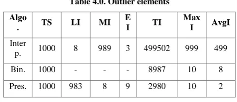
Table 4.0. Outlier elements
Algo
. TS LI MI E
I TI
Max I AvgI
Inter
p. 1000 8 989 3 499502 999 499
Bin. 1000 - - - 8987 10 8
Pres. 1000 983 8 9 2980 10 2
Table 4.1. Outlier elements(Operational Analysis)
Algo. LO MO EO TO MaxO AvgO
Interp. 5 995 0 4494511 8990 4494
Bin. - - - 39991 48 39
Pres. 795 192 13 28782 110 28
The reason for interpolation search failure in efficient searching in this case is the large variation between 999th and 1000th elements. When there are some elements which have great difference in variation between them, as compared to variations between other elements, then average variation becomes biased towards large variation (average variation comes out very larger and gives estimated index very far from actual index) which affects the searching of other elements(e.g all the elements excepts outliers). On the other hand, presented algorithm does not fail in this case because it reduces the search space into half from one of either side, which is suitable for next estimation and due to reduction of search space, estimation becomes more accurate. This is why most of the time presented approach converges to the searched element in fewer numbers of operations. When we look closely towards the efficiency of different algorithms in operational analysis, it can also be noticed that the MaxO of presented algorithm is greater than that of binary search; it does not matter much because most of the time presented approach works very well as compared to binary search (from AvgO) and the case where there is only one outlier with this much variation from previous elements is very rare. The result gets better when we consider real life situations which usually don’t have just one outlier but some outliers or clusters of elements.
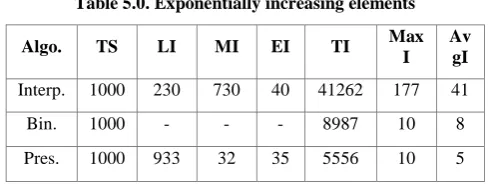
Now consider the case where elements increase exponentially. This is the case where each pair of elements has variation vary with large amount than other pair of elements’ variation.As a result the average variation comes out is very disturbed which cause very wrong prediction of index of target element.Thus, interpolation search fails to perform efficient searching in this case too. However, presented algorithm works very well as compared to interpolation in this case too because it shortens the search space with each iteration to give better average variation which helps in better prediction of index of target element. Exponential function for this test is given below: Next_element=i*i*i*i
[image:5.595.49.285.97.169.2]Table 5.0. Exponentially increasing elements
Algo. TS LI MI EI TI Max I
Av gI
Interp. 1000 230 730 40 41262 177 41
Bin. 1000 - - - 8987 10 8
[image:6.595.44.290.76.168.2]Pres. 1000 933 32 35 5556 10 5
Table 5.1. Exponentially increasing elements (Operational Analysis)
Algo. LO MO EO TO MaxO AvgO
Interp. 118 880 2 370358 1592 370
Bin. - - - 48978 60 50
Pres. 330 648 22 54506 109 54
When elements increase exponentially, variation between the elements of data/array also increases and as a result, the average variation becomes biased towards large variation. Due to biased average variation (toward large variation between the elements at the end part of array), the index estimation is very wrong for the elements near the beginning of array. Interpolation search takes several numbers of iterations to find the target element becaurse after predicting a very wrong index it moves forward in linear fashion e.g suppose it predicts 2nd index but actual index is 28 then in next iteration it predicts 3rd index and in next interation it predicts 4th index and so on (same is the situation for set of test “Outliers elements”). However, the presented algorithm works well in this case because it reduces the search space with each iteration. Due to which better average variation comes out and prediction of target element’s index is more accurate. But in operational analysis of set of test 3 and 4, it can also be noticed that in case of the maximum number of operations “MaxO” taken by the presented algorithm exceeds the maximum number of operations binary search takes, which depicts that the efficiency of presented approach is slightly lower as compared to binary when elements have very different variations. However, it does not have a significant effect in even these cases, most of the time, presented algorithm takes less operations than binary search as we can see in the “AvgO” column of the operational analysis and these cases are rare too.
Moreover, there are some more test has been run on the presented algorithms. In these test too, presented approach works better as compared to other search algorithms. One of these tests includes string searching. For this test, a CMUdict[16] (Carnegie Mellon University) Pronouncing Dictionary (an open-source machine-readable pronunciation dictionary for North American English that contains over 134,000 words and their pronunciations) is used. To perform this test, a hashing function is used to convert each string/word into a unique number according to their characters (in that word/string). Each word/string is searched in this test, about 132905 searches have been made, out of which in 132524 searches, presented algorithm works better than binary search, in 178 searches it works the same as binary search and in rest of the searches presented algorithm takes a few more iterations than binary search. It was noticed that the presented approach takes maximum of log n steps in searching any word/string (17 iterations max.) and in average
it takes log (log n) steps (only 4 or 5 iterations), which is a huge advantage over other search algorithms.
7.
COMPLEXITY ANALYSIS AND ITS
COMPARISON
In best case, all the three algorithms have constant time complexity. As presented algorithm estimate the position of target element on the basis of estimate variation between the elements of array. Suppose, if the elements of array increase with equal variation or has equally distributed data. Then, average variation comes out will be very accurate. Therefore, presented algorithm finds the target element in constant time.
For example, an
array={2,4,5,8,9,11,12,14,16,18,20,22,23,25,27} contained equally distributed data. All the searches made to this array will be in constant time. Thus, the time complexity of presented algorithm in best case is O(1).
In average case, the performance of presented algorithm is slight better as compared to interpolation search and way better than binary search because in average case presented algorithm estimates the position of target element on the basis of average variation which is not so disturbed because elements are coming with random variations. Thus, it converges to target element taking very less iteration as compared to binary search. As, we are using the same approach as interpolation search so we can say that the average case complexity of presented algorithm is same as interpolation search O(log(log(n)) where ‘n’ is the number of elements in the data structure/array . It can be noticed that the reduction of search space in presented algorithm follows both the techniques e.g search space reduction technique used in interpolation and binary search. But in average case, reduction is biased towards one used in interpolation search(even in first iteration average variation is accurate enough to move very close to target element due to which reduction using binary search technique is not so needed ). If we talk about binary search, it is not affected by any variation or other factors. It does not concerend with how elements of data are increasing. It just targets the middle element and discards half of the elements. Thus, its time complexity in average case is O(log n).
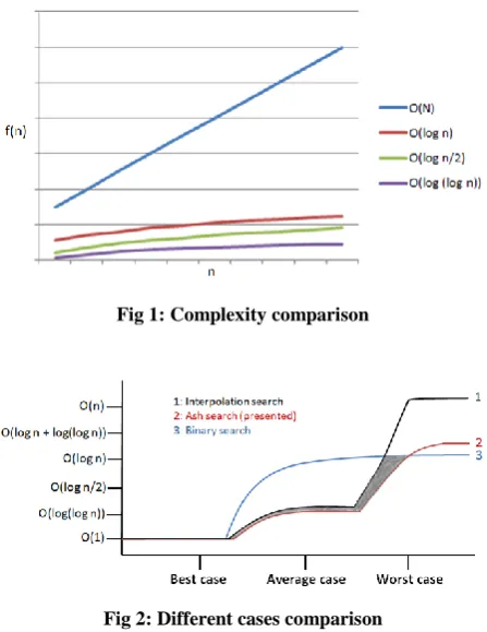
Fig 1: Complexity comparison
Fig 2: Different cases comparison
In Figure 2, it can be noticed that the presented algorithm is a drastic improvement over binary and interpolation search. In worst case, interpolation search totally fails to produce result efficiently but presented algorithm works well. The main advantage of presented algorithm is in average and some of the worst case scenarios. The grey shaded region represents the cases where the proposed approach works more efficiently as compared to both interpolation and binary search. These cases include randomly increasing elements, clusters of elements, outliers etc in search space. In rest of the cases, presented approach works more or less the same as binary search. Thus, it is better to use proposed approach than other algorithm in any case.
8.
ADVANTAGES AND
DISADVANTAGES
Presented algorithm can be used in any scenario and eliminates the need of analyzing the given problem to look for the apt algorithm. Presented algorithm works well in all scenarios and has better efficiency than all the best search algorithms in sorted array domain. Less iteration is needed to find the target element, no need of extra space and execution time is also better than other algorithms. There is as such no cons of presented approach other than that it is slight more costly (calculation of estimation formula and search space reduction calculation makes it more costly). However, even after including these extra costs to the algorithm’s time complexity, it works very well in best and average cases but works almost identical to binary search in worst case. Another disadvantage is that it only works on numbers (If you find a string in a batches of string, you will have to convert array of string into array of numbers using some hashing function)
9.
CONCLUSION
The algorithm introduced in this paper has done a great improvement over existing search algorithms in sorted data domain. It covers all the different aspects of existing search algorithms where these algorithms have defficieny in more
efficient searching. This is why, in average case, the result is computed using fewer iterations as compared to the best available approaches. Moreover, as presented algorithm covers all the possibilites of data variation, it can be used in any scanerio without analyzing it. All other algorithms have their own disadvantages. Some fails to perform efficient searching in worst case, some doesn’t consider the type of data and some uses extra resources. While presented algorithm has constant space complexity and worst case time complexity of O (log n), its real advantage is in average case and some of worst case scenario when it performs searching within O (log (log n)) steps. In sorted data searching, the presented approach will be the best option. Further, it can also be expanded to other applications of search algorithms.
10.
ACKNOWLEDGMENT
The author thanks Dr. Muhammad Ali Tahir (Assistant professor, Department of Computing-SEECS) for his guidance and inspiration.
11.
REFERENCES
[1] D. E. Knuth, “The Art of Computer Programming”, Vol. 3: Sorting and Searching, Addison Wesley, 1973. [2] F. Plavec, Z. G. Vranesic, Stephen D. Brown, “On
Digital Search Trees: A Simple Method for Constructing Balanced Binary Trees”, in Proceedings of the 2 nd
International Conference on Software and Data Technologies (ICSOFT ’07), Vol. 1, Barelona, Spain, July 2007, pp. 61-68.
[3] W. W. Peterson, “Addressing for Random-Access Storage”, IBM Journal of Research & Development, doi: 10.1147/rd.12.0130, 1957.
[4] Ben Shneiderman, “Jump Searching: A Fast Sequential Search Technique”, Communications of the ACM, Vol. 21, NY, USA, Octuber 1978, pp. 831-834, doi: 10.1145/359619.359623.
[5] Phisan Kaewprapha, Thaewa Tansarn, Nattankan Puttarak, “Network localization using tree search algorithm: A heuristic search via graph properties”, 13 th International Conference on Electrical Engineering/Electronics, Computer, Telecommunications and Information Technology (ECTI-CON), 2016. [6] Parveen Kumar, “Quadratic Search: A New and Fast
Searching Algorithm (An extension of classical Binary search strategy)”, International Journal of Computer Applications, Vol. 65, Hamirpur Himachal Pradesh, India, March 2013.
[7] Hermann Von Schmid, “Decimal Computation (1 st ed)”, John Wiley & Sons Ins., NY, USA, 1974.
[8] J. L. Bentley, A. C. Yao, “An almost optimal algorithm for unbounded searching”, Vol. 5, Issue 3, Information Processing Letters, pp. 82-87, doi: 10.1016/0020-0190(76)90071-5, ISSN 0020-0190, 1976.
[9] B. Chazelle, L. J. Guibas, “Fractional cascading: A data structuring technique”, Algorithmica, Vol. 1, Issue 1-4, pp. 133-162, November 1986.
[11]Jaiwei Han, Micheline Kamber, Jian Pei, “Data Mining: Concepts and Techniques (3 rd ed.)”, ISBN: 978-0-12-381479-1, June 2011.
[12]Vladimir Korepin, Ying Xu, “Binary Quantum Search”, International Journal of Modern Physics B, Vol. 21, ISSN 5187-5205, doi: 10.1117/12.717282, May 2007. [13]Andrzej Pelc, “Searching with known error probability”,
Theoretical Computer Science, pp. 1855-2022, doi: 10.1016/0304-3975(89)90077-7, 1989.
[14]R. L. Rivest, A. R. Meyer, D. J. Kleitman, “Coping with errors in binary search procedures”, STOC ’78
Proceedings of the 10 th annual ACM symposium on Theory of computing, doi: 10.1145/800133.804351, pp. 227-232, San Diego, California, USA, 1978.
[15] David E. Ferguson, “Fibonaccian searching”, Communications of ACM, Vol. 3, Issue 12, NY, USA, doi: 10.1145/367487.367496, 1960.