Minimizing Complementary Pivots in a Simplex-Based
Solution Method for a Quadratic Programming Problem
Elias Munapo
Department of Decisions Sciences, University of South Africa, Pretoria, South Africa Email: [email protected]
Received July 12, 2012; revised August 14, 2012; accepted August 29,2012
ABSTRACT
The paper presents an approach for avoiding and minimizing the complementary pivots in a simplex based solution method for a quadratic programming problem. The linearization of the problem is slightly changed so that the simplex or interior point methods can solve with full speed. This is a big advantage as a complementary pivot algorithm will take roughly eight times as longer time to solve a quadratic program than the full speed simplex-method solving a linear problem of the same size. The strategy of the approach is in the assumption that the solution of the quadratic program-ming problem is near the feasible point closest to the stationary point assuprogram-ming no constraints.
Keywords: Quadratic Programming; Convex; Karusha-Kuhn-Tucker; Simplex Method
1. Introduction
The quadratic programming (QP) problem is the problem of optimizing a quadratic function over a convex solution space. A variety of methods are available for solving the quadratic programming problem [1-6]. These include interior point, extensions of the simplex, gradient project- tion, conjugate gradient, augmented Lagrangian and ac- tive set methods.
Simplex-method: The simplex-method was proposed by George Dantzig in 1947 and it searches the boundary of the feasible solution for the optimal solution [7]. The main problem with this method is that it has an exponent tial complexity and is affected by degeneracy and cycling. This method has undergone so many improvements and has been competitive for solving practical linear pro- gramming (LP) problems so far.
Interior point method: This is a method that reaches the optimal solution of a linear programming model by traversing the interior of the feasible region contrary to simplex method [3,8,9]. The interior point approaches were mainly developed for the general nonlinear pro- gramming problem but were later abandoned because of their poor performance that time. Karmarkar’s break- through in 1984 revitalized the study of interior point methods which have been shown to have a polynomial complexity. The interior point algorithm has competed well with the simplex-method on large LPs. The other four methods are not as competitive as these two for LPs. Detailed information on the other methods will not be presented here but readers are encouraged to see Freund [3] or Sun and Yuan [10] for more information.
Application of quadratic programming: Quadratic programming has been successfully applied in areas such as engineering, finance, economics, agriculture, market- ing, public policy, water resource management and trans- portation. The following are some of the so many spe-cific applications of quadratic programming.
Monopolist’s profit maximization Portifolio selection
Inequality constrained least-squares estimation Goal programming with quadratic preferences
Spatial equilibrium analysis for optimal allocation and pricing
Optimal linear decision rules
Calculation of current flow in resistors Optimization of digital filters
Image classification in Computer Vision
Numerical modeling of elastoplastic contact problems Optimization of chemical process synthesis
More on applications of quadratic programming can be found in Gupta [11], Horst et al. [12] and McCarl et al.
method solving a linear problem of the same size [4]. The strategy of the approach is in the assumption that the solution of the quadratic programming problem is near the feasible point closest to the stationary point assuming no constraints.
2. The Quadratic Programming Problem
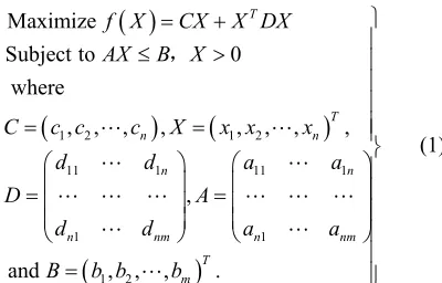
Let a quadratic programming problem be represented by
1 2 1 2
11 1 11
1 1
1 2 Maximize
Subject to 0
where
, , , , ,
,
and , , , .
T
n
n nm
T m
f X CX X
AX B X
C c c c X x x
d d
D A
d d
B b b b
1 , , T,
n n
n
n nm
DX
x
a a
a a
0 0 0 0
1, , ,2
T n
,
(1)
The matrix D is assumed symmetric and negative defi-nite. This means that f(X) is strictly concave. The con-straints are linear thus a convex solution space is guaran-teed. Any maximization quadratic model can be changed into a minimization and vice versa. This model is nonlinear and the idea is to linearize it in such a way that there is minimal complementary pivoting when solving.
3. Linearization of the Quadratic Problem
Let a quadratic programming problem be represented graphically as shown in Figure 1.
Where X x x x is the global optimum point.
This point X0 is not necessarily feasible and these vari- ables are not necessarily nonnegative. In other words they are free variables and Φ is the distance of the re-
(1)
(2)
(3)
f(x)
X0 X
Φ
···
(4) ···
0
( ) 0
[image:2.595.86.286.191.319.2]f X
Figure 1. Graphical representation of the quadratic pro-gramming problem.
quired optimal point X from X0 This distance is positive (Φ > 0)and when Φ = 0 then X0 is feasible and it is the trivial case. The planes (1), (2), (3), (4), ···, (m) are the linear constraints of the quadratic programming problem. The distance is the shortest distance from X0 to X.
3.1. Finding Point X0
The point X0 can easily be obtained from
0 0
1 1 1 1 1
0 0
2 2 2 2 2
0 0
n n n n n
x x x
x x x
x x x
(2) It is not necessary to solve for X0 own its own. The point X0 is represented by a set of Equation (2) in the linearized model.
3.2. Finding Point X
The point X is feasible and is not known and what are readily available are the limits of the variables. The lim-its for the variables are given by
0 0
(3)
where εj≥ 0.
This can also be represented as
X X X
1, , ,2
T n
(4) where
(5)
3.3. Nearness of Point X to X0 and the Objective Function
The point X becomes close to optimality when Φ is minimal. In other words we need to find the smallest value of Φ that gives a feasible point.
2 2 2
0 0 0
1 1 2 2 n n
x x x x x x
(6)
2 2 2
1 2 n
2
2 2 2 2
1 2 n
(7)
What minimizes also minimizes because ε≥ 0.
i.e.
2
2
(8) Theorem 1: What minimizes also minimizes. ε1 + ε2 + ··· + εn.
Proof: Let j j, then whatever minimizes
12 22 n2
1 2
Minimize n
also minimizes τ1 + τ2 + ··· + τn since τn
≥ 0.
The objective function of the linear model is:
This is the same as
Minimize T n I
ariables
0 0
(10) where In = (1, 1, ···, 1)T.
3.4. Linear Model for the Quadratic Function
0
0 0
0
Minimize Subject to
( ) 0
0, 0 and are free v
T n I
f X
X X X
AX B
X X
(11)
3.5. Redundant Constraints
In the linear model given above there are redundant con- straints and it is necessary to discard them without ne- cessarily losing the optimal point. The set of constraints given in (4) can be split into two inequality sets.
X X X
0
The first inequality set is given by
X X
0 0
XX
0
(12) (13) Similarly the second inequality set is
X X
0 0
XX
0 0
XX
0 0
XX
0
(14) (15) The set of inequalities in (15) are redundant.
Theorem 2: Whatever feasible solution that satisfies X
– X0 + Φ≥ 0 will also satisfy X – X0 – Φ≤ 0. Proof
Equality Case 1: If X – X0 + Φ = 0 then X – X0 – Φ = 0. If this is true then the following simultaneous equa-tions are feasible
(16) (17) This is possible when
X X
0
X X0
0
0
(18) (19) This is the trivial case. The equality case holds when
X = X0 and Φ = 0.
Inequality Case 2: Suppose Φ > 0 and we need to show that if X – X0 + Φ > 0 then X – X0 – Φ < 0.
If this is true then X – X0 + Φ > 0 is the same as (20)
Let X – X0 = Δ then the two inequalities become
(21)
0
0
0
0
Minimize Subject to
( ) 0
0
0, 0 and are free variables.
T n
I
f X
X X
AX B
X X
(22) Suppose Δ – Φ < 0 this implies Δ < Φ and this satisfies, –Δ – Φ < 0, whether Δ < 0 or Δ > 0 This implies that the second set of constraints can be discarded without losing the optimal point as they are redundant. The discarding also reduces the size of the LP significantly.
3.6. Reduced Linear Model
(23)
T n
The solution given by the linear model (23) is not necessarily optimal to the original quadratic problem.
4. Optimality and Linear Model
The solution to (23) becomes optimal if it also satisfies the necessary KKT conditions. In other words there is a need to fuse (23) and KKT conditions.
Reduced linear modelKKT conditions
I
DXATT Y C Minimize
A
Subject to X V B
0
( ) 0
f X
(24a)
0 0
X X
Where
Non-negativity conditions:
Y≥ 0, V≥ 0 and μ≥ 0.
AX B (24b) Complementary slackness:
YTX = 0 and μV = 0.
Expressions (24a) and (24b) can be represented as just (24).
Linear Model
The linear model becomes
0
0
Minimize Subject to
( ) 0
0
T n
T T
I
f X
X X
AX V B
DX A Y C
0
T
Y X V
(25)
where X≥ 0, Φ≥ 0, Y≥ 0, V≥ 0, μ≥ 0 and X0 are free variables.
Solving (25) will give a solution that is near optimal. Complementary slackness
(26)
If the solution given in (25) satisfies the complemen-tary slackness conditions then it is optimal. The comple-mentary slackness conditions cause a restricted basis entry for the simplex-method and this has significant effect on its speed. The idea or strategy in this paper is to find a feasible point closest to X0 and at the same time satisfying all the KKT conditions except the comple-mentary slackness conditions given in (26). The feasible point is then tested to see if it satisfies KKT or not. If it does then it is optimal else switch to complementary piv-ots or Wolfe’s method [14] until all the necessary condi-tions are satisfied.
5. Proposed Approach
The steps for the proposed approach are summarized as follows:
Step 1: Solve the linear model: Minimize T
n I
0
( ) 0
f X
0 0
XX
Subject to
AX V B
TT Y C
2 2
2 1 2
2 2
DX A
Step 2: If solution in Step 1 satisfies YTX = 0 and μV =
0 then it is optimal else go to Step 3.
Step 3: Use the optimal tableau in Step 1, switch to complementary pivots until all the necessary KKT condi-tions are satisfied.
6. Numerical Illustration
Use the proposed approach to linearize the following quadratic programming problem and then solve for the optimal solution.
1 2 1
1 2
1 2
1 2
Maximize 2 2 Subject to
6 9
2 7 12
, 0
x x x
x x
x x
x x
x x x
1 2
0 0
1 2
0 0
1 2
0
1 1 1
0
2 2 2
1 2 1
1 2 2
1 2 1 2 1
1 2 1 2 2
1 2 1 2 1 2 1 2
Minimize Subject to
2 2 2
2 4 2
0 0
6 9
2 7 12
2 2 2 2
2 4 6 7 2
Where , , , , , , , 0
x x
x x
x x
x x
x x v
x x v
x x y
x x y
v v y y
(27)
This is a portfolio selection problem where xj is the
number of millions of dollars invested in stock j. In this problem the objective is to obtain a minimum variance portfolio yielding the company’s expected desired return. This objective is obtained by solving the company’s quadratic problem formulated as (27).
Solution
The linear model is
(28)
0 0 1,
x x2
1 1 2 2 1 1 2 2 0
x y x y v v
are the free variables. The slackness conditions are
1 1.8 and 2 1.2
x x
(29) Solving (28) using the simplex-method we have
(30)
This solution satisfies the complementary slackness conditions and is optimal
In terms of the original problem the company must invest 1.8 million dollars in stock 1 and 1.2 million dol-lars in stock 2.
7. Conclusion
The strength of the approach presented in this paper lies within the simplicity with which linear models can be solved when there are no complementary conditions. The simplex-method performs efficiently if there is no re-stricted basis entry. The proposed approach significantly reduces the number of restricted basis iterations to the extent of even avoiding them completely in some prob-lems. This is a big advantage as complementary pivot algorithm will take roughly eight times as longer time to solve a quadratic program than the full speed simplex- method solving a linear problem of the same size.
REFERENCES
[1] S. Burer and D. Vandenbussche, “A Finite Branch-and- Bound Algorithm for Nonconvex Quadratic Programs with Semidefinite Relaxations,” Mathematical Program-ming, Series A, Vol. 113, No. 2, 2008, pp. 259-282. doi:10.1007/s10107-006-0080-6
[2] S. Burer and D. Vandenbussche, “Globally Solving Box- Constrained Nonconvex Quadratic Programs with Semi- definite-Based Finite Branch-and-Bound,” Computational Optimization and Applications, Vol. 43, No. 2, 2009, pp. 181-195.
[4] S. T. Liu and R.-T. Wang, “A Numerical Solution Meth-ods to Interval Quadratic Programming,” Applied Mathe-matics and Computation, Vol. 189, No. 2, 2007, pp. 1274-1281. doi:10.1016/j.amc.2006.12.007
[5] B. A. McCarl, H. Moskowitz and H. Furtan, “Quadratic Programming Applications,” Omega, Vol. 5, No. 1, 1977, pp. 43-55. doi:10.1016/0305-0483(77)90020-2
[6] J. J. Moré and G. Toraldo, “Algorithms for Bound Con-strained Quadratic Programming Problems,” Numerische Mathematik, Vol. 55, No. 4, 1989, pp. 377-400.
doi:10.1007/BF01396045
[7] G. B. Dantzig, “Linear Programming and Extensions,” Princeton University Press, Princeton, 1998.
[8] X.-W. Liu and Y.-X. Yuan, “A Null-Space Primal-Dual Interior-Point Algorithm for Nonlinear Optimization with Nice Convergence Properties,” Mathematical Program-ming, Vol. 125, No. 1, 2010, pp. 163-193.
doi:10.1007/s10107-009-0272-y
[9] S. Carvalho and A. Oliveira, “Interior-Point Methods
Applied to the Predispatch Problem of a Hydroelectric System with Scheduled Line Manipulations,” American Journal of Operations Research, Vol. 2, No. 2, 2012, pp. 266-271. doi:10.4236/ajor.2012.22032
[10] W.-Y. Sun and Y.-X. Yuan, “Optimization Theory and Methods: Nonlinear Programming,” Springer, New York, 2006.
[11] O. K. Gupta, “Applications of Quadratic Programming,”
Journal of Information and Optimization Sciences, Vol. 16, No. 1, 1995, pp. 177-194.
[12] R. Horst, P. M. Pardalos and N. V. Thoai, “Introduction to Global Optimization: Nonconvex Optimization and its Applications,” 2nd Edition, Kluwer Academic Publishers, Dordrecht, 2000.
[13] H. A. Taha, “Operations Research: An Introduction,” 9th Edition, Pearson, 2011.