Multivariable Regression Analysis for Optimised Mass Calculation of MEX 3D Printed Parts

(1)

Multivariable Regression Analysis for Optimised Mass Calculation of MEX

3D Printed Parts

C.V. DOICIN1_{, M.E. ULMEANU}1_{, A.E.W. RENNIE}2_{, E. LUPEANU}3 1_{University POLITEHNICA of Bucharest, Bucharest, Romania}

2_{Lancaster University, Engineering School, Lancaster, UK}

3_{National Institute of Geriatrics and Gerontology “Ana Aslan”, Bucharest, Romania}

[email protected], [email protected], [email protected],

[email protected]

ABSTRACT

Since its introduction in the early 1990s Material Extrusion (MEX) has become the most popular additive manufacturing technology for a variety of applications. One of the reasons of its popularity amongst users is the affordability of the equipment, materials and the open source software. Given the large variety of combinations optimisation of MEX process parameters can be quite elaborate. The paper provides a method for optimisation of mass calculation using multivariable regression analysis. Layer thickness, printing temperature and printing speed were considered the independent variables for a two level factorial experimental program. DOE was used to plan 12 sets of programs, out of which four were found to have significant models. The four models were validated through measured and calculated responses.

KEYWORDS: Optimised Mass Calculation, Regression Analysis, Material Extrusion, Design Of Experiments

1. INTRODUCTION

Material Extrusion (MEX) is the most widespread Additive Manufacturing (AM) technology, followed by Selective Laser Sintering (SLS) and Stereolithography (SLA) [1, 2]. MEX adoption has known a consistent increase over the last few years, using PLA as the most common material, followed by ABS [2]. As MEX application areas expand [1] the need arises to optimise printing process parameters in relation to certain goals, amongst which can be mentioned: print time, final part quality and costs. Some of the most significant process parameters considered as influencing MEX are the layer thickness, printing temperature and printing speed [3, 4, 5]. Print orientation, infill and raster angle have also been shown to highly influence final part properties [5, 6, 7]. Optimisation of process parameters specific to certain goals is quite complex, given the large variety of possible combinations provided by slicing software. Using DOE the current research optimises the calculation of mass for natural PLA 3D printed specimens, considering the variation of three process parameters.

Most available slicing software offer a rough estimate on the final mass of the 3D printed parts, making it hard to use as an input variable into other processes. The results of the paper can be useful in AM areas wher material costs are quite high and final part mass is important in overall fit and evaluation of the corresponding assemblies.

(2)

or response variables [8]. This type of statistical model has been previously used to attempt to assess the relationship between a number of variables, especially in the medical field for statistical processing of large volume data [9].

2. METHODS AND MATERIALS

The goal of the present research is to determine a more accurate method for mass calculation of MEX 3D printed parts, using multivariable regression analysis (MRA) to establish the relation of mass as a function of printing parameters. MRA entails several stages, as follows: 1. Establish the form of the regression function; 2. Establish the structure of the experimental program using design of experiments (DOE); 3. Calculate the regression coefficients; 4. Verify the regression functions’ form suitability and the significance of the regression coefficients; 5. Determine the statistical errors; 6. Determine the confidence intervals. MRA was undertaken using Design-Expert® V11 Software by defining the form of the function and the experimental program type. By running the software a mathematical expression was determined, in order to define the dependency between the final mass of 3D printed specimens and three process parameters: layer thickness (s, mm), printing temperature (t, degrees) and printing speed (v, mm/min). In this case, the mass is considered the main dependent variable and the three process parameters are the input independent natural variables. Due to the combination between the independent variables in relation to the dependent variable, a factorial experimental program was defined, with two variation levels (23 _{type), with the medium values determined as the} arithmetic average of the minimum and maximum limits. Three control experiments were used, leading to a base experimental program of 11 experiments. Four PLA filament type materials were considered for DOE, from four different manufacturers. Natural filaments were chosen in order to exclude changes in material properties due to various pigments. Three ISO test standards were used to print the specimens in one direction, as follows: ISO 527 – tensile test specimens printed horizontally; ISO 179 – flexural test specimens printed normal; ISO 178 – Charpy impact test specimens printed normal.

Considering four material types, three specimen test standards, one orientation and a factorial experimental program with three controls, the final number of undertaken experiments was set to 132. The variation levels for the three aforementioned process parameters are listed in Table 1. The limit values were set in accordance with the four different manufacturers’ requirements. MRA was run by coding the natural variables, as presented in Table 2.

Table 1: Variation levels for the independent natural variables

No.

Crt. Independent variable Minimum Medium Maximum

1 Layer thickness – s [mm] 0.10 0.15 0.20

2 Printing temperature – t[o_] ₂₀₀o ₂₁₀o ₂₂₀o

3 Printing speed – v [mm/min] 40 mm/min 60 mm/min 80 mm/min

(3)

[image:3.595.72.527.89.254.2]

Table 2: Design of experiments for three variables– Base experimental program

Experiment

No. s [mm] Natural variables t[o_] _v_[mm/min] _A Coded variables _B _C

E1. 0.15 210 60 0 0 0

E2. 0.10 200 40 -1 -1 -1

E3. 0.10 200 80 -1 -1 +1

E4. 0.10 220 40 -1 +1 -1

E5. 0.10 220 80 -1 +1 +1

E6. 0.15 210 60 0 0 0

E7. 0.20 220 80 +1 +1 +1

E8. 0.20 220 40 +1 +1 -1

E9. 0.20 200 80 +1 -1 +1

E10. 0.20 200 40 +1 -1 -1

E11. 0.15 210 60 0 0 0

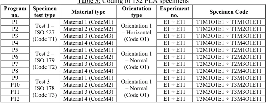
[image:3.595.70.525.330.507.2]

Manufacturing of the 132 specimens needed 12 process data sheets following the encoding proposed in Table 3. Each batch of 11 specimens are printed on the same 3D printer in order to ensure the repeatability of the process parameters.

Table 3: Coding of 132 PLA specimens

Program

no. Specimen test type Material type Orientation type Experiment no. Specimen Code

P1 _{Test 1 –} ISO 527 (Code T1)

Material 1 (CodeM1) Orientation 1 – Horizontal (Code O1)

E1 ÷ E11 T1M1O1E1 ÷ T1M1O1E11

P2 Material 2 (CodeM2) E1 ÷ E11 T1M2O1E1 ÷ T1M2O1E11

Material 1 (CodeM1) Orientation 1 – Normal (Code O1)

E1 ÷ E11 T2M1O1E1 ÷ T2M1O1E11

Material 1 (CodeM1) Orientation 1 – Normal (Code O1)

E1 ÷ E11 T3M1O1E1 ÷ T3M1O1E11

3. RESULTS AND DISCUSSIONS

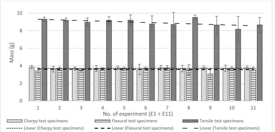
Gcodes for all specimens were prepared using Cura 3.4 software, which gave a mass estimation of 10g for the tensile test specimens and 4g for both flexural and Charpy impact test specimens. Mass estimations are given by the Cura 3.4 software considering the filament diameter and a standard material type density. As, all PLA materials have the same material density input, the mass calculation will always be the same, regardless of the chemical composition of each material batch. Regardless of the changes in printing parameters, according to Table 2, the same two mass values were estimated by the software.

132 PLA material specimens were 3D printed and weighted individually using an analytical scale with a 0,0001 g precision (Figure 1).

(4)

[image:4.595.77.519.92.296.2]

Figure 1: Example of coded specimens – a) tensile test specimens printed horizontally from M1; b) flexural test specimens printed normal from M2; c) Charpy impact test specimens printed normal from M3; d) weighing of tensile test specimen printed horizontally from M4

Figure 2: Average mass for 132 specimens for 11 experiment types

In order to accurately express the dependency of the printed parts’ mass to the three independent variables, each of the 12 previously defined programs (Table 3) were subjected to a multivariable regression analysis using Design-Expert® V11 Software (Figure 3).

A natural logarithmic transformation was used to process all 132 responses. The final equations in terms of coded factors have the following general form:

𝑙𝑙𝑙𝑙(𝑚𝑚) =𝑎𝑎0+𝑎𝑎1∙ 𝐴𝐴+𝑎𝑎2∙ 𝐵𝐵+𝑎𝑎3∙ 𝐶𝐶+𝑎𝑎12∙ 𝐴𝐴 ∙ 𝐵𝐵+𝑎𝑎13∙ 𝐴𝐴 ∙ 𝐶𝐶+𝑎𝑎23∙ 𝐵𝐵 ∙ 𝐶𝐶+𝑎𝑎123∙ 𝐴𝐴 ∙ 𝐵𝐵 ∙ 𝐶𝐶 (1)

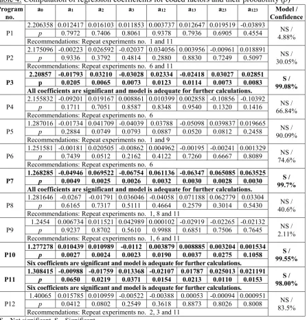
All eight regression coefficients for the 12 programs are listed in Table 4.

0 2 4 6 8 10

1 2 3 4 5 6 7 8 9 10 11

M

as

s [g

]

No. of experiment (E1 ÷ E11)

[image:4.595.70.528.357.577.2]

(5)

[image:5.595.101.496.69.269.2]

Figure 3: Input data for program P1 using Design-Expert® V11 Software

Table 4: Computation of regression coefficients for coded factors and their probability (p)

Program

no. a0 a1 a2 a3 a12 a13 a23 a123 Confidence Model /

P1 2.206358 0.012417 0.016103 0.011853 0.003737 0.012647 0.019519 -0.03893 p 0.7972 0.7406 0.8061 0.9378 0.7936 0.6905 0.4554 _4.88%NS / Recommendations: Repeat experiments no. 1 and 11

P2 2.175096 -0.00223 0.026592 -0.02037 0.034056 0.003956 -0.00961 0.018891 p 0.9336 0.3792 0.4814 0.2880 0.8830 0.7249 0.5097 _30.05%NS / Recommendations: Repeat experiments no. 6 and 11

P3 2.20857 -0.01793 0.03210 -0.03028 0.02334 -0.02418 0.03027 0.02851 p 0.0205 0.0065 0.0073 0.0123 0.0114 0.0073 0.0083 _99.08%S / All coefficients are significant and model is adequate for further calculations.

P4 2.155832 -0.09201 0.019167 0.008861 0.010399 0.002858 -0.10856 -0.10392 p 0.1711 0.7051 0.8587 0.8348 0.9540 0.1320 0.1416 _66.84%NS / Recommendations: Repeat experiments no. 6

P5 1.287016 -0.01734 0.041709 -0.04039 0.03788 -0.05098 0.039837 0.019665 p 0.2884 0.0749 0.0793 0.0887 0.0520 0.0812 0.2458 _90.09%NS / Recommendations: Repeat experiments no. 1 and 9

P6 1.251581 -0.00181 0.020505 -0.00862 0.004962 -0.00195 -0.00241 0.001329 p 0.7439 0.0512 0.2162 0.4122 0.7260 0.6667 0.8089 _74.6%NS / Recommendations: Repeat experiments no. 6

P7 1.268285 -0.04946 0.069522 -0.06754 0.061136 -0.06347 0.065085 0.063525 p 0.0049 0.0025 0.0026 0.0032 0.0030 0.0028 0.0030 _99.7%S / All coefficients are significant and model is adequate for further calculations.

P8 1.281646 -0.0267 -0.01791 0.036046 -0.04058 0.071188 0.062779 0.03304 p 0.6165 0.7317 0.5111 0.4664 0.2579 0.3014 0.5430 _40.6%NS / Recommendations: Repeat experiments no. 1, 8 and 11

P9 1.2454 0.006734 0.011521 0.042989 0.000102 -0.02919 -0.02265 -0.02132 p 0.9237 0.8702 0.5610 0.9988 0.6851 0.7506 0.7645 _2.11%NS / Recommendations: Repeat experiments no. 1, 6 and 11

P10 1.277278 0.010439 0.010989 -0.0112 0.003879 0.008885 0.003204 0.001534 p 0.0027 0.0024 0.0023 0.0190 0.0037 0.0275 0.1058 _99.55%S / Six coefficients are significant and model is adequate for further calculations.

P11 1.308415 -0.00988 -0.01759 0.013368 -0.02107 0.01787 0.025013 0.021191 p 0.0650 0.0219 0.0371 0.0154 0.0213 0.0110 0.0153 _98.00%S / Six coefficients are significant and model is adequate for further calculations.

P12 1.40065 0.015785 0.010959 -0.00522 -0.00388 0.00053 -0.00094 0.000951 p 0.0412 0.0802 0.2549 0.3618 0.8873 0.8026 0.8008 _83.5%NS / Recommendations: Repeat experiments no. 2, 3 and 11

[image:5.595.79.527.295.763.2]

(6)

Regression coefficients are significant if they have a probability p < 0.05. The model is significant relative to the noise if the majority of the coefficients have a probability value under 0.05 and the confidence is above the standard value. The analysis was run with a two sided interval and a standard confidence of 95%. Model inadequacies arise from too scattered central point values.

The final equation in terms of actual factors have the general form set by relation (2). Using expression (2) and the coefficient values provided in Table 5, the calculated responses are summarised in Table 5 for the significant programs.

𝑙𝑙𝑙𝑙(𝑚𝑚) =𝑏𝑏0+𝑏𝑏1∙ 𝑠𝑠+𝑏𝑏2∙ 𝑡𝑡+𝑏𝑏3∙ 𝑣𝑣+𝑏𝑏12∙ 𝑠𝑠 ∙ 𝑡𝑡+𝑏𝑏13∙ 𝑠𝑠 ∙ 𝑣𝑣+𝑏𝑏23∙ 𝑡𝑡 ∙ 𝑣𝑣+𝑏𝑏123∙ 𝑠𝑠 ∙ 𝑡𝑡 ∙ 𝑣𝑣 (2)

Table 5: Regression coefficients for non-coded factors

Program

no. b0 b1 b2 b3 b12 b13 b23 b123

[image:6.595.70.531.338.513.2]

P3 -0.5488632 27.2089437 0.01278318 0.06012228 -0.124367 -0.62281845 -0.000276 0.00285067 P7 -4.4661735 57.1830074 0.02625820 0.13790691 -0.258876 -1.39748544 -0.000627 0.00635246 P10 1.28515438 -0.02101646 0.00035423 -0.0004268 -0.001444 -0.02332026 -6.9820·10-6 _0.00015336 P11 -1.9284124 34.2801101 0.01612945 0.03847543 -0.169285 -0.42713707 -0.0001928 0.00211908

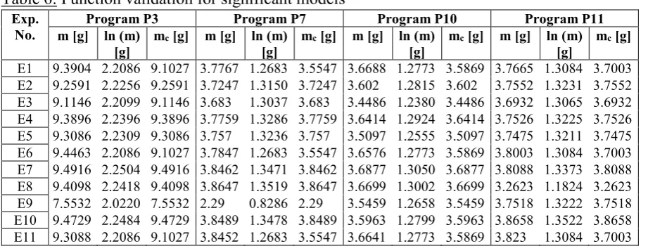
Table 6: Function validation for significant models

Exp.

No. m [g] ln (m) Program P3 Program P7 Program P10 Program P11

[g] mc [g] m [g] ln (m) [g] mc [g] m [g] ln (m) [g] mc [g] m [g] ln (m) [g] mc [g]

E1 9.3904 2.2086 9.1027 3.7767 1.2683 3.5547 3.6688 1.2773 3.5869 3.7665 1.3084 3.7003 E2 9.2591 2.2256 9.2591 3.7247 1.3150 3.7247 3.602 1.2815 3.602 3.7552 1.3231 3.7552 E3 9.1146 2.2099 9.1146 3.683 1.3037 3.683 3.4486 1.2380 3.4486 3.6932 1.3065 3.6932 E4 9.3896 2.2396 9.3896 3.7759 1.3286 3.7759 3.6414 1.2924 3.6414 3.7526 1.3225 3.7526 E5 9.3086 2.2309 9.3086 3.757 1.3236 3.757 3.5097 1.2555 3.5097 3.7475 1.3211 3.7475 E6 9.4463 2.2086 9.1027 3.7847 1.2683 3.5547 3.6576 1.2773 3.5869 3.8003 1.3084 3.7003 E7 9.4916 2.2504 9.4916 3.8462 1.3471 3.8462 3.6877 1.3050 3.6877 3.8088 1.3373 3.8088 E8 9.4098 2.2418 9.4098 3.8647 1.3519 3.8647 3.6699 1.3002 3.6699 3.2623 1.1824 3.2623 E9 7.5532 2.0220 7.5532 2.29 0.8286 2.29 3.5459 1.2658 3.5459 3.7518 1.3222 3.7518 E10 9.4729 2.2484 9.4729 3.8489 1.3478 3.8489 3.5963 1.2799 3.5963 3.8658 1.3522 3.8658 E11 9.3088 2.2086 9.1027 3.8452 1.2683 3.5547 3.6641 1.2773 3.5869 3.823 1.3084 3.7003 m – measured response, mc – calculated response

The proposed models have been validated with a precision of 0,0001g in relation to the measured response values.

4. CONCLUSIONS

(7)

The applicability of the method includes medium to large scale production of parts, especially in industries where materials are quite expensive and mass variation has an important influence on final costs. Jewellery and medical/ dental applications are some of the most appropriate for further development of the optimisation method, due to relatively reduced overall weight of the finished parts and high costs of the materials.

Further research includes validation of the method by manufacturing parts with various geometries using printing parameter values set in the significant programs.

ACKNOWLEDGEMENT

Erasmus+ Project Nr. 2018-1-RO01-KA203-049511, “TecHnology and EntrepreneUrship Education - Bridging the Gap for Smart Product Development” - TecHUB 4.0, 2018 – 2020.

REFERENCES

[1]. Moreau C., The state of 3D printing 2018, Sculpteo Annual Report, 2018.

[2]. 3D Hubs, Online Manufacturing Trends Q4/ 2018, available at:

https://www.3dhubs.com/trends, Last accessed: 28.01.2019.

[3]. H. Li, T. Wang, J. Sun and Z. Yu, The effect of process parameters in fused deposition modelling on bonding degree and mechanical properties, Rapid Prototyping Journal, 2017, 24 (1), pp.80-92.

[4]. J.M. Chacón, M.A. Caminero, E. García-Plaza and P.J. Núñez, Additive manufacturing of PLA structures using fused deposition modelling: Effect of process parameters on mechanical properties and their optimal selection, Materials & Design, 2017, 124, pp.143-157.

[5]. A.P. Gordon, J. Torres, M. Cole, A. Owji and Z. DeMastry, An approach for mechanical property optimization of fused deposition modeling with polylactic acid via design of experiments, Rapid Prototyping Journal, 2016, 22(2), pp.387-404.

[6]. T. Nancharaiah, Optimization of Process Parameters in FDM Process Using Design of Experiments, International Journal on Emerging Technologies, 2011, 2(1), pp.100-102

[7]. A. Kohad, R. Dalu, Optimization of Process Parameters in Fused Deposition Modeling: A Review, International Journal of Innovative Research in Science, Engineering and Technology, 2017, 6(1), pp.505-511.

[8]. B. Hidalgo, M. Goodman, Multivariate or Multivariable Regression, American Journal of Public Health, 2013, 103(1), pp.39-40.