Early science with the Large Millimetre Telescope:New mm wave detections of circumstellar discs in IC 348 from LMT/AzTEC

Advance Access publication 2019 July 03

Early science with the Large Millimetre Telescope: new mm-wave

detections of circumstellar discs in IC 348 from LMT/AzTEC

Michael S. Petersen ,

Robert A. Gutermuth,

Erick Nagel,

Grant W. Wilson

and James Lane

1_{Department of Astronomy, University of Massachusetts at Amherst, 710 N. Pleasant St, Amherst, MA 01003, USA}

2_{Department of Astronomy, Universidad de Guanajuato, Guanajuato, Gto 36240, Mexico}

3_{Physics Department, Lancaster University, Lancaster LA1 4YQ, UK}

Accepted 2019 June 14. Received 2019 June 13; in original form 2018 November 2

A B S T R A C T

We present the most complete sample of mm measurements of protoplanetary discs in the star-forming region IC 348 to date. New observations from the Large Millimetre Telescope and the 1.1 mm camera AzTEC are combined with literature results in order to characterize the disc population as relating to both stellar properties within the IC 348 region and across other star-forming regions. In addition to detecting 28 of 116 observed known infrared-excess sources, we detected emission from two previously unknown candidate transition discs in the region. When combined with literature results, we find evidence for a steeper-than-expected slope, on average, in disc spectral energy distributions at millimetre wavelengths in the IC 348 region. We show that the presence or absence of high-mass discs is a sensitive indicator of regional evolution, both among star-forming regions and within IC 348. In contrast, low-mass

discs exhibit almost no apparent evolution within the first∼5 Myr when compared among

regions.

Key words: planets and satellites: individual: protoplanetary discs – stars: protostars – stars: rotation.

1 I N T R O D U C T I O N

Pre-main-sequence stars commonly possess dusty, gas-rich circum-stellar discs, and it is broadly believed that these discs are the birthplaces of planets. Observations of protoplanetary circumstellar discs in the infrared reveal the presence of warm inner discs, where the accreting material for the star’s continued growth resides (see

Espaillat et al.2014 for a review). However, models of infrared

observations are degenerate in determining disc mass due to the optically thick nature of the hot inner disc, which complicates the determination of dust temperature, geometry, and composition

(Espaillat et al.2012). The majority of the mass is hosted in an outer

disc, where large dust grains reside; the outer disc is most efficiently imaged in the (sub-)millimetre (mm) where the dust emission is generally optically thin and thus a good tracer of mass.

Over the past 10 yr, studies have sought to measure mm fluxes of protoplanetary discs to construct a timeline for circumstellar

disc evolution and planet formation (see Williams & Cieza2011;

Alexander et al. 2014, for reviews). Several regions have been

studied at millimetre wavelengths, including Taurus (Andrews

et al.2013), Lupus (Ansdell et al.2016), Chamaeleon I (Pascucci

_{E-mail:[email protected]}

et al. 2016), σ Ori (Ansdell et al. 2017), the Upper Scorpius

OB Association (Barenfeld et al. 2016), Orion (Eisner et al.

2016,2018), and the region studied here, IC 348 (Ru´ız-Rodr´ıguez

et al.2018). These studies have performed a linear regression to

characterize a relationship betweenMdust andM. Pascucci et al.

(2016) compiled data from∼1–3 Myr old regions (Taurus, Lupus,

and Chamaeleon I) to conclude that discs are in the fragmentation-limited regime (characterized by large pebbles undetectable in mm emission) owing to the steeper-than-linear relationship between

Mdust and M. In this paradigm, dust evolution proceeds on a

shorter time-scale around lower mass hosts. The conclusion of

a steeper-than-linear Mdust–M relationship was bolstered by the

subsequent finding of a steeper-than-linear relation in σ Ori by

Ansdell et al. (2017), albeit with large scatter (2+dex) inMdustat

a givenM. Observations of disc sizes, while still few in number,

suggest that older discs may be smaller in size than their young

counterparts (Barenfeld et al.2017), another possible explanation

for the steeper-than-linear relation. However, the relationship is far from well characterized, and the simple scalings proposed deserve scrutiny. Discs can evolve based on their environment, as has been shown through disc fraction variation in the infrared

(Muzerolle et al. 2010). Additionally, environmental effects are

difficult to quantify, owing to the small number of regions where

such studies are possible (Guarcello et al.2016). Subdivisions of

2019 The Author(s)

individual star formation regions may hold some promise in this regard.

Of the fields listed above, the young Taurus region (t∼1–2 Myr)

has been well studied as a result of proximity (d∼140 pc), boasting

a complete sample of 210 discs hosted by stars at spectral types

earlier than M8.5 (Andrews & Williams2005, Andrews et al.2013).

However, Taurus is both young and diffuse, and generally thought to not resemble the nurseries where most stars in the Milky Way are born.

IC 348 is generally described from pre-main-sequence age

estimates as a young post-embedded cluster (t∼2–3 Myr, Luhman

et al.2003), though recent works have argued for an older age for

IC 348 (6 Myr, Bell et al.2013, Cottaar et al.2014). Known to host

circumstellar disc-bearing Class II young stellar objects (YSOs)

by infrared analysis (Lada et al.2006; Muench et al.2007; Rebull

et al.2007; Jørgensen et al.2008; Evans et al.2009; Gutermuth

et al.2009), the evolution of the circumstellar discs in IC 348 has

been probed using both disc fraction arguments as well as disc spectral energy distribution (SED) studies. The distance of IC 348,

measured as 315 pc in Muench et al. (2007),d=273 ±23 pc

(Ripepi et al.2014), 321±10 pc from VLBA (Ortiz-Le´on et al.

2018), and∼320 pc fromGaiadata (Ortiz-Le´on et al.2018;

Ru´ız-Rodr´ıguez et al.2018) has made the region a prime target for study

and comparison with Taurus. The value of comparing to IC 348 is not just age, but also environmental difference. IC 348 is older and denser, and centred on an intermediate-mass system (HD 281159,

classified as a B5 binary system in Luhman et al.2003) whose

far-ultraviolet (FUV) flux could substantially erode the outer discs

of members that get too close (Adams et al.2006). Until recently,

information about disc masses in IC 348 had only been measured in

20 objects (Lee, Williams & Cieza2011; Espaillat et al.2012; Cieza

et al.2015), leaving the disc mass function largely unconstrained.

Andrews et al. (2013) found that with the then-current sample of

disc masses in IC 348, there was no appreciable difference between Taurus and IC 348, but noted that this may be affected by the lack of completeness in the latter. With more information, Ru´ız-Rodr´ıguez

et al. (2018) demonstrated a rudimentary difference between Taurus

and IC 348 that they attribute to the age of the system. While

Ru´ız-Rodr´ıguez et al. (2018) detected 40 discs using ALMA, more than

half of the systems classified as Class II do not have detectable millimetre emission in their paper. Clearly, obtaining the most complete census of disc masses in IC 348 is then of the utmost importance for determining a possible evolutionary timeline as well as for constraining environmental impacts on disc evolution. Fully characterizing the disc population of a star-forming region such as IC 348 will add more data to constrain typical disc lifetimes,

generally thought to be∼3 Myr, with estimates as low as 1 Myr and

as high as 10 Myr (Strom et al.1989; Haisch Jr., Lada & Lada2001;

Hillenbrand2005; Mamajek2009; Muzerolle et al.2010; Pfalzner,

Steinhausen & Menten2014).

In this paper, we present an analysis of the disc mass properties of IC 348 based on a unification of extant data in the literature with a new survey to determine the disc masses in IC 348 using the Large Millimetre Telescope (LMT) atop Volcan Sierra Negra, in Puebla,

Mexico, and the 1.1 mm camera AzTEC (Wilson et al.2008). In

Section 2, we describe the new observations and subsequent data reduction, as well as ancillary data sources. We present results using the new data in Section 3, culminating in the most complete list of disc masses measured at mm wavelengths in IC 348 to date. In Section 4, we use ancillary data relating to stellar host properties to study the dependence of disc mass on stellar parameters. Section 4 focuses on the relationships between mm flux and stellar properties.

We compare our findings to the Taurus sample of Andrews et al.

(2013) in Section 5 before discussing the potential implications for

disc evolutionary models. We summarize in Section 6.

2 O B S E RVAT I O N S

In this section, we begin by describing the target selection in IC 348. We then overview the combined AzTEC and LMT system as it pertains to observations of the IC 348 region and describe the method by which sources were extracted in Section 2.2. We describe sources of ancillary data in Section 2.3 and the matching of ancillary sources to LMT sources in Section 2.4 .

2.1 Target selection

Our AzTEC observations are centred on known

mid-IR-excess-bearing YSO targets in IC 348 from Gutermuth et al. (2009). Fig.1

is the J versus J–H colour–magnitude diagram for all such sources in IC 348, and regions are drawn with dashed lines to show mass- and extinction-limited sample areas. The original sample region named

T1 requires sources withM>0.09 M(using Baraffe et al.2015

isochrones) andAV< 5 mag. We adopted T1 for our target field

selection. We successfully obtained maps of 53 of 60 target fields

that covered all Gutermuth et al. (2009) identified 62 YSOs in this

region. As discussed in Section 2.2 below, we expanded the masked field of view of each map in order to explore lower sensitivity areas of coverage further from the target centre point. This considerably augmented our spatial coverage, and the added areas have only modestly lower sensitivity. In total, we achieved quality detections and limits for all 62 YSOs in region T1. Furthermore, if we consider

a more generous mass- and extinction-limited region of Fig.1, such

as region T2 where sources must have M>0.05 M andAV <

8 mag, we have detections or useful limits for 90/97 YSOs in this region, over 90 per cent coverage.

2.2 Data acquisition

The data were collected using the 144-element 1.1 mm bolometer

array AzTEC (Wilson et al.2008) on the 50-m diameter LMT during

its early science phase when it was limited to a 32-m diameter collecting area. The detailed survey information is summarized in

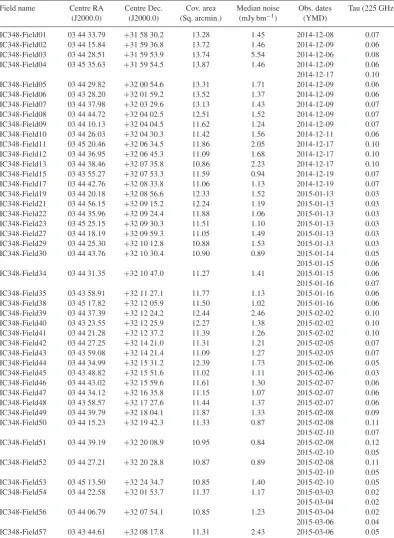
Table1. The LMT observatory employs a dynamic queue strategy to

maximize the use of AzTEC during the best observing conditions.

The τ measured during our observations was 0.02 to 0.12. We

observed our targets using ‘photometry mode’, a Lissajous scanning pattern that is designed to produce uniform, maximal sensitivity in the central 30 arcsec area. Within this maximal sensitivity region, our detection rate of primary targets was limited. Thus, we lowered the coverage threshold in the pipeline to 10 per cent of the median coverage of the map (default is 90 per cent), expanding the resultant field of view several fold and achieving reasonable sensitivity for serendipitous observations of many more disc-bearing and discless IC 348 members. The typical median noise level of the final

expanded coverage maps is ∼1 mJy per beam RMS, and we

consistently achieve a factor of 2–4 less than that in the central high coverage zones. Noise levels are estimated directly from the

time stream data using a jackknifing technique (Scott et al.2008).

AzTEC has been a guest instrument on other telescopes, and we calibrate data from AzTEC on LMT in a similar fashion to these

earlier observing campaigns (e.g. Scott et al.2008). In summary,

observers obtain load curves and beam maps 2–3 times per night and pointing offset observations were taken every hour. The primary flux

Table 1. LMT/AzTEC observations table.

Field name Centre RA Centre Dec. Cov. area Median noise Obs. dates Tau (225 GHz) (J2000.0) (J2000.0) (Sq. arcmin.) (mJy bm−1_{) (YMD)}

IC348-Field01 03 44 33.79 +31 58 30.2 13.28 1.45 2014-12-08 0.07

IC348-Field02 03 44 15.84 +31 59 36.8 13.72 1.46 2014-12-09 0.06

IC348-Field03 03 44 28.51 +31 59 53.9 13.74 5.54 2014-12-06 0.08

IC348-Field04 03 45 35.63 +31 59 54.5 13.87 1.46 2014-12-09 0.06

2014-12-17 0.10

IC348-Field05 03 44 29.82 +32 00 54.6 13.31 1.71 2014-12-09 0.06

IC348-Field06 03 43 28.20 +32 01 59.2 13.52 1.37 2014-12-09 0.06

IC348-Field07 03 44 37.98 +32 03 29.6 13.13 1.43 2014-12-09 0.07

IC348-Field08 03 44 44.72 +32 04 02.5 12.51 1.52 2014-12-09 0.07

IC348-Field09 03 44 10.13 +32 04 04.5 11.62 1.24 2014-12-09 0.07

IC348-Field10 03 44 26.03 +32 04 30.3 11.42 1.56 2014-12-11 0.06

IC348-Field11 03 45 20.46 +32 06 34.5 11.86 2.05 2014-12-17 0.10

IC348-Field12 03 44 36.95 +32 06 45.3 11.09 1.68 2014-12-17 0.10

IC348-Field13 03 44 38.46 +32 07 35.8 10.86 2.23 2014-12-17 0.10

IC348-Field15 03 43 55.27 +32 07 53.3 11.59 0.94 2014-12-19 0.07

IC348-Field17 03 44 42.76 +32 08 33.8 11.06 1.13 2014-12-19 0.07

IC348-Field19 03 44 20.18 +32 08 56.6 12.33 1.52 2015-01-13 0.03

IC348-Field21 03 44 56.15 +32 09 15.2 12.24 1.19 2015-01-13 0.03

IC348-Field22 03 44 35.96 +32 09 24.4 11.88 1.06 2015-01-13 0.03

IC348-Field23 03 45 25.15 +32 09 30.3 11.51 1.10 2015-01-13 0.03

IC348-Field27 03 44 18.19 +32 09 59.3 11.05 1.49 2015-01-13 0.03

IC348-Field29 03 44 25.30 +32 10 12.8 10.88 1.53 2015-01-13 0.03

IC348-Field30 03 44 43.76 +32 10 30.4 10.90 0.89 2015-01-14 0.05

2015-01-15 0.06

IC348-Field34 03 44 31.35 +32 10 47.0 11.27 1.41 2015-01-15 0.06

2015-01-16 0.07

IC348-Field35 03 43 58.91 +32 11 27.1 11.77 1.13 2015-01-16 0.06

IC348-Field38 03 45 17.82 +32 12 05.9 11.50 1.02 2015-01-16 0.06

IC348-Field39 03 44 37.39 +32 12 24.2 12.44 2.46 2015-02-02 0.10

IC348-Field40 03 43 23.55 +32 12 25.9 12.27 1.38 2015-02-02 0.10

IC348-Field41 03 44 21.28 +32 12 37.2 11.39 1.26 2015-02-02 0.10

IC348-Field42 03 44 27.25 +32 14 21.0 11.31 1.21 2015-02-05 0.07

IC348-Field43 03 43 59.08 +32 14 21.4 11.09 1.27 2015-02-05 0.07

IC348-Field44 03 44 34.99 +32 15 31.2 12.39 1.73 2015-02-06 0.05

IC348-Field45 03 43 48.82 +32 15 51.6 11.02 1.11 2015-02-06 0.03

IC348-Field46 03 44 43.02 +32 15 59.6 11.61 1.30 2015-02-07 0.06

IC348-Field47 03 44 34.12 +32 16 35.8 11.15 1.07 2015-02-07 0.06

IC348-Field48 03 43 58.57 +32 17 27.6 11.44 1.37 2015-02-07 0.06

IC348-Field49 03 44 39.79 +32 18 04.1 11.87 1.33 2015-02-08 0.09

IC348-Field50 03 44 15.23 +32 19 42.3 11.33 0.87 2015-02-08 0.11

2015-02-10 0.07

IC348-Field51 03 44 39.19 +32 20 08.9 10.95 0.84 2015-02-08 0.12

2015-02-10 0.05

IC348-Field52 03 44 27.21 +32 20 28.8 10.87 0.89 2015-02-08 0.11

2015-02-10 0.05

IC348-Field53 03 45 13.50 +32 24 34.7 10.85 1.40 2015-02-10 0.05

IC348-Field54 03 44 22.58 +32 01 53.7 11.37 1.17 2015-03-03 0.02

2015-03-04 0.02

IC348-Field56 03 44 06.79 +32 07 54.1 10.85 1.23 2015-03-04 0.02

2015-03-06 0.04

IC348-Field57 03 43 44.61 +32 08 17.8 11.31 2.43 2015-03-06 0.05

calibrator and beam-mapping target was CRL618, and the pointing offset calibrator target was 3c111 for all fields. Pointing offsets drifted by 1.5–2 arcsec per hour. We interpolate pointing offsets between successive calibrator measurements, thus residual pointing

offsets should be<1 arcsec.

All the data were processed following the standard AzTEC data treatment, including ‘despiking’ of the signal time streams, low-pass filtering, and principal component analysis (PCA) atmospheric

filtering (Scott et al.2008) as implemented in the standard AzTEC

C++ data reduction pipeline. The final maps are produced by

applying adaptive Wiener filtering to the data. The goal is to produce and apply an optimized filter for detecting unresolved sources without sacrificing the excellent angular resolution of AzTEC and LMT (8.5 arcsec at 32-m diameter). The depth of our maps revealed a fair amount of residual low column density cloud structure, and the high default setting for the PCA filtering and the Wiener filtering created numerous false point sources within it. To attempt to more clearly distinguish between bona fide point sources and strongly

Figure 1. J versus J–H diagram for the YSO members of IC 348 that possess circumstellar discs as identified in Gutermuth et al. (2009). Objects with successful mm detections with LMT/AzTEC are plotted as squares, and those with quality upper limits are plotted as triangles. The small plot points mark those objects that were not covered by the LMT in our survey. For reference, we overlay the data with the 3 Myr pre-main-sequence stellar model isochrone of Baraffe et al. (2015) that spans masses of 0.01–1.4 M (curved solid line) and extinction vectors from Rieke & Lebofsky (1985) (straight solid lines with large asterisks atAV=0 and 10 mag) extending from masses of 0.3 and 0.08 M. The dashed lines mark the mass- and extinction-limited target sample areas T1 and T2, for reference.

filtered resolved emission, we performed a secondary filtering process on all the data, replacing the Wiener filter with a simple Gaussian filter of the same full width at half-maximum (FWHM) as the telescope beam (8.5 arcsec) and reducing the strength of the PCA filter to 3 from 9 eigenvectors. This treatment, named ‘soft filtering’ below to distinguish it from the ‘hard filtering’ of the standard process, is not optimized for point sources, and thus it does not achieve as low noise levels and it yields a marginal loss of angular resolution in the final images (12 arcsec FWHM). However, it is far less destructive to resolved emission, facilitating a fair evaluation of the nature of sources detected in both treatments.

We identify and extract point sources in the same manner as pre-stellar dense gas cores were extracted in another AzTEC/LMT

survey (Sokol et al.2019). In summary, each flux map is masked to

include those pixels that have sufficient S/N and coverage (2.5 and 10 per cent of median coverage, respectively), scaled by its median

noise value, inverted, and fed to the native IDL functionwatershed

to identify and merge regions of contiguous emission with some central peak. Saddle points in the flux distribution are also identified and used to split close sources. Reported positions are flux-weighted means of the pixels within the half-peak-power emission area, and point source fluxes and S/N are obtained from the locations of the observed peak flux values within each source footprint. We reject all source candidates whose footprints fall within 8 arcsec of the coverage edge to eliminate a large source of atmospheric filtration artefacts. The process to extract resolved structures from the soft filtering process is identical.

Once we have source catalogues derived from the two filtering methods’ images, the positions of all prospective point sources detected with strong filtering are checked for a resolved source in the soft filtering list. Where no match is found, an upper limit is extracted to ensure consistency with that source being lost in the elevated noise of the soft filtering. Where matches exist, source concentration (peak to total flux ratio, including a low S/N correction; Sokol et al., in preparation) derived from the soft filtering data and ratios of the peak fluxes from both methods are computed. We adopt an empirical limit that any object with a soft filtering counterpart must also have a peak to total flux ratio greater than 0.4, or else we consider that detection to be cloud-dominated and thus a poor representation of the disc flux. Where objects are cloud-dominated, the hard filtering flux is instead reported as an upper limit set by our inability to separate disc from cloud emission with confidence rather than by noise constraints. For all YSOs that have no detections under soft or hard filtering, we report three times the noise value of the nearest pixel position as our noise-bound upper limit.

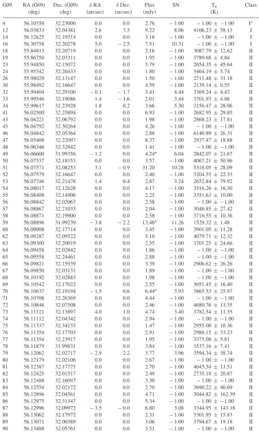
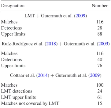
Using the YSO list of Gutermuth et al. (2009), we found that 116

total source positions had been covered, of the complete sample

of 160 in Gutermuth et al. (2009). We extracted sources where

possible, and measured upper limits at the expected source position for those not detected. We detected 28 sources, with 88 additional upper limits. Seven sources were detected in multiple fields that had serendipitous overlapping coverage. 15 additional sources were detected once and had an additional upper limit in coverage from

another map. The data are given in Table 2. We list the statistics

for the LMT-detected sources from Gutermuth et al. (2009) in the

upper frame of Table3.

2.3 Ancillary data

While mm points have been used in previous studies as a direct mapping to disc mass, ancillary data available for IC 348 allow for a more robust characterization of sources, as well as potentially providing valuable information about the evolutionary behaviour of circumstellar discs. We use infrared YSO determinations and

in-frared photometry from Gutermuth et al. (2009) and corresponding

stellar properties from Cottaar et al. (2014), briefly describing the

data below.

2.3.1 Infrared YSO identification

IC 348 has been well studied in the infrared. Four-bandSpitzer

In-frared Array Camera (IRAC, at 3.6, 4.5, 5.8, 8.0μm) and Multiband

Imaging Photometer System (MIPS, at 24 μm) were obtained

and presented by Lada et al. (2006). The data were subsequently

examined by Jørgensen et al. (2006), Rebull et al. (2007), Muench

et al. (2007), Evans et al. (2009), and Gutermuth et al. (2009).

Gutermuth et al. (2009) reduced IC 348 as part of a large survey

of nearby star-forming clusters and groups, finding 160 YSOs in

IC 348 (compared to 189 in Jørgensen et al.2008and 156 in the

spectroscopicically informed study of Muench et al.2007, with

minor classification technique discrepancies attributed to differing fields of view), 16 of which are Class I sources (compared to 15 in

Jørgensen et al.2008and 20 in Muench et al.2007). Identified YSOs

were matched to 2MASS (Skrutskie et al.2006) sources, providing

JHKSphotometry. We adopt the classifications of Gutermuth et al.

(2009) here, noting that minor differences exist between that source

list and others for IC 348, which we address below where relevant.

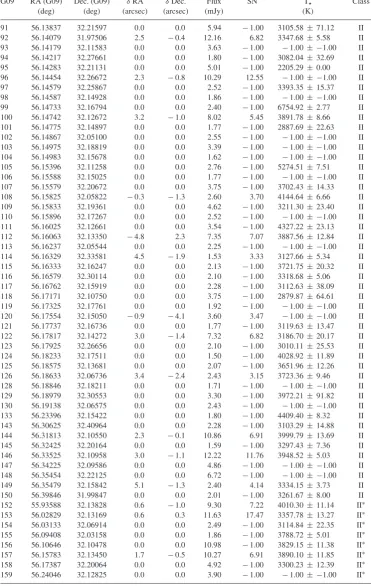
Table 2. IR excess matched sources. Entries with−1 indicate that we have no detections. Sources 49, 59, and 70 potentially contain flux from nearby cloud material. We mark these fluxes with a ‘’ and treat them as upper limits in the statistical analysis below. Class I∗sources, following the nomenclature of Gutermuth et al. (2009), are ‘deeply embedded’ Class I sources. IR excess matched sources. Class II∗sources, following the nomenclature of Gutermuth et al. (2009), are transition disc (TD) candidates.

G09 RA (G09) Dec. (G09) δRA δDec. Flux SN T Class

(deg) (deg) (arcsec) (arcsec) (mJy) (K)

4 56.10358 32.23000 0.0 0.0 2.76 −1.00 −1.00± −1.00 I∗

12 56.03833 32.04381 2.6 3.5 9.22 8.06 4106.23±58.13 I

14 56.12625 32.19314 0.0 0.0 3.18 −1.00 −1.00± −1.00 I

16 56.30758 32.20278 5.0 −2.5 7.51 10.31 −1.00± −1.00 I

18 55.84813 32.20719 0.0 0.0 2.16 −1.00 3087.79±12.62 II

19 55.86750 32.03311 0.0 0.0 1.95 −1.00 3789.68±4.84 II

23 55.94850 32.15072 0.0 0.0 5.79 −1.00 2654.35±45.64 II

24 55.95342 32.26433 0.0 0.0 1.80 −1.00 3464.19±5.74 II

26 55.98029 32.13147 0.0 0.0 1.50 −1.00 2711.48±31.18 II

30 55.98492 32.16647 0.0 0.0 4.59 −1.00 2139.14±0.55 II

32 55.99404 32.29100 −0.1 −1.7 3.41 4.44 3369.24±4.43 II

33 55.99546 32.19086 1.4 −1.6 2.01 3.44 3701.93±4.88 II

34 55.99617 32.23928 1.8 0.2 3.66 5.30 3156.47±28.06 II

41 56.02500 32.25894 0.0 0.0 6.93 −1.00 2682.95±29.85 II

43 56.04221 32.06792 0.0 0.0 1.98 −1.00 2868.23±17.81 II

45 56.04792 32.30264 0.0 0.0 4.26 −1.00 −1.00± −1.00 II

46 56.04842 32.05364 0.0 0.0 2.88 −1.00 6140.89±26.31 II

47 56.05408 32.22097 0.0 0.0 8.37 −1.00 2937.47±18.88 II

48 56.06346 32.32842 0.0 0.0 1.41 −1.00 −1.00± −1.00 II

49 56.06600 31.99356 −1.2 0.0 4.24 _{6.04 2842.07±21.67 II}

50 56.07537 32.18153 0.0 0.0 3.57 −1.00 4067.21±50.96 II

51 56.07571 32.08253 3.1 −0.9 31.20 10.28 5318.05±28.09 II

52 56.07579 32.16647 0.0 0.0 2.40 −1.00 3204.55±22.33 II

53 56.07746 32.21478 1.4 0.4 2.87 3.24 2652.84±79.92 II

54 56.08017 32.12628 0.0 0.0 4.17 −1.00 3516.26±16.30 II

55 56.08408 32.14906 0.0 0.0 2.25 −1.00 3351.63±10.00 II

56 56.08842 32.02067 0.0 0.0 2.58 −1.00 −1.00± −1.00 II

57 56.08867 32.21033 0.0 0.0 2.04 −1.00 3046.85±27.42 II

58 56.08871 32.19900 0.0 0.0 2.58 −1.00 3716.55±10.36 II

59 56.08896 31.99239 −3.8 −2.2 13.46 _{11.26 1529.32±1.48 II}

60 56.09008 32.17714 0.0 0.0 3.45 −1.00 3901.05±11.28 II

62 56.09287 32.09522 0.0 0.0 5.10 −1.00 4079.71±12.32 II

63 56.09300 32.20019 0.0 0.0 2.55 −1.00 3701.25±24.66 II

64 56.09458 32.02842 0.0 0.0 1.86 −1.00 −1.00± −1.00 II

65 56.09558 32.24461 0.0 0.0 2.88 −1.00 −1.00± −1.00 II

66 56.09821 32.15939 0.0 0.0 3.39 −1.00 2906.62±26.26 II

67 56.09850 32.03131 0.0 0.0 1.89 −1.00 −1.00± −1.00 II

68 56.10192 32.02883 0.0 0.0 1.98 −1.00 −1.00± −1.00 II

69 56.10542 32.17022 0.0 0.0 2.55 −1.00 3051.45±16.40 II

70 56.10637 32.19194 −1.5 0.6 6.44 _{3.93 3865.53±25.97 II}

71 56.10708 32.26369 0.0 0.0 4.44 −1.00 −1.00± −1.00 II

72 56.10846 32.07508 0.0 0.0 2.46 −1.00 4680.76±13.35 II

73 56.11121 32.13897 4.0 1.0 4.74 3.40 3782.54±11.35 II

74 56.11112 32.04342 0.0 0.0 2.94 −1.00 −1.00± −1.00 II

75 56.11337 32.34133 0.0 0.0 1.47 −1.00 2955.00±10.36 II

76 56.11354 32.17703 0.0 0.0 2.91 −1.00 2986.15±33.23 II

77 56.11354 32.23917 0.0 0.0 1.95 −1.00 3375.08±5.81 II

78 56.11879 31.99831 0.0 0.0 3.84 −1.00 3537.16±7.41 II

79 56.12062 32.02717 −2.9 2.2 3.77 3.96 3594.34±38.74 II

80 56.12179 32.02106 0.0 0.0 2.67 −1.00 −1.00± −1.00 II

81 56.12387 32.17775 0.0 0.0 2.70 −1.00 4045.34±11.51 II

82 56.12425 32.01517 0.0 0.0 2.49 −1.00 2735.18±20.87 II

83 56.12488 32.16097 0.0 0.0 3.30 −1.00 −1.00± −1.00 II

84 56.12554 32.02172 0.0 0.0 2.70 −1.00 3690.22±40.69 II

85 56.12896 32.04561 0.0 0.0 4.71 −1.00 3044.82±162.39 II

86 56.12975 32.31347 0.0 0.0 5.34 −1.00 −1.00± −1.00 II

87 56.12996 32.09972 −3.5 −0.0 6.80 3.08 3344.95±143.18 II

88 56.13062 32.17972 0.0 0.0 2.31 −1.00 3301.95±15.83 II

89 56.13071 32.00389 0.0 0.0 3.06 −1.00 3794.67±19.18 II

90 56.13488 32.05761 0.0 0.0 3.51 −1.00 −1.00± −1.00 II

Table 2 –continued

G09 RA (G09) Dec. (G09) δRA δDec. Flux SN T Class

(deg) (deg) (arcsec) (arcsec) (mJy) (K)

91 56.13837 32.21597 0.0 0.0 5.94 −1.00 3105.58±71.12 II

92 56.14079 31.97506 2.5 −0.4 12.16 6.82 3347.68±5.58 II

93 56.14179 32.11583 0.0 0.0 3.63 −1.00 −1.00± −1.00 II

94 56.14217 32.27661 0.0 0.0 1.80 −1.00 3082.04±32.69 II

95 56.14283 32.21131 0.0 0.0 5.01 −1.00 2205.29±0.00 II

96 56.14454 32.26672 2.3 −0.8 10.29 12.55 −1.00± −1.00 II

97 56.14579 32.25867 0.0 0.0 2.52 −1.00 3393.35±15.37 II

98 56.14587 32.14928 0.0 0.0 1.86 −1.00 −1.00± −1.00 II

99 56.14733 32.16794 0.0 0.0 2.40 −1.00 6754.92±2.77 II

100 56.14742 32.12672 3.2 −1.0 8.02 5.45 3891.78±8.66 II

101 56.14775 32.14897 0.0 0.0 1.77 −1.00 2887.69±22.63 II

102 56.14867 32.05100 0.0 0.0 2.55 −1.00 −1.00± −1.00 II

103 56.14975 32.18819 0.0 0.0 3.39 −1.00 −1.00± −1.00 II

104 56.14983 32.15678 0.0 0.0 1.62 −1.00 −1.00± −1.00 II

105 56.15396 32.11258 0.0 0.0 2.76 −1.00 5274.51±7.51 II

106 56.15588 32.15025 0.0 0.0 1.77 −1.00 −1.00± −1.00 II

107 56.15579 32.20672 0.0 0.0 3.75 −1.00 3702.43±14.33 II

108 56.15825 32.05822 −0.3 −1.3 2.60 3.70 4144.64±6.66 II

109 56.15833 32.19361 0.0 0.0 4.62 −1.00 3211.30±23.40 II

110 56.15896 32.17267 0.0 0.0 2.52 −1.00 −1.00± −1.00 II

111 56.16025 32.12661 0.0 0.0 3.54 −1.00 4327.22±23.13 II

112 56.16063 32.13350 −4.8 2.3 7.35 7.07 3887.56±12.84 II

113 56.16237 32.05544 0.0 0.0 2.25 −1.00 −1.00± −1.00 II

114 56.16329 32.33581 4.5 −1.9 1.53 3.33 3127.66±5.34 II

115 56.16333 32.16247 0.0 0.0 2.13 −1.00 3721.75±20.32 II

116 56.16579 32.30114 0.0 0.0 2.10 −1.00 3318.68±5.06 II

117 56.16762 32.15919 0.0 0.0 2.28 −1.00 3112.63±38.09 II

118 56.17171 32.10750 0.0 0.0 3.75 −1.00 2879.87±64.61 II

119 56.17325 32.17761 0.0 0.0 1.92 −1.00 −1.00± −1.00 II

120 56.17554 32.15050 −0.9 −4.1 3.60 3.47 −1.00± −1.00 II

121 56.17737 32.16736 0.0 0.0 1.77 −1.00 3119.63±13.47 II

122 56.17817 32.14272 3.0 −1.4 7.32 6.82 3186.70±20.17 II

123 56.17925 32.26656 0.0 0.0 2.10 −1.00 3010.11±25.53 II

124 56.18233 32.17511 0.0 0.0 1.50 −1.00 4028.92±11.89 II

125 56.18575 32.13681 0.0 0.0 2.07 −1.00 3651.96±12.26 II

126 56.18633 32.06736 3.4 −2.4 2.43 3.15 3723.36±9.46 II

128 56.18846 32.18211 0.0 0.0 1.71 −1.00 −1.00± −1.00 II

129 56.18979 32.30553 0.0 0.0 3.30 −1.00 3972.21±91.82 II

130 56.19138 32.06575 0.0 0.0 2.43 −1.00 −1.00± −1.00 II

133 56.23396 32.15422 0.0 0.0 1.80 −1.00 4409.40±8.32 II

143 56.30625 32.40964 0.0 0.0 2.28 −1.00 3103.29±14.88 II

144 56.31813 32.10550 2.3 −0.1 10.86 6.91 3999.79±13.69 II

145 56.32425 32.20164 0.0 0.0 1.59 −1.00 3297.43±7.36 II

146 56.33525 32.10958 3.0 −1.1 12.22 11.76 3948.52±5.03 II

147 56.34225 32.09586 0.0 0.0 4.86 −1.00 −1.00± −1.00 II

148 56.35454 32.22125 0.0 0.0 6.72 −1.00 −1.00± −1.00 II

149 56.35479 32.15842 5.1 −1.3 2.40 4.14 3334.15±3.73 II

150 56.39846 31.99847 0.0 0.0 2.01 −1.00 3261.67±8.00 II

152 55.93588 32.13828 0.6 −1.0 9.30 7.22 4010.30±11.14 II∗

153 56.02829 32.13169 0.6 0.3 11.63 17.47 3357.78±13.27 II∗

154 56.03133 32.06914 0.0 0.0 2.49 −1.00 3114.84±22.35 II∗

155 56.09408 32.03158 0.0 0.0 1.86 −1.00 3788.72±5.01 II∗

156 56.10646 32.10478 0.0 0.0 10.98 −1.00 3829.15±11.38 II∗

157 56.15783 32.13450 1.7 −0.5 10.27 6.91 3890.10±11.85 II∗

158 56.17387 32.20064 0.0 0.0 4.92 −1.00 3300.23±12.39 II∗

159 56.24046 32.12825 0.0 0.0 3.90 −1.00 −1.00± −1.00 II∗

2.3.2 Literature mm detections

Recently, Ru´ız-Rodr´ıguez et al. (2018) published an ALMA study

of the discs in the IC 348 region, undertaken at 1.3 mm. This study performed a snapshot survey of 136 sources classified as Class II

objects by Lada et al. (2006) and Muench et al. (2007), detecting

40 with a 3σsensitivity of∼0.45 mJy at 1.3 mm. This noise limit is

roughly two times lower than the best noise floor the LMT achieves at 1.1 mm in this study; however, as we discuss below in Section 3.3, the expected scaling of the flux with wavelength makes the LMT

Table 3. Table of LMT data sources (cf. Table 2) matched to the source list of Gutermuth et al. (2009).

Designation Number

LMT+Gutermuth et al. (2009)

Matches 116

Detections 28

Upper limits 88

Ru´ız-Rodr´ıguez et al. (2018)+Gutermuth et al. (2009)

Matches 116

Detections 40

Upper limits 76

Cottaar et al. (2014)+Gutermuth et al. (2009)

Matches 100

LMT detections 24

LMT upper limits 61

Matches not covered by LMT 15

competitive in placing physical constraints on the systems. Of the

136 sources classified as Class II objects by Lada et al. (2006)

and Muench et al. (2007), 20 are not classified as Class II objects

in the catalogue of Gutermuth et al. (2009).1_{We exclude the 20}

sources from Lada et al. (2006) and Muench et al. (2007) that are

not included in Gutermuth et al. (2009) from our analysis of Class

II sources.

Additional previous studies have targeted IC 348 at mm

wave-lengths. Lee et al. (2011) surveyed 85 sources in IC 348 with

the Submillimeter Array (SMA) at 1.3 mm (230.5 GHz) and detected 10 sources with fluxes greater than 2 mJy. Espaillat et al.

(2012) observed five sources in IC 348 with the SMA at 0.86 mm

(345 GHz), obtaining two detections with fluxes greater than 15

mJy. Cieza et al. (2015) detected 13 sources at 850μm with fluxes

greater than 5 mJy. Owing to the small sample sizes of these studies

(particularly compared to Ru´ız-Rodr´ıguez et al. 2018) and the

uncertainty relating to translating fluxes between wavelengths (see Section 3.3), we opt to use only the observations of Ru´ız-Rodr´ıguez

et al. (2018) in our analysis.

2.3.3 Stellar properties

For stellar characterization, we use previous studies to determine spectral type, effective temperature, bolometric luminosity, and mass of the stars hosting circumstellar discs. IC 348 was observed by the ancillary program INfrared Spectra of Young Nebulous

Clusters (IN-SYNC; Cottaar et al.2014), part of the Apache Point

Observatory Galactic Evolution Experiment (APOGEE; Zasowski

et al.2013; from the third Sloan Digital Sky Survey, Eisenstein et al.

2011). IN-SYNC uses a multi-object, high-resolution (R∼22 500)

spectrograph with a spectral coverage from 1.51 to 1.69μm. In

Cottaar et al. (2014), stellar parameters are derived by matchingH

-band spectra to a grid of synthetic spectra using aχ2_minimization

technique and Monte Carlo Markov Chain technique to estimate errors. The fits have five parameters: effective temperature, surface

gravity, radial velocity, rotational velocity, and H-band veiling

1_{The unified list of Class II objects between Lada et al. (2006), Muench} et al. (2007), and Gutermuth et al. (2009) has 116 members, coincidentally the same number of sources we observed from the Gutermuth et al. (2009) sample alone.

(to account for emission from a hot inner circumstellar disc). Allowing physical parameters to vary allows for a more robust characterization of the stellar source than mapping spectral types to temperatures, particularly for young objects (see Bary & Petersen

2014for an example).

The source list of Gutermuth et al. (2009) was matched to the

source list of IN-SYNC (Cottaar et al. 2014) at a tolerance of

1.0 arcsec, returning 100 matches. The remaining 60 sources from

Gutermuth et al. (2009) were not observed, principally owing to

the limit magnitude of IN-SYNC inH-band (typicallyH<12.5).

The list of 100 matched sources was matched with a maximum radial tolerance of 5 arcsec to the flux-weighted centroid from the

LMT source list. The middle frame of Table3lists the summarized

matching numbers between the Gutermuth et al. (2009) and

IN-SYNC, with additional unification with the LMT-measured sources. In principle, it is possible to use the same BT-SETTL model

isochrones (Allard, Homeier & Freytag 2011) as IN-SYNC to

determine the luminosity, mass, and age of stellar sources. The luminosity, mass, and age are determined by a simple one-to-one mapping to temperature and surface gravity similar to the procedure

used in Andrews et al. (2013); we interpolate a grid of effective

temperature and surface gravity from the BT-SETTL models to determine luminosity, mass, and age of stellar sources. However, owing to the uncertainties that are introduced by the models, we choose to restrict ourselves to the published stellar parameter values and do not include the uncharacterized 60 sources in our discussion regarding the relationship of stellar parameters and disc flux.

Additionally, using IN-SYNC data, Fernandez et al. (2017) found

two of the disc-bearing sources from Gutermuth et al. (2009) to be

binaries (Sources 116 and 158, using the identification of Gutermuth

et al.2009and Table2). Both were covered by our sample, but were

not detected. Upper limits of 2.1 and 4.92 mJy were measured, respectively.

2.4 Source matching

We use the source list of Gutermuth et al. (2009) as the master list

of YSOs in IC 348, a total of 160 sources. In Table3, we summarize

the matching number of sources between Gutermuth et al. (2009),

the LMT detections from this study (discussed in Section 2.2), the

stellar properties of Cottaar et al. (2014), and the ALMA study of

Ru´ız-Rodr´ıguez et al. (2018). The middle frame of Table3lists

the summarized matching numbers between the Gutermuth et al.

(2009) and Ru´ız-Rodr´ıguez et al. (2018).

There are 141 YSOs (139 from Gutermuth et al.2009, with two

additional candidates discussed below in Section 3.2) that lie within the ALMA and LMT footprints, with each telescope covering 116 sources (source overlap means that the samples are not distinct, despite both samples coincidentally having 116 sources from the

list of Gutermuth et al.2009). Of those sources covered, the LMT

detects 28 and ALMA detects 40, with 24 sources in common between the two samples. As a result, we have 44 sources with mm-flux measurements from one of the two programs; choosing the more stringent upper limit measurement for the remainder results in a sample of 97 upper limits, with 74 from ALMA and 23 from LMT. When the more stringent limit is chosen, the LMT provides coverage of 51 sources, while ALMA provides coverage of 90

sources. The comparison is summarized in Table4.

Additionally, we queriedGaiaData Release 2 (Gaia

Collabora-tion2016,2018) in a 30 arcmin radius circle for Class II sources

in IC 348, as determined by Gutermuth et al. (2009). Using a

matching tolerance of 1 arcsec, we find 127 of the 160 sources to

Table 4. Table of ALMA sources matched to the LMT photometry. We exclude the 20 ALMA targets that are not infrared excess sources from Gutermuth et al. (2009) for this matching. We also exclude two candidate TDs that do not appear in the Gutermuth et al. (2009) list for this matching.

Designation Number covered

Total Gutermuth et al. (2009) coverage (LMT–ALMA union) 139

Total LMT–ALMA overlap (LMT–ALMA intersection) 93

Overlapping detections 24

LMT limits, ALMA detections 11

ALMA limits, LMT detections 2

ALMA limits, deeper than LMT limits 56

LMT detections, no ALMA coverage 2

ALMA detections, no LMT coverage 16

ALMA limits, no LMT coverage 5

LMT limits, no ALMA coverage 23

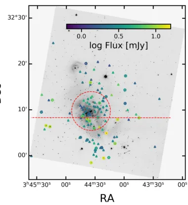
Figure 2. IRAC Channel 2 (4.5μm) greyscale image of the IC 348 region. The spatial distribution of YSOs measured as part of the survey, drawn from the sample of Gutermuth et al. (2009) is overlaid, with circle symbols representing discs from the LMT sample, and triangles representing upper limits. The symbols are colour-coded to correspond to the flux in mJy. Two partitions, separating the equal populations, are shown. An inner/exterior partition based on the central B5 binary is shown as a red dashed circle. A north/south partition (red dashed line) is also shown.

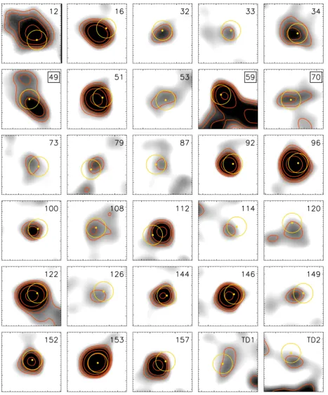
Figure 3. Inverse greyscale cropped LMT/AzTEC 1.1mm images of the 30 arcsec×30 arcsec surrounding IC 348 members detected at 1.1mm. The numbers in the upper right corner of each panel correspond to the Gutermuth et al. (2009) identifiers, as in Table2. The panels labelled ‘TD1’ and ‘TD2’ correspond to the candidate TDs, as in Table5. The greyscale stretch is linear, with white to black spanning from−1 to 5 times the median noise value for each field of view. The red contours mark S/N=2.5, 3.5, 4.5, 6.5, 10.5, 18.5. The gold plot points mark the location of each matched YSO, and the surrounding circle shows the 5 arcsec matching radius. Objects 49, 59, and 70 are marked to draw attention to their substantial confusion with adjacent cloud material, and are treated as upper limits in our statistical analysis.

Ta b le 5 . Candidate ne w T Ds. T he photometry is tak en from G utermuth et al. ( 2009 ). Inde x 2 MASS RA Dec. δ RA δ Dec. T (de g ) (de g) (arcsec) (arcsec) (K) TD1 J03444016 + 3209129 56.16734 32.15358 3.2 − 0.8 3084.11 ± 18.30 TD2 J03443588 + 3215028 56.14952 32.25079 1.8 4 .5 4038.99 ± 19.13 Inde x J H K 3.6 μ m4 .5 μ m5 .8 μ m8 .0 μ m2 4 μ m 1 .1 mm Flux 1.1 m m S N (mag) (mag) (mag) (mag) (mag) (mag) (mag) (mag) (mJy) TD1 13.34 ± 0.02 12.23 ± 0.02 11.74 ± 0.02 11.23 ± 0.02 11.11 ± 0.03 − 1. − 1. > 3.6 3 .69 3 .38 TD2 12.84 ± 0.02 11.56 ± 0.02 11.09 ± 0.02 10.78 ± 0.01 10.69 ± 0.01 10.55 ± 0.01 10.63 ± 0.04 > 6.9 5 .39 3 .47

have reliable matches. Of the 127 sources, 99 sources have parallax

measurements, with a median distance of 322.6 ± 28.5 pc. We

therefore adopt 320 pc value as the distance to the cluster, in line with previous estimates and other works. Of the 20 sources observed

in Ru´ız-Rodr´ıguez et al. (2018) that do not appear in the IR excess

list of Gutermuth et al. (2009), seven are present inGaiaDR2, and

are all consistent with being at the distance of IC 348 (within 2σof

320 pc).

3 R E S U LT S

In this section, we first present the measurements from our LMT survey in Section 3.1. Section 3.2 reports two new candidate TDs serendipitously identified in our fields. In Section 3.3, we combine

our results with that of Ru´ız-Rodr´ıguez et al. (2018) to make a

master list of disc detections in IC 348, described in Section 3.4.

3.1 LMT measurements at 1.1 mm

Table2lists the LMT data for 116 sources from Gutermuth et al.

(2009), and Fig.3shows those YSOs with associated LMT/AzTEC

detections. In Fig.2, we plot the measured 1.1 mm fluxes as

colour-coded symbols on top of the IRAC Channel 2. Detected sources are shown as circles, while upper limits are squares. As listed in

Table3, we detect 28 sources from the list of Gutermuth et al. (2009),

with 88 additional upper limits. We detect 2

4=0.5 of the Class I

objects covered, and₁₁₂26 =0.232 of known Class II objects covered

(including TDs). For later analysis (Section 4.1), we show two

methods with which to partition the data in Fig.2, based on the most

massive system of IC 348, the B5 binary HD 281159: a north/south cut on the declination of the B5 system, and an interior/exterior cut based on a 5 arcmin radius projection drawn from the B5 system. Both samples are divided such that the number of objects in each partition is equal.

As has been used extensively in the literature, a disc mass can be crudely estimated from a simple scaling of the mm-wave continuum

luminosity (Hildebrand1983; Beckwith et al.1990). Assuming the

emitting dust is optically thin and isothermal, the dust mass may be described as

Md=

Fν·d2

ζ·κν·Bν

, (1)

whereκνis dust opacity,ζis the dust-to-gas mass ratio,dis distance,

andBν(Td) is the Planck function at the average disc temperature.

Following Andrews & Williams (2005) and Andrews et al. (2013),

we use ζ = 0.01,κν = 2.3 cm2g−1. The uncertainty inζ and

κν is likely to dominate, with errors up to an order of magnitude

possible. We take 1.1 mm to be the reference wavelength, and

follow the standard assumption in Andrews & Williams (2005) that

Td 20 K is applicable for all discs, though we acknowledge that

this assumption is also highly uncertain. Andrews et al. (2013) did

use a relationship for host star luminosity and dust temperature,

Td = 25(L/L)1/4 K derived from a radiative transfer analysis

including a disc which is not completely optically thin (such that there is an inner heating contribution), but owing to the small temperature range of the host stars in our sample (the majority

satisfy 3.4<logTeff<3.8) and the shallow slope of the relation,

the dust temperature difference is trivial. As it is highly uncertain

whether in the relationship between mm flux andMdis a simple

linear scaling, for lack of a clear answer, we will assume for our analysis that the mm flux scales monotonically with the dust mass in the disc, such that discs with higher flux are more massive.

Further, mass determinations from models such as Espaillat

et al. (2011) are consistently higher than Andrews & Williams

(2005). The opacities used are approximately three times lower

and the models use a larger outer disc radius and self-consistent surface density and temperature instead of power-law approxima-tions. Therefore, masses obtained by different models cannot be meaningfully compared. We reserve the modelling of disc SEDs for future work, particularly when the dust emissivity may be more precisely constrained.

For posterity, under the standard assumptions discussed above,

we report thatF1.1 mm = 6.94 M⊕/mJy, but do not use the disc

masses in our analysis, noting instead that the disc mass under these assumptions is directly proportional to flux, and instead choose to perform our analysis on flux only.

As we discuss below, our data suggest a different spectrum for dust opacity, which translates into a different flux-to-mass conver-sion. Dust opacity in circumstellar discs is discussed extensively in

Andrews & Williams (2007), and we follow their equation (3) to

provide a possible scalingκν from 1.3 mm (225 GHz) to 1.1 mm

(265.9 GHz)

κν =κ0

ν ν0

β

=3.55. (2)

Comparing with the typically assumedβvalue, our impliedβwill

result in a factor of 1.55 change for the conversion of flux to mass.

Therefore, a scaling of flux to mass withF1.1mm=4.5 Mearth/mJy is

also allowed by our data. As we will consistently refer to flux only throughout the paper, this range of mass conversions does not affect our results.

3.2 New candidate transition discs discovered via mm-wave photometry

The mm survey reported here targeted a list of known infrared

excess sources from Gutermuth et al. (2009), including the 10

known TDs in IC 348. In addition, two known members of IC 348

(Cottaar et al.2014) that were considered discless based on Spitzer

IR observations were detected serendipitously in our mm maps,

although at low S/N (see Fig.3). We propose that these may be

TDs with massive, cold outer discs and substantial inner gaps. Statistical comparisons to the more numerous lists of field stars in the Spitzer IR catalogue show that the small matching tolerance (5 arcsec) afforded by the excellent astrometry of the LMT means that the mm detections have a vanishingly small likelihood of being accidental matches to coincident IC 348 members.

Neither of the two newly identified candidate TDs was detected in

Spitzer/MIPS 24μm coverage. To estimate the 24μm upper limits

from the data, we computed a new, spatially resolved (30 arcsec), 90 per cent differential completeness map for the Gutermuth et al.

(2009) MIPS source extraction, using the method of Gutermuth &

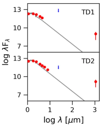
Heyer (2015). We plot the SEDs of the two candidates in Fig.4,

with the local 24μm completeness limits for each source shown

in blue to demonstrate that the 24μm constraints cannot rule out

excess emission. The objects appear to have strong mm emission consistent with a cold circumstellar disc. If further observations confirm their nature as TDs, it is suggestive that sensitive mm-wave continuum mapping of nearby star-forming regions, with facilities such as LMT and the new TolTEC continuum array camera (Bryan

et al.2018), are likely to discover more such inner-gap discs among

stars where MIPS 24μm photometry simply could not constrain

sufficiently to ensure that no disc is present.

Figure 4. Spectral energy distributions of two candidate TDs. The grey spectra are an M5 (upper panel) and K7 (lower panel) from the spectral library of Rayner, Cushing & Vacca (2009), extrapolated using a Rayleigh– Jeans approximation beyond 5μm. The choice of comparison spectrum corresponds to the effective temperature measured from IN-SYNC data. For both, the measured 24μm point is an upper limit (shown in blue). Owing to the non-constraining nature of these limits, combined with the lack of significant excess emission in the mid-infrared, the sources were classified as discless by Gutermuth et al. (2009).

The possibility that still-undiscovered TDs lurk in nearby star-forming regions sheds new light on the apparent disagreement between IC 348 and other young clusters put forth in Muzerolle

et al. (2010), which found that 12 per cent of the discs in IC 348 are

TDs. Additionally, the discovery of new TDs via a deep mm search provides an interesting avenue for identifying systems where planets may be forming. As we cannot be certain that our sample is complete to unidentified TDs, we do not place a constraint on the fraction of TDs, but rather advocate for a survey that includes all known

members whose MIPS 24 μm flux cannot rule out the presence

of a TD. Further, other regions may benefit from blind searches, particularly as new facilities that can perform such obervations come online.

3.3 Connection with ALMA

Given the opportunity to compare data sets, we wish to examine our results as compared to those of ALMA to characterize the

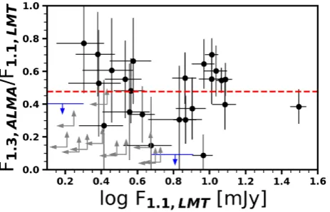
sources. Fig.5plots LMT and ALMA fluxes for matched sources

(i.e. the 24 mutual detections). We additionally show 11 sources with ALMA detections but no LMT detection (grey arrows), as well as two sources with LMT detections and no ALMA detection (blue arrows). With the 24 overlapping sources, the mean of the ratio for detected sources is 0.476 (unweighted) and 0.461 (flux weighted), as indicated by the dashed line.

The conversion of data points to different wavelengths relies on

the relationshipFν ∝να, whereα=β+2.β, the dust emissivity,

Figure 5. Ratio of ALMA 1.3 mm fluxes to LMT 1.1 mm fluxes as a function of LMT fluxes for 24 matched sources. The black points have detections in both the ALMA and LMT surveys. The grey arrows have detections in ALMA but upper limits in the LMT data, and are thus lower limits. The blue arrows have detections in the LMT data but no detection in ALMA, and are therefore upper limits.

is related to the flux ratio by

β= log (F1.3mm/F1.1mm)

log (1.1/1.3) −2

= −13.7 log

F1.3mm F1.1mm

−2. (3)

The dust emissivity is related to the dust opacity asκν = Cνβ,

whereCis some constant. The theoretically expected value at long

wavelengths, via the Kramers–Kroenig relations (Purcell1969), is

β=2.

Assuming 15 per cent uncertainty in each mean flux,2_the

uncer-tainty in the mean flux ratio is∼21 per cent, and thus the uncertainty

in the logarithm of the ratio is 0.09. Our flux-weighted finding of F1.3mm/F1.1mm=0.461 propagates toβ=2.61±1.24. As we report

a 1σ error bar, we have no strong constraint on β here, but we

are consistent with theoretical predictions. Unfortunately, we are severely limited by the independent calibration uncertainties and the narrow wavelength difference. However, in the Taurus region,

Andrews et al. (2013) foundα=2.4±0.5, which is equivalent to

β=0.4, a stark departure from what we calculate here, although

both measurements are statistically consistent owing to their large

uncertainties. The strongly different values of β again caution

against simple scaling of mm flux to disc mass. The uncertainty in the LMT photometry makes drawing detailed conclusions about the SED slope difficult at present for individual sources, but future in-struments will be able to provide more information. Throughout the

rest of the work, we will use the relationshipF1.1 mm=2.12F1.3 mm

to transform IC 348 data from Ru´ız-Rodr´ıguez et al. (2018), as

calibrated above.

3.4 Merged disc list

We use the infrared excess list of Gutermuth et al. (2009) as our

guide to create a master list of disc measurements in IC 348. Of

the 136 sources reported in Ru´ız-Rodr´ıguez et al. (2018), 20 do not

appear on the list in Gutermuth et al. (2009), indicating that they

2_{We have an error of a few per cent on the individual fluxes, but we} acknowledge a likely 10 per cent overall calibration uncertainty.

may have been misclassified as disc-bearing objects in previous

studies (Lada et al.2006; Muench et al.2007). For the purposes

of our research here, we exclude those sources from the candidate disc sample. Doing so does not exclude any of the detections from

Ru´ız-Rodr´ıguez et al. (2018), only upper limits. As none of the 20

sources in the sample of Ru´ız-Rodr´ıguez et al. (2018) without a

match in the Gutermuth et al. (2009) catalogue have detections, we

interpret this as supporting evidence that the sources were likely misclassified.

As discussed in Section 2.4 and summarized in Table 4, we

compile a unified source list which covers 139/160 infrared excess

sources identified in Gutermuth et al. (2009), including 93/139 with

temperature measurements from IN-SYNC (Cottaar et al.2014).

With the addition of the two candidate TDs, we create a master list of mm flux measurements for 141 sources with infrared (or potential infrared) excess. We choose to compile the fluxes at 1.1 mm. Therefore, we prioritize LMT detections in cases with

overlap (the 28 LMT-detected sources, cf. Table3) as the primary

detections, supplementing with 16 ALMA scaled detections. For limits, we first scale the ALMA measured upper limits, then select the more stringent limit in cases of overlap. This sample is analysed in Section 4.1. Comparing this net sample to IN-SYNC, we find that 25/28 LMT detections have stellar parameters, as well as 12/16 ALMA detections. 11/23 LMT upper limits and 46/74 ALMA upper limits have stellar parameters. Summing the numbers, 94/141 sources have stellar parameters. The cross-matched sample is used in Sections 4.2 and 4.3.

Unfortunately, owing to the incomplete nature of the observations

of the Class II sample from Gutermuth et al. (2009), as well as

the possible presence of previously unknown TDs, we can only place a loose constraint on the 1.1 mm disc mass fraction with f1.1 mm>1mJy:fd,>1 mJy= ₁₄₁44 =0.31+₋00..0904. The upper (lower) limit

is calculated assuming all 21 sources in the Class II sample of

Gutermuth et al. (2009) for which we do not have coverage are

measured to have fluxes above (below) 1 mJy.3 _{This is similar}

to the number reported in Ru´ız-Rodr´ıguez et al. (2018):fd,>1 mJy=

40

116 =0.34, when only counting sources defined by Gutermuth et al.

(2009).

4 A N A LY S I S

In this section, we first present the luminosity function of the detected discs in IC 348 in Section 4.1. We present basic analysis of the millimetre measurements as related to additional information on the stellar hosts (Section 4.2), including rotation rates (Section 4.3).

4.1 Cumulative luminosity function

Examining Fig.2, we do not see any obvious spatial correlations

with our detections, including a lack of correlation with the infrared nebulosity. However, the lower half of the cluster contains almost

all of the bright detections (logFmm > 0.6), consistent with a

south-to-north age gradient in the cluster. Additionally, the centre of the cluster, within 5 arcmin of the central B5 binary, appears to have a dearth of disc detections. In this section, we will use a product-limit estimator formalism and cumulative luminosity functions to show that the north/south populations are distinct at

3_{If we were to include the 20 potentially misclassified sources observed in} the sample of Ru´ız-Rodr´ıguez et al. (2018), the disc fraction would reduce tofd,>1 mJy=₁₆₁44 =0.27+₋0.090.03.

Figure 6. Cumulative flux distributions for IC 348. Left-hand panel shows subdivision of northern and southern halves, as indicated in2, right-hand panel shows subdivision of cluster interior (<5 arcmin from the central B5 binary) and cluster exterior, also indicated in2. The solid lines are for the LMT results only, transparent thick lines are for ALMA results only. ALMA sources have been scaled to be at 1.1 mm.

high significance, and that the interior/exterior populations are also distinct, albeit at a more modest significance. We interpret this as evidence for (1) asynchronous star formation across the cluster, and/or (2) environmental effects from the central B5 binary.

Fig. 6presents the cumulative 1.1 mm luminosity distribution

functions for IC 348, divided into north/south and interior/exterior partitions (left- and right-hand panels, respectively). The distribu-tions are made following the formalism for Kaplan–Meier product-limit estimator to properly account for censored measurements

(upper limits onFmm) as described in Feigelson & Nelson (1985).

In such a formalism, the high upper limits of some LMT sources can lead to a truncated distribution, owing to the uncertainty of the disc distribution function structure below the limit. Therefore, we also perform the same analysis on the ALMA results of

Ru´ız-Rodr´ıguez et al. (2018), finding indistinguishable curves, except for

the northern partition, which is missing three relatively high-flux

sources in Ru´ız-Rodr´ıguez et al. (2018).

The primary metric for comparing two censored samples used in

the literature is the Peto–Prentice test (Feigelson & Nelson1985).

The test returns p_∅, the probability that two samples are drawn

from the same parent distribution. As with many other statistical measures, the power of the metric lies in the ability to confidently say

that distributions arenotdrawn from a parent distribution. Unlike

previous mm disc detection works (e.g. Andrews et al.2013;

Ru´ız-Rodr´ıguez et al.2018), we do not construct a cumulative distribution

ofp∅, the so-called null hypothesis probability distributionf(<p∅).

The purpose in those works was to homogenize the sample of spectral types between different star-forming regions; in the case of IC 348, an examination of both the north/south and interior/exterior partitions does not show significant differences in the temperature distributions. Likewise, an examination of the spectral type distri-butions between the ALMA and LMT samples does not reveal any

significant differences (compare the range of temperatures in Fig.9).

Despite the apparent differences by eye in both panels of Fig.6,

the Peto–Prentice does not find strong evidence for differentiation between the two samples. The lack of sensitivity in the two-sample comparison is likely owing to the relatively small dynamic range of the detections. While the LMT north/south partition returns

p_∅ = 0.029, significant at the ∼2.5σ level, the same test on the

unified LMT–ALMA data set returns p∅ = 0.33, meaning the

samples are indistinguishable given this test.4_{The interior/exterior}

partitions place even less stringent constraints, withp_∅=0.21 for

the LMT only andp_∅=0.47 for combined sample.

However, we can use the Peto–Prentice formalism to investigate the importance of the choice of flux scaling that transforms the

ALMA points to the LMT reference wavelength:F1.1 mm=CF1.3 mm.

In Section 3.3, we calculated C= 2.12, but the α value of 2.4

derived by Andrews et al. (2013), using a sample of 60 sources in

Taurus with multiple detections between 0.7 and 3 mm, corresponds

to C = 1.49 ± 0.13. The Andrews et al. (2013) value for C

has been used throughout the literature to homogenize data sets across different wavelengths for comparison between clusters (e.g.

Ru´ız-Rodr´ıguez et al.2018). We test the validity ofCTaurusbeing

used for IC 348 by comparing the cumulative distribution functions between the LMT and scaled ALMA distributions for a range of

avalues. When we useC=2.12, we findp∅=0.59, well within

1σ, implying that the distributions cannot be distinguished. When

using theCTaurus=1.49, we findp∅=0.13, still within 2σ, and thus

indistinguishable. At the 3σ level, where it can be strongly stated

that the samples are not drawn from the same parent distribution,

we can excludeCIC 348 < 0.84 andCIC 348 > 18.25. While these

limits are not particularly constraining, asC<1 is aphysical, at the

2σ level, we can excludeCIC 348<1.18 andCIC 348>7.81. Fig.7

shows the distribution of logp_∅as a function ofC. A more complete,

deeper sample with multiple wavelength detections would be able to use this formalism to place more stringent limits.

In Fig.8, we perform two-sample tests on the divided IC 348

samples, as a function of the number of flux-sorted discs included. Our goal is to calculate the difference between the populations

of bright discs in the partitions. At each abscissa value x, we

calculate the two-sample null probability for the north/south and

interior/exterior population divisions. We select thexbrightest discs

from each sample and compare the probability the populations

4_{We assume the probabilities are drawn from aχ}2_{distribution, such that} p_∅ =0.317, 0.0455, 0.0027 correspond to the nominal 1σ, 2σ, and 3σ

probabilities.

Figure 7. Log null probability,p_∅, versusC, the scaling to convert between 1.1 and 1.3 mm fluxes:F1.1 mm=aF1.3 mm. The green horizontal lines denote 1σ, 2σ, and 3σvalues, from top to bottom. The grey vertical dashed line is a=2.12, the nominal value assumed in this work.

Figure 8. Log null probability,p_∅, as a function of flux-sorted disc samples. At each value ofndiscs, we perform a two-sample test on thenbrightest discs from each of the separated populations and plot the resulting value ofp_∅, for both the north/south (black) and interior/exterior partitions (red). The horizontal green bands correspond to 2σ(upper) and 3σ(lower).

were drawn from the same sample. As the populations have been divided in half, it is a fair comparison to choose the number of

discs rather than the fraction of discs. For ndiscs < 23 (19) in

the north/south (interior/exterior) divisions, we see strong evidence

(>3σ) for different populations. As the number of discs included

increases, the signal decreases. We interpret this as evidence for (a) a north–south gradient in star formation, and if we assume that the disc flux (mass) declines with time, the discs in the south are younger, and/or (b) disc photoevaporation from the central B5 binary that reduces the mass (flux) of the discs in the vicinity. In a disc photoevaporation scenario, we would be observing a loss of mass from the less bound portions of large-radius discs,

resulting in a truncation that preferentially affects the biggest discs

the most. Ansdell et al. (2017) found similar evidence in the form

of a dearth of discs around the OB stars inσOri. Future high spatial

resolution observations of discs in IC 348 are needed to test this hypothesis.

An alternative scenario is that the north–south gradient is ev-idence that the IC 348 region is inhomogeneous, and that the observations reflect the variation in density rather than age. Cottaar

et al. (2015) fit the distribution of IN-SYNC radial velocities with

one and two Gaussians, finding that the addition of a second Gaussian significantly improved the fit. The velocity dispersion is consistent with supervirial conditions, implying that the current evolution of the cluster is dominated by stellar and gas

mass-loss. Cottaar et al. (2015) propose a myriad of possibilities for the

observations, including that IC 348 is contaminated by the Perseus OB2 association, that IC 348 recently underwent a gas expulsion or merger event that created a dispersing halo of stars around IC 348, that IC 348 has not yet relaxed to a cluster with radial velocities that may be represented by a single Gaussian, and lastly that the region may be the superposition of two subclusters which are converging

along the line of sight. TheGaiadata presented by Ortiz-Le´on et al.

(2018) suggest based on proper motion analysis that a halo of stars

may be present around the cluster, but future data releases will be needed to fully characterize the region.

4.2 Dependences on stellar hosts

In Fig. 9, we plot surface temperature versus 1.1 mm flux for

all sources in the sample with IN-SYNC stellar parameters (see

Table4). The points are colour-coded with the IN-SYNC-derived

log (g) values. When not covered by the LMT, we use ALMA

observations for corresponding sources, scaled using a flux ratio ofF1.1 mm=2.12F1.3 mm. Overlapping sources between ALMA and

the LMT are shown using the LMT points if detected, or as the

more stringent limit in the case of upper limits (cf. Table3). The

addition of the ALMA detections, scaled as described in Section 3.3 to match the wavelength of the LMT, do not change the conclusions drawn from the LMT data alone, but provide valuable additional data.

To further demonstrate the strong difference between northern and southern partitions of IC 348, we divide the sources into those in the northern partition (left) and southern partition (right). While other regions such as Taurus (complete at temperatures hotter than

M8.5 Andrews et al.2013) exhibit a relationship (see discussion

below in Section 5.2), we do not find evidence for a conclusive relationship between stellar surface temperature and 1.1 mm flux. One possible explanation for the lack of relationship comes from

Cottaar et al. (2014), who also demonstrated a spread in intrinsic

stellar radii, indicative of an age spread where younger stars have had less time to contract towards the main sequence. Using similar

methodology where log (g) is an age indicator, Yao et al. (2018)

also found weak evidence for intra-cluster age variation. Our interpretation of differing star formation histories in the north and

south partitions supports the explanation of Cottaar et al. (2014)

and Yao et al. (2018).

We do not detect emission from two cool stars (Teff∼2000 K)

identified by Cottaar et al. (2014). The upper limits are reported in

Table2. Measurements of mm flux around very cool sources may

not be uncommon; Ward-Duong et al. (2018) measured 885μm

flux densities for 24 Taurus sources with late M spectral types,

and Ru´ız-Rodr´ıguez et al. (2018) detect mm emission from a