MODEL SELECTION AND BAYES ESTIMATES OF THE PARAMETER FOR
DISTRIBUTION OF WAITING TIME TO FIRST BIRTH
Sanjay Kumar Singh
*Department of Statistics and DST **Department of Community Medicine and DST
ARTICLE INFO ABSTRACT
This paper considers various models for first birth interval to a married woman with an aim to pick up a model which is best fit. For fitting
involved in the models are obtained using WinBUGS based on the Markov Chain Monte Carlo technique. The comparison of the models regarding their fitness is made on the basis of DIC criterion. The da
Pradesh.
INTRODUCTION
First birth interval for married females means the difference between the age of female at first birth of a baby and age at marriage. It is closely related to waiting time to first birth which is defined as interval between marriage and first conception leading to a live birth. It may be noted that in practice, the data is available in the form of first birth interval. However, subtracting the gestation period (usually taken as nine month) from first birth interval, the waiting time to first birth can easily be obtained. Analysis of such data is of great importance in studying the fertility behaviour at early ages of married female. It may also be noted that fecund ability is an important characteristics of human fertility which is unobservable directly. However, the waiting time to first conception data provides the way of estimation of fecund ability (as reciprocal of mean waiting time). Keep
view, the importance of fecund ability and analysis of waiting time to first conception in mind, a number of probability models under different assumption have been proposed. The inherent assumptions in these models are that the conception depends upon chance. Moreover, the period between marriage and first conception may be either treated as discrete or continuous random variable. First attempt in this direction was made by Gini (1924) and he considered that conception may take place in any of menstruation cycle whereas risk of conception in each menstruation cycle is same and thus
*Corresponding author: [email protected]
ISSN:
0975–833X
International Journal of Current Research Vol.
Article History:
Received 14th
January, 2011 Received in revised form 25th
February, 2011
Accepted 29th
March, 2011
Published online 14th
May 2011
Key Words:
Married woman Fitting the various models Bays estimates WinBUGS Markov
RESEARCH ARTICLE
MODEL SELECTION AND BAYES ESTIMATES OF THE PARAMETER FOR
DISTRIBUTION OF WAITING TIME TO FIRST BIRTH
Sanjay Kumar Singh
*., Umesh Singh* and Gyan Prakash Singh**
*Department of Statistics and DST-CIMS, BHU, Varanasi **Department of Community Medicine and DST-CIMS, BHU, Varanasi
ABSTRACT
This paper considers various models for first birth interval to a married woman with an aim to pick up a model which is best fit. For fitting the various models, the Bayes estimates of the parameters involved in the models are obtained using WinBUGS based on the Markov Chain Monte Carlo technique. The comparison of the models regarding their fitness is made on the basis of DIC criterion. The data used in the present study is taken from National Family Health Survey III Uttar
First birth interval for married females means the difference between the age of female at first birth of a baby and age at closely related to waiting time to first birth which is defined as interval between marriage and first conception leading to a live birth. It may be noted that in practice, the data is available in the form of first birth interval. gestation period (usually taken as nine month) from first birth interval, the waiting time to first birth can easily be obtained. Analysis of such data is of great importance in studying the fertility behaviour at early ages of o be noted that fecund ability is an important characteristics of human fertility which is unobservable directly. However, the waiting time to first conception data provides the way of estimation of fecund Keeping in the view, the importance of fecund ability and analysis of waiting time to first conception in mind, a number of probability models under different assumption have been proposed. The inherent assumptions in these models are that the conception nds upon chance. Moreover, the period between marriage and first conception may be either treated as discrete or continuous random variable. First attempt in this direction was made by Gini (1924) and he considered that conception may menstruation cycle whereas risk of conception in each menstruation cycle is same and thus
proposed the use of geometric distribution. Considering waiting time to be discrete random variable measured in months. A number of authors have proposed similar models with some slightly different assumption: for detail see Henry (1953,1957,1961a,1961b), Henripin
Potter and Parker (1964), Sheps
Hickman(1974), Pathak and Sastri (1984) . Another approach for waiting time data would be to consider it as continuous random variable, See Singh(1961,1964), Sheps(1965), Pathak(1966), Suchindran and Lachenbruch (1974), etc. Most of these research workers have considered fecund ability to be constant for all the females of the populations and hence justified the use of negative exponentia
suitable model. Under different situations, modifications have also been proposed by various authors, see Bhattacharya et. all (1986), Pathak and Pandey(1981) and others.
It is generally seen that in the early ages of married life t conception are less and it increases as the time increases. Although no biological reasons can be associated for such observed phenomenon but social factors may be responsible for this. It motivates us to a logical thinking that waiting time to first birth follows a model which has non constant hazard rate.Hence one can think for other probabilistic model for estimating the average waiting time where hazard rate is not constant as assumed in the case of exponential distribution. In literature there are several probabilistic models whose hazard rate is not constant such as gamma distribution and Weibull distributions. Gamma and Weibull distribution are the generalization of the exponential distribution and both
ternational Journal of Current Research Vol. 33, Issue, 5, pp.091-095, May, 2011
INTERNATIONAL
OF CURRENT RESEARCH
© Copy Right, IJCR, 2011 Academic Journals
MODEL SELECTION AND BAYES ESTIMATES OF THE PARAMETER FOR
DISTRIBUTION OF WAITING TIME TO FIRST BIRTH
and Gyan Prakash Singh**
CIMS, BHU, Varanasi
This paper considers various models for first birth interval to a married woman with an aim to pick the various models, the Bayes estimates of the parameters involved in the models are obtained using WinBUGS based on the Markov Chain Monte Carlo technique. The comparison of the models regarding their fitness is made on the basis of DIC ta used in the present study is taken from National Family Health Survey III Uttar
distribution. Considering waiting time to be discrete random variable measured in A number of authors have proposed similar models with some slightly different assumption: for detail see Henry (1954), Vincent (1961), (1964), Dasgupta and (1984) . Another approach for waiting time data would be to consider it as continuous See Singh(1961,1964), Sheps(1965), Pathak(1966), Suchindran and Lachenbruch (1974), etc. Most of these research workers have considered fecund ability to be constant for all the females of the populations and hence justified the use of negative exponential distribution as suitable model. Under different situations, modifications have also been proposed by various authors, see Bhattacharya et. all (1986), Pathak and Pandey(1981) and others.
It is generally seen that in the early ages of married life the conception are less and it increases as the time increases. Although no biological reasons can be associated for such observed phenomenon but social factors may be responsible for this. It motivates us to a logical thinking that waiting time rth follows a model which has non constant hazard Hence one can think for other probabilistic model for estimating the average waiting time where hazard rate is not constant as assumed in the case of exponential distribution. In everal probabilistic models whose hazard rate is not constant such as gamma distribution and Weibull distributions. Gamma and Weibull distribution are the generalization of the exponential distribution and both
INTERNATIONAL JOURNAL OF CURRENT RESEARCH
distributions have increasing or decreasing hazard depending on the value of shape parameter and reduce to exponential distribution when shape parameter is equal to one. Thus, it is natural to think for the use of a general distribution like gamma or Weibull in place of exponential distribution. Although generalization often increases the number of parameters thus inferences may become more complicated. However if the generalized model fits better that than exiting simple models one should use the generalized model for further inferences.
The specific objective of the present study is to examine that out of exponential, Weibull and gamma distribution which fits best to waiting time to first birth data. Bayesian tools for data analysis in social sciences are becoming increasingly popular because it offers an easy solution to complex problems where classical solution are either very complicated or sometimes does not provide a workable form. Therefore we propose to use Bayesian method for comparison of the models for their suitability. In this context it is worthwhile to mention here that Deviance information Criterion (DIC ) is one of the most popular criterion used for deciding the suitability of the models. A model for which the DIC is less is more suitable than the model having more DIC (Ntzoufras,I. 2009). Thus the objective of this work is to select the suitable model on the basis of DIC and to propose the model for estimation of waiting time to first birth under Bayesian setup.
Methodology: Estimation and Model selection
Here, we present some basics of the Bayesian method for the data analysis. As discussed in the introductory section, we may propose a probability model for describing the underlying mechanism of the data X denoted by f(x|θ) where θ denotes the set of parameters. The next step in the process is to assume some prior distribution for the parameter θ.The prior is intended to capture the beliefs about the situation before seeing the data based on the past experiences and familiarity with the problem in hand. Suppose the prior distribution of θ be g(θ). After observing the data, the likelihood function be L(x|θ). Using Bayes’ rule, we obtain a posterior distribution for these unobserved parameters which is conditional probability distribution of the unobserved quantity of ultimate interest given the observed data. It takes into account both the prior knowledge about the parameter and the observed data. Suppose the posterior distribution of the parameter θ be denoted as p(θ|x). The Bayes’ formula for the posterior distribution of the parameter θ is as follows:
Posreior P( | ) = = ( )∗ ( |θ)
∫ ( )∗ ( |θ) θ
∝ ( ) ∗ L(x|θ)
Once the posterior distribution of the parameter θ is obtained, we may easily obtain an estimate of Φ(θ), any function of θ, under the chosen loss function depending on the nature of decision making. For model selection, Spiegeihalter et al (2002) proposed a Bayesian model comparison criterion based on the principle of DIC. This principle incorporates goodness of fit of the proposed and its complexity.Thus, DIC = a measure of goodness of fit + a measure of complexity. The measures mentioned above are based on deviance defined as D( )= - 2log L(x| )+2log L(x)
Here log L(x) serves as a standardizing term. The measure of
| (D) =
Naturally, the ‘better’ the model fits data, the larger are the values for the likelihood. which is -2 times log likelihood therefore attains smaller values for ‘better’ models. The second component measures the complexity of the model pD, defined as the difference between posterior mean of the deviance and deviance evaluated at the posterior mean of the parameters.
pD = | (D)- D[ | ( )] = - D( ̅)
The DIC is then defined as sum of the both the components i.e.
DIC = 2 - D( ̅)
For details readers may refer Spiegelhalter et al. (2002)
Model A
Let X denote the time between marriage and first birth follows exponential distribution with probability density function
f(x|λ)= λ exp(-λ*x), x ≥ 0, λ > 0. (1)
The likelihood function of
for the samples x1, x2,…, xn isL( | ) = exp(− ∑ *λ) ≥ 0 (2)
Here lambda represents the conception rate per unit time. The mean waiting time for first birth, E(x) =1/
¸ where
is the instantaneous fecund ability. Since fecund ability varies from female to female thus lambda may be considered as random variable following some distribution having support λ >0. It is well known that gamma distribution can be considered as a prior distribution of lambda for above model. The reason for choice of this prior is that it is flexible and belongs to conjugate family of prior for exponential distribution. The prior for λ may, therefore, be taken as
g(λ)= ( ) (− λ))/(
) λ≥ 0 , m , c>0 (3)Astraight forward use of (2) and (3) Via Bayes theorem yields the posterior distribution of λ as
P(λ|x)= λ ( (∑ )∗λ) Γ( )
∫λ ( (∑ )∗λ) Γ( ) λ (4)
It is well known that the Bayes estimate of λ is the posterior mean under squared error loss function.
Model B
A natural extension of exponential distribution is Weibull distribution whose hazard rate depends upon the choice of shape parameter. The probability density function of two parameters Weibull distribution is
f (x |
,
) =
x
x
1exp
; x
0
(5)and it reduces to exponential distribution. The mean waiting
time to first birth is
(1+
)The likelihood function for the samples
x
1,
x
2,
x
nis n i i n i i n n X X x L 1 1 1 exp | ,
;
x
i
0
..…(6) (6)For Bayesian estimation, we need prior distribution for the parameter for α and β. If the both parameters are unknown, Singh et.al (2008) proposed the piecewise priors for the parameters namely a non- informative prior for shape parameter and a natural conjugate prior for scale parameter assuming
and
is statistically independent. Thus, we consider here gamma prior for scale parameter, which belongs to natural conjugate family and uniform prior for the shape parameter. The proposed prior for parameters α and β are given below.g2(α)= , c < α < d, where c, d are non negative.. (7)
g2(β)= ( ) (− )/(
p
)β ≥ 0,m ,p>0…. (8)Thus, we obtain the joint prior as:
p
d
c
m
m
g
p p
)
(
exp
,
1 2
;
0
,0
,
p
m
,0
………… (9)The posterior distribution of
and β can be obtained as:
0 , . | , , . | , | , d c d d g x L g x L x P ……...(10)
Substituting L
,
|x
and g
,
from (6) and (9) respectively in (10), we get the joint posterior distribution
x
P
,
| as follows
0 1 1 1 ) ( 1 1 1 ) ( ) ( exp ) ( exp ) | , ( ) 1 ( ) 1 ( d c n i i n i i d c n i i n i i d c d d m X X m X X x P p n n p n n The posterior distribution of
,
takes a ratio form that involves an integration in the denominator, we may note that the equation (10) cannot be reduced in a closed form and hence the evaluation of the posterior expectation for obtaining Bayes estimator of
and
will be tedious. To overcome such difficulty we use MCMC method to obtain Bayes estimator of the parameter using Win BUGS software.Model C
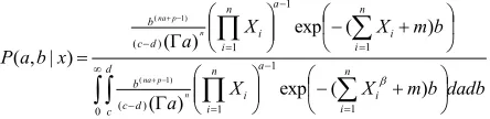
[image:3.612.132.472.497.556.2] [image:3.612.144.467.587.723.2]An another model which has monotone hazard rate is gamma whose probability density function given as
( , | )=
; > 0, , > 0 ……. (11)where a is shape parameter and b is scale parameter. It may also be noted here that for different choice of a, the hazard rate is either increasing or decreasing. When a < 1 the hazard rate is decreasing and a >1 hazard rate is increasing and it reduces to exponential distribution when a=1. The mean waiting time to first birth is
a
/b
. Thus, this model is another competitive model for model A and Model B.The likelihood function for the samples
x
1,
x
2,
x
nis( , | ) =
( )
∗∑ (∏ ) ….. ……..(12)
We follow the same argument as discussed for prior selection in model B and proposed the joint prior for parameter a and b as
p d c mb b m b a g p p ) ( exp , 1; c, d, m, p > 0 ……...(13)
Table 1. DIC for Various Age at Marriage Groups
DIC for Various Age at Marriage Groups
Model 12-15 Years 15-18 Years 18-21 Years 21-24 Years 24 +
years Total age
group
Exponential 8870.2500 17217.7000 8692.0800 2281.1700 780.1960 38018.20
Weibull 8871.7600 17153.5000 8608.7800 2216.4200 753.9790 37891.30
Gamma 8860.7900 17062.9000 8548.7500 2192.7000 753.2990 37770.20
Table 2. Bayes Estimates of the parameters of Gamma distribution
Bayes Estimates of the parameters of Gamma distribution Average Waiting
Time(in- month)
Age at marriage Parameter Posterior
mean
95% H.P.D. Interval
Gamma
12-15 Years a 0.87840 0.81200 0.94840 33.80
b 0.02599 0.02338 0.02869
15-18 Years a 0.72370 0.68570 0.76220 26.87
b 0.02693 0.02496 0.02892
18-21 Years a 0.66170 0.61550 0.70980 20.86
b 0.03172 0.02858 0.03516
21-24 Years a 0.55290 0.48150 0.63070 17.06
b 0.03240 0.02605 0.03924
24 +
years a 0.56590 0.44260 0.70500 17.30
b 0.03271 0.02224 0.04488
Total age group a 0.75880 0.73280 0.78590 26.08
Substituting L
a,b|x
and g
a,b
from (12) and (13) respectively in (10), the joint posterior p
a,b/x
becomes
0 1
1
1 )
(
1 1
1 )
(
) (
exp )
(
) (
exp )
( )
| , (
) 1 (
) 1 (
d
c
n
i i a
n
i i d
c b
n
i i a
n
i i d
c b
dadb b m X X
a
b m X X
a x
b a P
n p na
n p na
(14) It may be noted here that equation (14) cannot be reduced in a
nice closed form. Again to overcome such difficulty we use MCMC method to obtain Bayes estimator of the parameters using Win BUGS software.
Data
To illustrate the proposed procedure, we have taken data from National Family Health Survey-3 held in 2005-06. We all know that onset of menstruation is usually thought to be sign of women’s reproductive maturity. Gondotra and Das (1982) have stated that most of the females in India have their menarche between the ages twelve to fifteen years. Therefore we have considered only those females whose age at marriage was 12 years or more. Another important point to be noted here is that nearly all females who are not using any contraceptive methods and are biologically fits to give birth to their first child conceive much earlier than 7-8 years of their marital duration. Therefore we decided to consider only those females whose marital duration at the survey time was more than nine years. In present study, we are not interested only in average waiting to first conception of the whole data but also interested in effect of age at marriage to the waiting to first conception. Thus the whole data (4461) was divided into five groups according to their age at marriage as 12-15,15-18,18-21,21-24 and 24 + and number of females in these groups are 981, 2006, 1076, 297 and 101.
Model Selection and Estimation of the parameters for considered models
For the estimation of parameters of the considered model, we propose the use of Bayesian method which is based on the posterior distribution. However, for Weibull or Gamma distribution, the posterior distribution of the parameters takes a ratio form that involves integration in the denominator and cannot be reduced in nice closed form when both parameters are unknown. Hence, the Bayes estimators cannot be obtained in closed form. In addition to it the evaluation of the DIC for these models will be tedious. There are several approximation techniques available in literature to solve such types of problem. One of the most widely used methods is Markov Chain Monte Carlo method (MCMC). MCMC is commonly used to evaluate, iteratively, approximate value of some of the complex integrals involving expectation of a function of a random variable. MCMC tool has been incorporated in the Win BUGS (Bayesian inference Using Gibbs Sampling for Windows). One of the important steps in implementation of MCMC via Win BUGS is providing the value of hyper parameters of prior distribution. We first choose the value of hyper parameter such the prior distribution becomes most non informative. Then a large variation of hyper parameters we
which provides the least DIC. After deciding values of the hyper parameter, Bayes estimators for considered models using Win BUGS are obtained and summarized below in the table 2.DIC of the considered model for different age group are also given in Table 1 .
DISCUSSION
From Table 1, we see that for each model the DIC decreases as the age at marriage increases and it is least for the age group 24 years and more. For any given age group, the DIC is least for Gamma model. Between Exponential and Weibull model for early age at marriage group Exponential distribution has slightly smaller DIC as compared to Weibull but the situation is reverse for higher age group. Over all i.e. for the females irrespective of their age at marriage, Gamma distribution has smaller DIC. From Table 2 we see that average waiting timeto first conception (estimated by considering the Gamma model) is highest for the age at marriage group for 12-15 years. As the age at marriage increases, the average waiting time to first conception decreases. This trend continues up to the age group 21-24years. For the age group 24 years and more there is a slight increase in the average waiting time. This trend of variation in the average waiting time to first conception is in conformity with those reported in other studies.
Conclusion
On the basis of DIC criterion, Gamma distribution is found to be the best model among the considered models for the waiting time to first conception. Thus it may be recommended that Gamma distribution can be taken as a suitable model for estimating the average waiting time to first conception than Exponential and Weibull distributions.
REFERENCES
Bhattacharya B.N., Pandey C.M. and Singh K.K. 1986. A model for first birth interval and some social factors”, Mathematical Biosciences, 92:17-28.
Gini, C. 1924. Premieres recherché sur la fecondabilite de la fememe” Proceedings of the International Mathematical Congress, Toromoto, 889-892.
Das Gupta, P. and Hickman, L. 1974. Estimation of the parameters of a type I geometric distribution from truncated observations on conception delays, Mathematical
Biosciences, 22: 75-94.
Henripin, J. La Population, 1954. Canadienne au de but du XVIII e Siecle, Paris, Henry, L. Fondements theoretiques des measures da la fecondite naturelle , Perue de I Instut International de Statistique, 1953, Vol. 21, p. 135-151. Henry, L. 1957. Fecondite et famille models mathematique I,
Population, , Vol. 12, p. 413-444.
Henry, L. 1961 a. Fecondite et famille models mathematique (II) Partic theoretique, Population, Vol.16, p. 27-48. Henry, L. 1961 b. Fecondite et famille models mathematique,
Partic theoretique, Population, , Vol.16, p. 261-282. Ntzoufras, I. 2009. Bayesian Modeling using WinBUGS, A
John Wiley & Sons, INC., Publication
Pathak, K. B. 1999. Stochastic models of family building : An analytical review and prospective issues, Sankhya, Volume 61, Series B, Pt. 2, pp. 237-260
[image:4.612.61.283.94.148.2]Health and Population Perspective and issues, , Vol. 4, p. 171-180.
Pathak, K.B. and Sastri, V.S. 1984. On a method for estimating primary sterilityfrom the data on first conceptive delay.Gujarat Statistical Review, Vol.11, p. 13-20. Potter, R.G. and Parker , M. 1964. Predicting time required to
conceive , Population Studies, , Vol. 18. P. 99.
Sheps, 1964. M.C. On the time required for conception, Population Studies, 1964, Vol. 18, p. 85.
Sheps, M.C. 1965. An analysis of reproductive patterns in an American isolate. Population Studies, 19: pp. 65–80. Singh, S.N. 1961. A hypothetical chance mechanism of
variation in number of births per couple. Unpublished Ph. D. thesis, University of California, Barkeley, USA,. Singh, S.N. 1964. On the time of first birth. Sankhya, Sr.(B),
Vol. 26, p. 95.
Suchindran, C.M. and Lachenbruch, P.A. 1974. Estimates of parameters in a ProbabilityModel for first birth interval, J.
Amer. Statist. Assoc., 69: 507-513.
Vincent, P. 1956. Donnees biometriques sur la conception et la grossesse, Population, Vol. 11, pp.59-85.
Singh P.K., Singh S. K. and Singh U. 2008. Bayes estimator of inverse Gaussian parameters under general entropy loss function using Lindley’s approximation” Communication in Statistics-Simulation and Computation, 37: 1750-1762. Spiegelhalter, D., Best, N., Carlin, B. and van der Linde, A.
2002. Bayesian measures of model Complexity and fit (with discussion), Journal of the Royal Statistical Society B 44: 377-387.