Economics Working Paper Series
2019/013
Investor Sentiment as a Predictor of Market
Returns
Kim Kaivanto and Peng Zhang
The Department of Economics
Lancaster University Management School
Lancaster LA1 4YX
UK
© Authors
All rights reserved. Short sections of text, not to exceed two paragraphs, may be quoted without explicit permission,
provided that full acknowledgement is given.
Investor Sentiment as a Predictor of Market Returns
∗Kim Kaivanto§ and Peng Zhang‡
§Lancaster University, Lancaster LA1 4YX, UK
‡Guizhou Minzu University, Guiyang City, PRC 550025
this version: June 26, 2019
Abstract
Investor sentiment’s effect on asset prices has been studied extensively — to date, without deliv-ering consistent results across samples and datasets. We investigate the asset-pricing impacts of eight widely cited investor-sentiment indicators (one direct, six indirect, one composite), within a unified long-horizon regression framework, predicting real NYSE-index returns over horizon lengths of 1, 3, 12, 24, 36, and 48 months. Results reveal that three of the non-composite indi-cators have consistent predictive power: the Michigan Index of Consumer Sentiment (M ICS), IPO volume (N IP O), and the dividend premium (P DN D). This finding has implications for the widely cited Baker-Wurgler first principal component (SF P C) composite indicator, which extracts information from the full set of six indirect indicators. As the diffusion-index literature shows, this type of wide-net approach is likely to impound idiosyncratic noise into the compos-ite summary indicator, exacerbating forecasting errors. Therefore we create a new ‘targeted’ composite indicator from the first principal component of the three indicators that perform well in long-horizon regressions, i.e. M ICS,N IP O, andP DN D. The resulting targeted composite indicator out-performs SF P C in a market-returns prediction horse race. Whereas SF P C pri-marily predicts Equally Weighted Returns (EW R) rather than Value Weighted Returns (V W R), our new sentiment indicator performs better than SF P C in predicting bothV W R and EW R. This improved performance is due in part to a reduction in overfitting, and in part to incorpo-ration of the direct sentiment indicator M ICS.
Keywords: investor sentiment, market return, predictability, long-horizon regression, bootstrap diffusion index, composite index, overfitting
JEL classification: G12, G17
∗
1
Introduction
Market-return predictability is a well-established area of empirical inquiry. Moreover, it informs cognate questions on the drivers of market risk, the pricing of market risk, and the quantitative modeling of asset prices in general equilibrium. In this paper we undertake a comprehensive investigation of the market-level asset-pricing impacts of eight widely cited investor-sentiment indicators, employing a unified long-horizon-regression framework and an identical sample period for all indicators.
Market-return predictability studies have discovered statistically significant correlations be-tween market returns and various indicators, including short-term interest rates (Fama and Schwert 1977), interest-rate term structure (Keim and Stambaugh 1986, Campbell 1987), past returns (Lo and MacKinlay 1988, Poterba and Summers 1988, Fama and French 1988a, Je-gadeesh 1991), and price-related ratios (Fama and French 1988b, Fama and French 1989, Camp-bell and Shiller 1988, Hodrick 1992).
A further branch of this empirical literature grew from De Long et al.’s (1990) (DSSW) finding that noise traders can prevent well-informed rational traders from arbitraging away dis-parities between market price and fundamental value. DSSW showed that rational arbitrageurs face systematic risk resulting from uncertainty regarding noise traders’ beliefs. By affecting noise traders’ beliefs, investor sentiment can affect asset mispricing marketwide. Accordingly, a substantial post-DSSW literature incorporates proxies for investor sentiment into tests of market-return predictability. These fall in five clusters: survey-based proxy studies (Schmeling 2009 and Lee, Jiang and Indro 2002); tests of the Law of One Price (Baker, Wurgler and Yuan 2011); market-timing studies (Baker and Wurgler 2000); textual analysis of news and social me-dia feeds (Tetlock 2007, Da, Engelberg and Gao 2007, Garcia 2013, and Sun, Najan and Shen 2016); and distillation of common components from multiple indicators (Baker and Wurgler 2006, Baker and Wurgler 2007, Kim Ryu and Seo 2014, Huang et al. 2015, and Han and Li 2017 for international evidence). Empirically, strong positive investor sentiment generally predicts lower returns in the near future, while several studies find that the correlation can turn positive over a longer horizon.
risk factors. For a review, see Baker and Wurgler (2007).
Several indicators share common factor structure, at least in part, despite different ap-proaches to operationalization. Existing empirical studies typically examine the effects of up to three indicators on market returns or portfolio returns, without paying much heed to ensuring comparability with other studies in terms of target return structure, data frequency, sample periods, or model specification.1 Consequently, it is not straightforward to synthesize across studies for drawing general or summative conclusions. Moreover, with a rich list of sentiment indicators successfully predicting cross-sectional returns, it is natural to ask whether such pre-dictability extends to the aggregate market level. When the effect of sentiment is tested, many indicators can be used to explain cross-sectional returns as long as the influence can be rational-ized within a specific sub-market. In contrast, candidates for influential market-level sentiment are more limited. Any candidate indicator must capture latent investor sentiment that (i) affects a significant population of market participants, (ii) becomes reflected in the final price through a clear pricing mechanism, and (iii) has a non-transient effect on aggregate asset prices that is not immediately eliminated by arbitrage.
Consequently, caution must be exercised in choosing sentiment indicators. We undertake a comprehensive investigation of the asset-pricing impacts of seven widely cited non-composite investor-sentiment indicators, employing a unified framework and an identical sample period for all indicators. Results from long-horizon single-factor regressions suggest that three indica-tors (M ICS, N IP O, P DN D) predict market returns well, while the other indicators display little or inconsistent predictive power. This pattern continues to hold even when the economic-fundamentals-reflecting component of the investsentiment indicator is removed through or-thogonalization with respect to a bank of 12 fundamental variables.
Although investor sentiment’s posited effect on asset prices has been studied extensively, the time lag with which investor sentiment is expected to become impounded into asset prices is neither theoretically nor empirically well understood.2 It has also been found that the effects of certain investor-sentiment proxies tend to reverse over longer horizons. Yet literature on the
1
Existing literature on the effect of investor sentiment in market return predictability consists of studies that (i) target various market index returns, including value-weighted and equal-weighted NYSE, S&P500, DJIA, AMEX, NASDAQ, RUSSEL3000, and different combinations of these indices; (ii) analyze samples of frequencies from half-hour to annual data; (iii) focus on a variety of sample lengths between four years and a century; and (iv) adopt multiple models for the estimation. The story on investor sentiment and cross-sectional returns is even more diverse.
time-lag dimension remains limited. We implement long-horizon double-factor regressions to investigate the time dimension of investor-sentiment’s effect on market returns. For each of the horizons T ∈ {1,3,12,24,36,48} we estimate a specification that controls for average returns realized up to time T −1, thereby revealing whether the sentiment indicator retains predictive power on month-T returns that is independent of its effect on returns in the T −1 preceding months. The three indicators that show strong predictive power in single-factor regressions (M ICS,N IP O,P DN D) all demonstrate consistent, long-lasting predictive power in double-factor regressions. But we observe little evidence of eventual reversal, unlike some previous studies. This is our second contribution.
Lastly, the results of the predictive-power tests may be refined further within the ‘diffusion index’ framework. The common tendencies in a large collection of time series may be summarized by a limited number of ‘diffusion indices’, which may be constructed using a variety of different techniques, including e.g. principal component analysis, dynamic factor analysis, partial least squares, and least-angle regression. Diffusion indices may be used to improve the performance of forecasting models, or to mitigate overidentification problems. In the area of investor sentiment, Baker and Wurgler’s (2006, 2007) widely cited approach constructs a diffusion index from the first principal component (SFPC) of all six indirect investor-sentiment indicators. However, as Bai and Ng (2008) argue, indiscriminate inclusion of predictors in the diffusion index may introduce too much idiosyncratic noise, thereby leading to potential overfitting and exacerbating forecasting errors.3 We follow Bai and Ng (2008) in selecting a subset of targeted predictors, using significant predictive power as a marker for inclusion in the subset, from which we construct a new diffusion index (T3-SF P C) that is the first principal component of this subset. In a market-returns prediction horse race, our new index consistently beats the SF P C index of Baker and Wurgler (2006, 2007). This improved control of overfitting is our third contribution. The sequel is structured as follows: Section 2 introduces the data. Methodology is summa-rized in Section 3. Sections 4 and 5 report results from single-factor and double-factor regressions over multiple horizons, respectively. We extract new ‘targeted’ diffusion indices in Section 6 and test their predictive power against the benchmarks of Baker and Wurgler (2006, 2007). Section 7 concludes.
2
Data
We use real NYSE index returns to represent the market return. Both equal-weighted and value-weighted monthly NYSE index returns are obtained from the Center for Research in Security Prices (CRSP), which are then adjusted with the Consumer Price Index (CPI) into real returns.4 For investor-sentiment indicators, our choice is mainly constrained by data availability. Most of the indicators are only available over relatively limited time intervals and in frequencies that are not uniformly comparable. Striking a balance between the number of indicators and achievable sample size, we elect to focus on eight monthly indicators from January 1978 through to December 2007. These indicators are introduced in the following subsections, including direct, indirect and composite sentiment measures.
2.1 Direct sentiment measures
The most straightforward, direct indicators of sentiment are provided by survey data. Shiller (1999) suggests that the Yale School of Management Stock Market Confidence Indices can reflect the attitudes of institutional investors. Qiu and Welch (2006) show that data from the UBS/Gallup surveys can explain returns, particularly small-stock returns and returns of stocks held disproportionately by retail investors. Similar findings have also been obtained by Lemmon and Portniaguina (2006) with data from both the Index of Consumer Confidence and the University of Michigan Consumer Confidence Index. Brown and Cliff (2005) find significant long-horizon explanatory power in the Investors Intelligence survey.
Since survey-data availability is the main constraint on sample size, we give data availability the highest priority when choosing among different surveys. As a result, we use the Index of Consumer Sentiment from the University of Michigan Consumer Confidence Index. Although the survey was not originally designed to reflect investor sentiment in asset markets — but rather, to gauge general consumer confidence — it serves the sample-size-maximization objective in that it has been compiled consistently, without interruption, for longer than any other comparable survey. At an annual frequency the survey is available as far back as 1952, while at a monthly frequency the survey is available from January 1978 onward.
The Michigan Index of Consumer Sentiment (M ICS) indicator is calculated as a linear 4
transformation of the percentages of positive and negative responses on five telephone-survey questions. The five questions cover (i) change in perceived household financial situation over the last year, (ii) expected year-ahead change in household financial situation, (iii) expected year-ahead national financial business conditions, (iv) expected national business conditions (continuous good times vs. periods of widespread unemployment or depression) over the coming 5 years, and (v) current purchasing conditions for major household durable items.
2.2 Indirect sentiment measures
We also adopt the following six indirect indicators from Jeffrey Wurgler’s online data library, including closed-end-fund discount (CEF D), NYSE turnover (T U RN), IPO volume (N IP O), IPO first day return (RIP O), net equity issuance fraction in total issuance (N EIF), and divi-dend premium (P DN D). The indicators are constructed as follows.
Closed-end fund discount: Zweig (1973) uses the discount to verify that prices are likely to deviate from fundamental values when ‘noise’ is present. DeLong et al. (1990) attribute the discount to the fact that closed-end funds are mainly held by individual investors and that the noise brought by these investors will lead to an extra risk premium. Lee et al. (1991), Neal and Wheatley (1998) and Swaminathan (1996) find evidence that the discount is a measure of investor sentiment and can help explain market returns. The closed-end-fund discount (CEF D) indicator is calculated as the average percentage difference between the market-based Net Asset Value of the shares held by the closed-end funds and the prices at which closed-end funds’ shares change hands.
Market liquidity: Empirical studies have long found coexistence of higher liquidity and lower future returns5. Baker and Stein (2004) argue that liquidity provides an indicator of the presence or absence of irrational investors who face short-sale constraints and are active only in optimism. Scheinkman and Xiong’s work (2003) also points out the link between sentiment and market liquidity. NYSE turnover (T U RN) is obtained as the natural logarithm of the ratio of reported share volume over average number of shares listed on NYSE.
cause high post-IPO returns. IPO volume (N IP O) records the number of IPOs in the month. IPO first-day return (RIP O) records the average first-day percentage return of all IPOs in the month.
New equity issuance: Given that IPOs are just one indicator of equity financing, a more general indicator of investor sentiment (in stock markets) can be gauged by the fraction of equity issuance to total asset issuance. Baker and Wurgler (2000) find a negative relationship between equity issuance and stock market returns, and attribute this relationship to issuers shifting between equity and debt to minimize the cost of financing. New-equity-issuance fraction (N EIF) is the proportion of new equity issued out of total issuance of equity and debt.
Dividend premium: Baker and Wurgler (2004a,b) argue that since dividend-paying equities have characteristics like coupon bonds, they represent ‘safety’ compared to dividend-nonpaying equities. As a result Baker and Wurgler (2006, 2007) argue that when investors perceive high risk level and look for safety, investor demand for dividends will drive prices of the dividend-paying and dividend-non-dividend-paying stocks apart. The dividend premium (P DN D) is calculated as the log difference of the value-weighted average market-to-book ratios of dividend payers and dividend non-payers.
2.3 Composite sentiment measure
The principal component sentiment index (SF P C), which is based on the first principal com-ponents of the six standardized6 indirect indicators, as calculated in Baker and Wurgler (2007). Note that SF P C may be understood as a ‘diffusion index’: i.e. a linear summary of the common tendencies in a large collection of time series. In many-predictor forecasting problems the diffusion-index method is widely accepted for its ability to reduce dimensionality, overcome overfitting, and improve forecasting accuracy (see e.g. Stock and Watson 2002, Boivin and Ng 2006, and Ludvigson and Ng 2007, among others).7
2.4 Orthogonalized sentiment indicators
Raw sentiment indicators may contain not only information reflecting investor sentiment but also macroeconomic fundamentals (Baker and Wurgler 2006, 2007, Brown and Cliff 2005, and Neal and Wheatley 1998). In order to exclude the component reflecting fundamentals, indicators
6
Here standardization means subtracting the mean and then dividing by the standard deviation.
are standardized and then orthogonalized with respect to fundamental variables prior to being used in further analysis. We employ two sets of fundamental variables. The first set follows Baker and Wurgler’s (2006, 2007) consumption-based asset-pricing approach in incorporating: growth in industrial production; real growth in durable, non-durable, services and total con-sumption; growth rates in employment, CPI; and an NBER recession dummy variable. The second set follows Brown and Cliff’s (2005) and Neal and Wheatly’s (1998) conditional asset pricing approach in incorporating: 1-month real US Treasury bill return; the difference between 3-month and 1-month real US treasury bill returns; the difference between 10-year and 3-month real US treasury bill returns; and the default spread between yields on Moody’s Baa- and Aaa-rated corporate bonds. Data series for the first set have been obtained from Jeffrey Wurgler’s online data library, whilst data series for the second set have been obtained from the US Federal Reserve. F tests show that the two sets of variables are jointly significant in explaining all sentiment indicators. Criteria including AIC and BIC suggest retaining both sets.
We use two parallel approaches for generating orthogonalized sentiment indicators. In the first approach all twelve fundamental variables are retained and therefore each orthogonalized sentiment indicator excludes the same fundamental information. In the second approach each sentiment indicator is orthogonalized with respect to only those fundamental variables that are statistically significant explanators of the indicator in question. Both approaches lead to qualitatively identical results in further analysis.
2.5 Sample characteristics
Table 1 summarizes the sample characteristics of the seven non-composite sentiment indicators (one direct and six indirect). All sentiment indicators exceptM ICS have positive excess kurto-sis values. The skewness values of all sentiment indicators exceptM ICS andCEF D show that investor sentiment is right skewed,8 suggesting fat tails for bullish investor sentiment.9 Intu-itively, since previous studies find a negative correlation between investor sentiment and market returns,right-skewed investor sentiment is consistent with thenegative skewness in asset returns
(e.g. Cont 2001, Jackwerth and Rubinstein 1996). Indeed a new literature specifically tests the 8
CEF D and P DN D are supposedly negatively correlated to investor sentiment whilst all other variables are positively correlated to sentiment. If the correlations were perfect, the skewness for distribution of investor sentiment would be opposite to those ofCEF DandP DN Dand be the same as those of other indicators.
relationships between investor sentiment and return skewness. For instance, Han (2008) shows that the level of investor sentiment affects the skewness of S&P 500 return and the slope of index option volatility smile.
[image:10.595.146.453.333.458.2]Table 2 summarizes the sample characteristics of the orthogonalized sentiment indicators. Again, kurtosis values are inflated. Because the orthogonalized indicators come from the residu-als of orthogonalization, the means are all extremely close to 0. Compared to Table 1, the signs on skewness and excess kurtosis statistics remain unchanged after orthogonalisation for every sentiment indicator exceptCEF D. However the values of the third and fourth central moments are often different from those in Table 1, showing that the distributional features of sentiment indicators are only partly preserved after excluding the impact of macroeconomic fundamentals.
Table 1: Summary statistics of original indicators
Mean Median S.D. Skewness Kurtosis
M ICS 88.0033 90.9000 12.0700 -0.5570 -0.1308
CEF D 8.6801 8.4950 5.6863 0.7743 0.4117
T U RN 0.6816 0.5970 0.3518 1.8182 4.5544
N IP O 32.1667 26.0000 24.5374 0.9375 0.4307
RIP O 19.2269 14.1000 19.8890 2.4491 6.9768
N EIF 0.1609 0.1379 0.1097 1.4860 2.1447
P DN D -13.3101 -12.8300 10.2970 -0.9999 3.5731
[image:10.595.147.451.547.673.2]This table shows summary statistics for the data of original sentiment indicators used in the analysis. The full monthly sample contains 360 observations from Januaray 1978 through December 2007.
Table 2: Summary statistics of orthogonalized indicators
Mean Median S.D. Skewness Kurtosis
M ICS⊥ 0.0000 0.0119 0.5092 -0.1215 -0.0780
CEF D⊥ 0.0000 0.0810 0.5830 -0.5657 -0.1578
T U RN⊥ 0.0000 -0.0326 0.4194 1.1033 5.4288
N IP O⊥ 0.0000 -0.1316 0.7371 1.1396 1.8480
RIP O⊥ 0.0000 -0.0765 0.8699 1.3997 3.5062
N EIF⊥ 0.0000 -0.0634 0.5779 0.6605 1.8671
P DN D⊥ 0.0000 0.0215 0.6966 -1.0584 3.4518
This table shows summary statistics for the data of sentiment indicators orthogonalized with twelve fundamental variables. The full monthly sample contains 360 observations from Januaray 1978 through December 2007.
original indicators; Panel B contains orthogonalized indicators. As discussed above, the signs on skewness and kurtosis remain unchanged after orthogonalisation in all cases exceptCEF D. However the distinctions between Panels A and B suggest that excluding the influence of fun-damental variables clearly changes the distributions of sentiment indicators.
Tables 3 and 4 show the correlation structure between sentiment indicators. As found in the literature (e.g. Brown and Cliff 2004 and Baker and Wurgler 2006), correlations between different indicators are usually small in magnitude. The pairwise correlations are all below 0.5. This is consistent with the notion that indicators are noisy proxies for investor sentiment and reflect investor sentiment in partial and disparate ways. As discussed by Baker and Wurgler (2006), each indicator contains not only a ‘sentiment component’ but also‘idiosyncratic, non-sentiment-related components’ (Baker and Wurgler 2006, p.1656). For instance, the survey indicator (M ICS) reflects consumer confidence in general, and thus contains information on e.g. employment conditions, which may be correlated with the broader economy in addition to the stock market. Indirect sentiment indicators reflect different mechanisms, including market-timing behaviour, liquidity-provision activity, safety seeking, and the noise-trader risk premium. Thus each indicator contains idiosyncratic noise components which are not directly related to investor sentiment and hence lead to small pairwise correlations. This has an important implication for our empirical tests: we expect to find nonuniform results across indicators due to different, possibly stochastic levels of noise across indicators.
[image:11.595.76.531.553.687.2]Similar results are obtained with original indicators and orthogonalized indicators, suggesting a robust correlation structure that is not merely a reflection of common fundamentals.
Table 3: Correlation of original indicators
M ICS
CEF D
T U RN
N IP O
RIP O
N EIF
P DN D
M ICS
1
CEF D
-0.3376
1
T U RN
0.2923
-0.3472
1
N IP O
0.2941
-0.2044
-0.1656
1
RIP O
0.1224
0.2978
-0.0365
-0.0024
1
N EIF
-0.3530
0.3282
-0.4663
0.3353
0.1728
1
P DN D
-0.1410
-0.1385
-0.0094
-0.3765
-0.4560
-0.4326
1
(a) Panel A: Histograms of original sentiment indicators
[image:12.595.116.481.78.387.2](b) Panel B: Histograms of orthogonalized sentiment indicators
Table 4: Correlation of orthogonalized indicators
M ICS⊥ CEF D⊥ T U RN⊥ N IP O⊥ RIP O⊥ N EIF⊥ P DN D⊥
M ICS⊥ 1
CEF D⊥ -0.2642 1
T U RN⊥ 0.2529 -0.0530 1
N IP O⊥ 0.1969 0.0224 0.2269 1
RIP O⊥ -0.0023 0.1230 0.0518 0.0713 1
N EIF⊥ -0.0957 0.2302 0.0152 0.3603 0.1816 1
P DN D⊥ -0.1058 -0.1438 -0.0990 -0.3571 -0.4507 -0.3569 1
This table shows the correlation coefficients of orthogonalized indicators.
3
Methodology
3.1 Model specification
Although investor sentiment’s effect on asset prices has been studied extensively, giving rise to a rich empirical literature, theoretical models nevertheless offer no guidance as to the length of the time horizon over which sentiment becomes impounded into asset prices. Evidence has been found in both short-horizon and long-horizon analysis. We first follow practice in the market-return predictability literature and conduct our analysis over multiple horizons. Existing studies of market-return predictability mainly employ three long-horizon model specifications:
(i) Campbell and Shiller (1988) adopt a VAR model as follows
zt=Azt−1+υt
where zt is a matrix consisting of return and dividend-price ratio. Long-horizon analysis is implicit in the model.
(ii) Fama and French (1988a, 1988b) use single-factor regression to explain future multiple-period returns with past return or current dividend-price ratio, as in
r(t, t+T) =α(T) +β(T)Y(t) +ε(t+T)
where r(t, t+T) is future return (with T set to various horizon lengths), Y(t) represents past return or the dividend-price ratio, and ε(t+T) is the error term.
returns with the sum of lagged returns as a single regressor, as in
Rt=ak+bk K
X
i=1
Rt−i+uK,t
where Rt is the next-period return, K
P
i=1
Rt−i is the sum of lagged returns, and uK,t is the error term.
Further discussion of the similarities across models and the advantages of each specification can be found in Hodrick (1992) and Campbell (2001).
In this paper we first follow the Fama and French (1988b) model by estimating single-factor regressions over multiple horizons. We examine the null hypothesis that investor-sentiment indicators have no predictive power for market returns. We follow Fama and French (1988b, 1989) in setting the horizon lengths to 1, 3, 12, 24, 36, and 48 months. In Section 4, we run the single-factor regressions by regressing futurek-month average returns on a constant and an indicator of investor sentiment.
1 k
k
X
i=1
rt+i=c(k)+β(k)St+(tk) (1)
where:
(i)rcan refer to equal-weighted return (EWR) or value-weighted return (V WR) of the NYSE index;
(ii) S represents one of the sentiment indicators and can refer to M ICS,CEF D, T U RN, N IP O,RIP O,N EIF, orP DN D;
(iii) krepresents the horizon length and can take the values 1, 3, 12. 24, 36, or 48.
(iv) the coefficient β(k) represents how sensitive the future return is to investor sentiment, given the horizon length k. If β(k) is statistically significant then evidence of predictive power in the investor-sentiment indicator is present.
time-decaying component in the price process or aggregation biases.
1 k
k
X
i=1
rt+i =c(k)+α(k) 1 k
k
X
i=1 rt−1+i
!
+β(k)St+(tk) (2)
The introduction of first-order lagged (future) returns means that estimating equation 2 for different horizons k ∈ {1,3,12,24,36,48} allows the analysis to search for the time period over which investor sentiment becomes impounded into market returns. For example, when k is set to 3, the coefficient β(k) will capture the effect of St on 13
3
P
i=1
rt+i that is not already
incorporated into 13 3
P
i=1
rt−1+i, i.e. rt, rt+1, and rt+2. [KK: I think the original notation’s
subscript was incorrect (I have commented it out above). Please verify that my
change here is correct. PZ: I was trying to point out the new component in 13
3
P
i=1 rt+i
compared to 13
3
P
i=1
rt−1+i.] If β(k) is statistically significant, then it can be claimed that the St retains predictive power on 3-month-ahead returns independently of any effect via current-period, 1-month-ahead, and 2-months-ahead returns. By assembling estimation results for mul-tiple horizon lengths, we map the predictive power of different sentiment indicators along the time line.
The horizon lengths we use here contain both monthly and long-horizon frequencies. As is well known in the literature on long-horizon regression, the overlapping dependent variables will introduce strong autocorrelation within the residuals and therefore lead to biased and in most cases inconsistent estimates for least square coefficients (see e.g. Valkanov 2003). Furthermore, the distributions of the estimated coefficients are often not normal, together with the calculated standard errors being incorrect. As a result standard hypothesis tests do not provide reliable results. We use bootstrap methods to correct for the bias, as detailed in the online appendix.
4
Single-factor regressions
Tables 5 and 6 present the sentiment-indicator coefficients from regression Equation 1. Table 5 is based on original investor-sentiment indicators, whereas Table 6 is based on orthogonalized sentiment indicators. In both tables coefficient estimates βd(k) are reported, with the adjusted
p-values from bootstrap distributions in parentheses. Eachp-value below 5% is denoted by an asterix (*).
the horizon length increases. Consequently, little may be gained by dwelling on long-horizon regression R2 values. Due to this fact, we follow Fama and French’s (1988a) practice of report-ing only coefficient estimates and significance levels, omittreport-ing R2 values from Tables 5 and 6. Instead, we discuss the R2 at 1-month horizon briefly.
In line with the evidence from single-factor models of return predictability (e.g. Fama and French 1988b), the magnitudes ofR2 at 1-month horizon are very small. R2 values remain below 5% for all seven indicators, and this is true both before and after orthogonalization. We leave R2 values’ market-efficiency implications to readers.10
4.1 Signs
Although theory (e.g. Shiller et al. 1984, Summers 1986, and Scheinkman and Xiong 2003) places no restrictions on the horizon over which investor sentiment may affect asset prices, it is understood that when investor sentiment is high, current asset prices will be driven up and therefore reduce expected future returns. When investor sentiment is low the opposite is generally true. An empirical question therefore is: How long does it take for the market to demonstrate such a negative correlation between investor sentiment and future returns? The long-horizon structure in our model provides an opportunity to answer this question.
Theory predicts positiveβd(k)for all indicators that reflect sentiment negatively (CEF Dand
P DN D), and negative βd(k) for all indicators that reflect sentiment positively (M ICS,T U RN,
N IP O,RIP O andN EIF). In the rest of this section we discuss whether the signs of βd(k)stay
as expected over various horizons.
Most coefficient estimates’ signs are consistent with those predicted by and as found in the existing literature (74 out of 84 coefficients across Tables 5 and 6).
All but one of the coefficients with the unexpected sign are statistically insignificant. There is weak evidence of a long-term reversal pattern for predicting V WR with N IP O and N EIF, although few of these negative coefficients are statistically significant.
Perhaps the most interesting finding regarding the signs of coefficients comes from RIP O. The correlation often stays positive for short horizons (1 month and 3 months) — contrary to theoretical predictions. The correlation turns negative for longer horizons. While behavioral asset pricing theories and anecdotal evidence generally agree that firms and investment banks
10
T able 5: Co efficien ts of original sen timen t indicators and p -v alues This table records the estimated co efficien t and p -v alues in the regress ion equation 1 k k
P i=1
rt+
T able 6: Co efficien ts of orthogonalized se n timen t indicators and p -v alues This table records the estimated co efficien t and p -v alues in the regress ion equation 1 k k
P i=1
rt+
are ‘timing’ the market by launching IPOs when investor sentiment is high, therefore entailing that high RIP O will be followed by low future returns, our empirical findings suggest that the prediction is true only for longer horizons. In other words, in the short term there must exist more complicated dynamics between RIP O and investor sentiment or other sentiment indicators. First, RIP O is also part of market return and may be driven up by low sentiment in previous periods. Second, it is widely agreed that IPO pricing is extremely difficult and that even seasoned professionals — including IPO-underwriting investment banks — can make pricing mistakes, and that underwriter’s pricing decision is conditioned by an asymmetric loss function. Therefore high RIP O may simply be a consequence of IPO undervaluation instead of resulting from high demand for IPO equities driven by high investor sentiment. Last but not least, it is possible that RIP O affects returns with a lag. As there is a long lead time for preparing an IPO, highRIP Owill make initial public offerings attractive but can only lead to a wave of new IPOs with several months’ delay. In this way IPO volume (N IP O) will lagRIP O. If N IP O constitutes a good proxy of investor sentiment, then RIP O will also affect future returns, but only in a lagged way. These relationships are borne out in the next subsection.
4.2 Significance
First, the seven indicators show different levels of predictive power. The average numbers of significant coefficients across Tables 5 and 6 are 8.5 for M ICS, 1 forCEF D, 4.5 forT U RN, 7 forN IP O, 2.5 for RIP O, 4 forN EIF, and 7.5 for P DN D.
As the only direct sentiment indicator, survey data (M ICS) shows strong predictive power across the full range of horizons. This finding is particularly noteworthy given that M ICS achieves such predictive performance despite being designed to capture general consumer senti-ment rather than any factors specific to stock-market returns. Since comparatively few studies have focused on predicting market returns with survey data, our results validate survey-based sentiment indicators for use in future studies. It is entirely possible that surveys focusing specif-ically on investor sentiment can further improve predictive performance.
Number of IPOs (N IP O) and dividend premium (P DN D) also show strong predictive power. N IP O significantly predicts EWR across horizons, whist it also offers some weak evi-dence ofV WR predictivity. P DN D performs well over horizons from 3 months up to 3 years.
Net equity issuance (N EIF) fails to predict market returns in its original form, but its performance improves after orthogonalization.
The closed-end fund discount (CEF D) shows little predictive power, suggesting that its performance in cross-sectional studies (Zweig 1973, DeLong et al. 1990) does not generalize to aggregate market returns.
Compared to M ICS, N IP O and P DN D, the predictive performance of T U RN, N EIF and RIP O appears distinctly less systematic and more variable. We argue that the liquidity-based T U RN may reflect heterogeneity in investor beliefs, which does not necessarily lead to bullish or bearish investor sentiment at the aggregate-market level since bullish belief and bearish belief may well cancel out. N EIF may capture firm-level decisions — the choice between debt financing and equity financing is influenced not only by investor sentiment, but notably by tax policy (e.g. tax-deductible interest cost) and capital structure (e.g. debt ceiling). Moreover N EIF may reflect investor sentiment only to the extent that the equity market is more sensitive to sentiment than the bond market. As discussed in last subsection, the dynamics betweenRIP O and market returns may go beyond a simple form of return predictability, involving complex leading-following order, IPO pricing-error, and lagged influence.
Second, several indicators predict EWR better than V WR. N IP O consistently predicts EWRover all horizons, but forV WRits predictive power is very limited. M ICSperforms better in explaining future EWR thanV WR, particularly after orthogonalization. Previous emipirical studies show that new stocks and small stocks are generally more affected by investor sentiment. Theoretical work argues that these stocks are harder to value and more difficult to arbitrage and hence are more likely to be subject to mispricing.11 Empirical work on this question has successfully made use of a variety of sentiment indicators.12 As new stocks and small stocks have lower capitalization levels, they contribute more to equal-weighted index returns than to value-weighted index returns. Therefore compared to V WR, EWR is better suited to capturing the effect of investor sentiment on new and small stocks. Overall our results support the conjecture that small stocks are more prone to being affected by sentiment than large stocks.
Third, considerable predictive power is found in P DN D, primarily at horizons of 1 year or longer. RIP O becomes significant in explaining V WR for horizons over 2 years. Market turnover (T U RN) predicts returns at horizons in excess of 1 year. We interpret these findings
11
A good review on this literature can be found in Baker and Wurgler (2007).
as evidence that these indicators predict market returns with a lag.13 When investors seek to switch to dividend-paying firms they are not only searching for ‘safety’ in the immediate future but also ‘safety’ in the more distant future. Therefore P DN D reflects investor attitude toward the more distant future, and consequently the dividend premium affects future returns with a lag. With regard to RIP O, several studies point out that it leads IPO volume (N IP O). As N IP O predicts future returns, it is natural for RIP O to predict returns with a lag.
4.3 Robustness
Above we showed that these empirical results are robust to two independent implementations of orthogonalization (with all 12 macroeconomic variables and with the significant subset of the 12 variables for each indicator). In this section we report additional robustness checks, which confirm that our findings are not an artifact of any particular choice made in implementing the bootstrap. We explore the robustness of the results appearing in Tables 5 and 6 using three different approaches: (i) by varying the bootstrap’s moving block length, (ii) by employing a paired moving block re-sampling technique inspired by Freedman (1981, 1984), and (iii) by combining (i) and (ii). We first introduce each approach and then briefly discuss the associated results, especially how they compare with those appearing in Tables 5 and 6.
First, given the moving-average structure of overlapping returns, it is arguably more appro-priate to choose the block lengths according to the horizon lengths. For instance, at 3-months horizon length the return in Equation 1 or 2 becomes 13
3
P
i=1
rt+i and therefore is expected to have the characteristics of a M A(2) process. As a result it is likely that the residuals also follow the M A(2) process. In this case choosing a block length of 3 in the moving block bootstrap will better capture the structure of the original data. By setting the block length equal to the horizon length (1, 3, 12, 24, 36, and 48 months respectively) we obtain the first set of robustness-test results.
Second, since model misspecification in the single-factor regression (Equation 1) is almost certainly present, the influence of any omitted predictor will likely be captured in the residuals. Unless all the possibly omitted predictors are independent of the sentiment indicator, there will be dependence between the regressor and the residuals. As discussed by Freedman (1981, 1984), in such cases it is important to calibrate such dependence within the data generating process
13
(DGP) of any bootstrap implementation in order to achieve satisfactory asymptotic results. In fact, Freedman (1984) proves that assuming a joint distribution between the regressors and residuals and bootstrapping them in pairs is at least as sound as the conventional asymptotic methods.
This article is by no means the first study to pair regressors and residuals in the bootstrap or to resample the pair from blocks. Li and Maddala (1997) implicitly follow this approach and combine it with a parametric DGP for the regressors. MacKinnon (2006) suggests the use of a similar approach for all multivariate models. Our second robustness check is constructed by pairing regressor and residuals in the moving-block resampling.
In the third approach, we make both changes mentioned above to the bootstrap DGP. Since robustness tests only manipulate the bootstrapping process, coefficient estimates from Equation 1 remain unchanged and the level of robustness is reflected solely in variations of bootstrapped standard deviations and the resulting p-values. In what follows we briefly discuss the headlines of the robustness evidence to show that the originally observed patterns persist across all three robustness-check variations.
Compared with the results reported in Table 5, the robustness-check variations have at most a marginal impact upon the number of significant coefficients. For M ICS there is a slight decrease from 10 to 9, 10 and 10. For CEF D the change is ambiguous, from 1 to 0, 2 and 3. For T U RN the number changes from 6 to 6, 5 and 5. For N IP O the number stays at 6. For RIP O there is an increase from 3 to 3, 5 and 4. For N EIF the change is ambiguous, from 1 to 0, 2 and 2. ForP DN D there is a marginal decrease from 8 to 7, 8 and 8.
A similar pattern emerges from the robustness checks applied to orthogonalized data in Table 6. For M ICS⊥ there is a slight decrease from 7 to 6, 7 and 8. For CEF D⊥ there is a slight decrease from 1 to 0, 1 and 1. For T U RN⊥ from 3 to 3, 4 and 4. For N IP O⊥ the number increases from 8 to 8, 9 and 9. ForRIP O⊥there is a change from 2 to 3, 1 and 1. For N EIF⊥ the number changes from 8 to 6, 8 and 8. For P DN D⊥ there is a marginal decrease from 7 to 7, 6 and 7.
P DN D,T U RN and RIP O remains in the robustness-check variations.
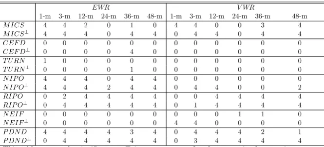
[image:23.595.129.466.434.592.2]Table 7 reports a further robustness summary measure: the count, across the four bootstrap implementations, of the number of times the coefficient is significant in a regression of market returns on sentiment. This count is reported for each indicator, in both original and orthog-onalized forms, for horizon lengths of 1, 3, 12, 24, 36, and 48 months, separately for equally-weighted returns (EWR) and value-weighted returns (V WR). Perfectly consistent (perfectly robust) results generate counts of 4 (all significant) or 0 (all non-significant). Least-consistent (least-robust) results generate a count of 2. The significant-coefficient counts reported in Table 7 show that in most cases the four bootstrap implementations lead to the same conclusion: ‘4’ or ‘0’ appears in 143 out of 168 (85.1%) indicator-horizon-return-type combinations. Meanwhile the value ‘2’ appears in only 11 out of 168 (6.5%) combinations. At the level of individual indicators, N IP O/N IP O⊥ displays the most consistency, then P DN D/P DN D⊥, after which M ICS/M ICS⊥ and RIP O/RIP O⊥ fall in third place. But even this third-place category musters perfect consistency for 87.5% of the models. We infer that the globally best-performing indicators — M ICS,N IP O, and P DN D — achieve robust predictive success.
Table 7: Number of significant coefficients across four bootstrap implementations (single-factor regression)
EWR V WR
1-m 3-m 12-m 24-m 36-m 48-m 1-m 3-m 12-m 24-m 36-m 48-m
M ICS 4 4 4 4 4 4 0 4 0 0 3 4
M ICS⊥ 4 4 4 4 4 4 0 1 0 0 0 3 CEF D 0 0 0 1 2 3 0 0 0 0 0 0
CEF D⊥ 0 0 0 0 0 0 0 0 0 0 0 3 T U RN 2 1 0 2 2 0 0 1 2 4 4 4
T U RN⊥ 0 0 0 4 4 4 0 0 0 0 0 2
N IP O 4 4 4 4 4 4 0 0 0 0 0 0
N IP O⊥ 4 4 4 4 4 4 0 4 4 3 0 0
RIP O 0 0 0 0 0 0 0 0 2 4 4 4
RIP O⊥ 0 0 0 1 0 0 0 0 0 4 2 0
N EIF 0 0 0 0 0 0 0 0 0 0 2 3
N EIF⊥ 0 0 4 2 3 0 4 4 4 4 4 1 P DN D 0 4 4 4 4 3 0 0 4 4 4 0
P DN D⊥ 0 0 4 4 4 0 0 2 4 4 4 0
This table reports the significant-coefficient count across four bootstrap implementations of regressing EWR and VWR, respectively, on each sentiment indicator in turn, at horizon lenghts of 1, 3, 12, 24, 36, and 48 months. For each indicator-return-horizon combination the four bootstrap implementations are: one primary and three robustness-check variants. Perfect robustness is indicated by a significant-coefficient count of either 4 or 0. A count of 2 indicates the least-robust case. Results are reported for both original and orthogonalized variants of each indicator.
5
Impounding horizon: double-factor regressions
indicators, whereas Table 9 is based on orthogonalized sentiment indicators. Both tables report
d
β(k)-coefficient estimates, with bootstrapped p-values in parentheses. Each < 5% p-value is marked with an asterix (*).
We interpret results in Tables 8 and 9 through (i) contrasting the results with those obtained in Section 4 (single-factor regression), and (ii) pointing out that by controlling for average returns realized up to time T-1 (T representing horizon length), the specification of double-factor regression reveals whether the sentiment indicator retains predictive power on month-T returns that is independent of its effect on returns in all the T-1 proceding months. The latter approach offers additional and explicit searches for (a) the time lag with which investor sentiment is expected to become impounded into market prices and (b) the duration of investor sentiment’s influence on market prices before such influence gradually decays to zero.
For reasons discussed in Section 4, we follow Fama and French’s (1988a) practice of reporting only coefficient estimates and significance levels, omitting R2 values from Tables 8 and 9. Due to the additional predictor, the R2 at 1-month horizon is generally higher than that in Section 4. However the typical values ofR2 still fall below 10%.
5.1 Signs
The coefficient signs reported in Tables 8 and 9 generally support the hypothesis that investor sentiment is negatively correlated with future returns (70 out of 84 coefficients in Table 8 and 67 out of 84 in Table 9). However slightly greater inconsistency is present, compared to single-factor regression results. The inconsistency is particularly prominent in CEF D and N EIF.
All but one of the coefficients with the unexpected sign are statistically insignificant. There exists weak evidence of a long-term reversal pattern from CEF D and N EIF, although few reverse-signed coefficients are statistically significant.
The direct indicatorM ICS has negative coefficients in all 24 regressions across Tables 8 and 9.
The six indirect indicators also have expected signs in most cases. The fraction of expected signs is 58/72 (81%) in Table 8, and 55/72 (76%) in Table 9. Compared to the fractions from single-factor regressions, the decreases mainly come from two indicators: CEF D and N EIF. The former has only 5 (Table 8) and 3 (Table 9) coefficients with the expected positive signs, while the latter has only 6 (Table 8) and 8 (Table 9).
T able 8: Co efficien ts of original sen timen t indicators and p -v alues This table records the estimated co efficien t and p -v alues in the regress ion equation 1 k k
P i=1
rt+
i = c ( k )+ α ( k )( 1 k k
P i=1
rt−
T able 9: Co efficien ts of orthogonalized se n timen t indicators and p -v alues This table records the estimated co efficien t and p -v alues in the regress ion equation 1 k k
P i=1
rt+
i = c ( k )+ α ( k )( 1 k k
P i=1
rt−
4) persist at 1-month horizon in Table 9.
5.2 Significance
As in the single-factor regressions, there are marked differences between indicators. The average number of significant coefficients across Tables 8 and 9 is 8 for M ICS, 0.5 for CEF D, 0 for T U RN, 6 forN IP O, 9 forRIP O, 1 forN EIF, and 9.5 forP DN D. These results clearly show that the indicators are far from equally informative over longer horizons.
The indicators that perform well in single-factor regressions —M ICS,N IP Oand P DN D — retain strong predictive performance over and above market return’s self-explanatory power. The performance of RIP O is better in Tables 8 and 9 than in Tables 5 and 6. As in single-factor regressions, CEF D fails to predict future returns. Relative to single-factor regressions, the predictive power of T U RN and N EIF fades once the autocorrelation in market return is taken into account.
EWR is still marginally better explained by sentiment indicators than V WR, supporting the hypothesis that small stocks are more affected by investor sentiment. However compared to Section 4 the finding becomes less clear-cut, being strongly evident for onlyN IP Oand arguably present forM ICS and P DN D.
The dividend premium (P DN D) maintains strong predictive power at 3-month and longer horizons, both before and after orthogonalization. Similar results emerge for first-day IPO return (RIP O), which also becomes significant over 3-month and longer horizons, both before and after orthogonalization. These estimates provide stronger evidence that P DN D and RIP O have a persistent effect on market returns across a range of horizons.
M ICS,N IP OandP DN D all display sustained predictive power across multiple horizons. M ICS’ andN IP O’s predictivity come into effect from 1-month and last up to 4 years. P DN D’s predictivity comes online at the 3-month horizon, and also lasts up to 4 years.
CEF DandT U RN show little predictive power in double-factor regressions. The predictive power that T U RN displayed in single-factor regressions may be explained as a short-horizon effect that was then picked up at longer horizons due to the slowly decaying autocorrelation of market returns.
market returns.
RIP O predictsV WRat long horizons of 12 months and above in double-factor regressions, verifying its predictive power found in single-factor regressions forV WR at 2 years and above.
5.3 Robustness
The robustness tests implemented here emulate the template developed in Section 4.3: setting the block lengths equal to the horizon lengths (1, 3, 12, 24, 36 and 48 months respectively), by adopting a paired moving block resampling technique (pairing the sentiment indicator and residuals), and by making both changes simultaneously. In this subsection we briefly discuss the robustness-check results as compared to Tables 8 and 9.
Compared with the results reported in Table 8, the robustness-check variations have at most a marginal impact upon the number of significant coefficients. For M ICS there is a slight decrease from 7 to 7, 6 and 6. ForCEF D the count stays as 0 across four variants. ForT U RN the number changes from 0 to 0, 1 and 0. ForN IP Othe number stays as 5. ForRIP Othere is a decrease from 9 to 9, 8 and 8. ForN EIF the count changes from 0 to 0, 0 and 2. ForP DN D there is a change from 9 to 9, 8 and 10.
A similar pattern emerges from the robustness checks applied to orthogonalized data in Table 9. For M ICS⊥ the count stays as 9. For CEF D⊥ the count stays as 1. For T U RN⊥ the number changes from 0 to 1, 0 and 0. ForN IP O⊥ the number increases from 7 to 7, 9 and 9. For RIP O⊥ there is a change from 9 to 9, 9 and 10. For N EIF⊥ the count stays as 2. For P DN D⊥ there is a marginal decrease from 10 to 10, 10 and 9.
Table 10: Number of significant coefficients across four bootstrap implementations (double-factor regression)
EWR V WR
1-m 3-m 12-m 24-m 36-m 48-m 1-m 3-m 12-m 24-m 36-m 48-m
M ICS 4 4 2 0 1 0 4 4 0 0 3 4
M ICS⊥ 4 4 4 0 4 4 0 4 4 0 4 4
CEF D 0 0 0 0 0 0 0 0 0 0 0 0
CEF D⊥ 0 0 0 0 4 0 0 0 0 0 0 0
T U RN 1 0 0 0 0 0 0 0 0 0 0 0
T U RN⊥ 0 0 0 0 1 0 0 0 0 0 0 0
N IP O 4 4 4 0 4 4 0 0 0 0 0 0
N IP O⊥ 4 4 4 2 4 4 0 4 4 0 0 2
RIP O 0 2 4 4 4 4 0 0 4 4 4 4
RIP O⊥ 0 4 4 4 4 4 0 1 4 4 4 4
N EIF 0 0 0 0 0 0 0 0 0 1 1 0
N EIF⊥ 0 0 0 0 0 0 4 4 0 0 0 0
P DN D 4 4 4 4 3 4 0 4 4 4 2 1
P DN D⊥ 0 4 4 4 4 4 0 3 4 4 4 4
This table reports the significant-coefficient count across four bootstrap implementations of regressing EWR and VWR, respectively, on each sentiment indicator in turn, at horizon lenghts of 1, 3, 12, 24, 36, and 48 months. For each indicator-return-horizon combination the four bootstrap implementations are: one primary and three robustness-check variants. Perfect robustness is indicated by a significant-coefficient count of either 4 or 0. A count of 2 indicates the least-robust case. Results are reported for both original-form and orthogonalized variants of each indicator.
6
Composite indicators
One approach to dealing with the multitude of sentiment indicators is to adopt the ‘diffusion index’ method of extracting a composite summary indicator, which is then utilized in further analysis.
In their widely cited work, Baker and Wurgler (2006, 2007) construct a diffusion index — hereafter referred to as the sentiment index SF P C — of the first principal component of the six indirect investor-sentiment indicators. However, Baker and Wurgler (2006, 2007) proceed without subjecting the set of indirect indicators to prescreening, which potentially leads to overfitting in predictive analysis. As a substantial literature argues,14such a lack of prescreening is likely to impound an undesirable level of idiosyncratic noise into the composite summary indicator, thereby leading to potential overfitting and exacerbating forecasting errors. According to Subramanian and Simon (2013), such overfitting and consequential forecasting errors are likely to be present in any predictive analysis, even for low-dimention regressions as in the present setting.
In order to mitigate such risk of overfitting, we propose a ‘targeted diffusion index’ as a further refinement ofSF P C. We follow Bai and Ng’s (2008) approach of selecting a subset of targeted predictors, using consistent and significant predictive power as a marker for inclusion in the subset, from which we construct a new diffusion index that is the first principal component of this subset. SinceCEF D,T U RN andN EIF fail to predict market returns consistently in Sections
4 and 5, inclusion of these indicators in a diffusion index could potentially introduce more noise than signal. RIP O fails to demonstrate predictive power in Section 4, but its performance improves in Section 5 over long horizons. We adopt a cautious approach to interpreting these results, and classifyRIP Oas an inconsistent predictor. This leavesM ICS,N IP OandP DN D. Additionally, the time-lag effect for P DN D requires appropriate treatment for accurate time-series structure.
Thus we selectM ICS,N IP O,P DN Das our ‘targeted’ subset of indicators, and we apply a 3-month lag structure toP DN D.15 Each indicator is standardized first, and then orthogonalized with respect to 12 macroeconomic variables. The new diffusion index is obtained as the first principal component of the three targeted, orthogonalized time series, as set out in the following equation:
T3-SF P Ct= 0.4153M ICSt+ 0.6867N IP Ot−0.5967P DN Dt−3 (3)
Whereas M ICS is a direct sentiment indicator that is not included in Baker and Wurgler’s (2007) SF P C, both N IP O and P DN D are indirect sentiment indicators that are present in SF P C. In order to test the overfitting hypothesis, we introduce the following targeted index for comparison with the non-targeted SF P C:
T2-SF P Ct= 0.7616N IP Ot−0.6480P DN Dt−3 (4)
IfT2-SF P C out-performsSF P C, then we may conclude that including all six indirect indicators in SF P C results in overfitting that may be eliminated by dropping the four indicators that impound more noise than signal.
We include the new indices in a market-returns-prediction horse race, alongside the widely cited SF P C. Results are reported in Tables 11 and 12, for single-factor and double-factor regressions respectively.
In Table 11, both T2-SF P C and T3-SF P C display consistently better predictive perfor-mance than SF P C, and this is particularly clear for V WR. The fact thatT2-SF P C performs better thanSF P C confirms that the wide-net approach to constructingSF P C impounds noise and results in overfitting, validating our recourse to targeting. Comparison between T2-SF P C
andT3-SF P C in turn confirms that inclusion of the direct sentiment indicator (M ICS) further improves the targeted diffusion index. ThusT3-SF P C’s performance improvement overSF P C is due in part to (i) control of overfitting, and in part to (ii) incorporation of the direct sentiment indicatorM ICS, a powerful predictor of market-level returns.
ComparingT3-SF P C in Table 11 withM ICS in Table 5, it is evident that these indicators have similar performance: significant coefficients for 4 VWR horizons and 6 EWR horizons. How-ever,T3-SF P C is based on orthogonalized data, so the relevant comparison is withM ICS⊥, for which Table 6 records significant coefficients on 1 VWR horizon and 6 EWR horizons. Thus the gain in moving from the direct sentiment indicator M ICSto the composite sentiment indicator T3-SF P C is primarily found in VWR predictivity and in non-redundancy with fundamentals information.
From Tables 5 and 6,16 Tables 8 and 9,17 and Table 11,18 no clear answer is forthcoming to the impounding-horizon question. Indicators have predictive power across a range of different horizons, often with gaps over sub-intervals, with no clear impounding-horizon cutoff. This lack of a cutoff is present even in the double-factor regressions reported in Tables 8 and 9. These results — especially the occurrence of significant coefficients following an interval of non-significant coefficients — do not admit to straightforward interpretation.
However in the double-factor regressions of Table 12,T3-SF P C19sustains predictive power over 1-month, 3-month, and 12-month horizons, while SF P C’s predictive power is limited to the 1-month horizon. In other words, sentiment as gauged bySF P C becomes impounded into market returns over one month, while sentiment as gauged by T3-SF P C becomes impounded into market returns over 12 months. In the case of T3-SF P C, this impounding horizon holds for both VWR and EWR.
In contrast to ‘raw’ direct and indirect indicators, bothSF P C and T3-SF P C have a clear and interpretable impounding-horizon cutoff. Among these composite indicators, T3-SF P C distinguishes itself in incorporating less noise by construction, and by having both a longer predictive horizon (1 to 12 months versus 1 month) as well as a wider predictive scope (VWR and EWR versus EWR alone).
16
single-factor regressions, indicators and orthogonalized indicators respectively 17double-factor regressions, indicators and orthogonalized indicators respectively 18
single-factor regressions, composite indicators
T able 11: Single-factor-regress ion co efficien ts and p -v alues of original and n e w diffussion indices This table records the estimated co efficien t and p -v al ues in the regres sion equation 1 k k
P i=1
rt+
T able 12: Double-factor-regression co efficien ts and p -v alues of original and new diffussion index This table records the estimated co efficien t and p -v al ues in the regres sion equation 1 k k
P i=1
rt+
i = c ( k )+ α ( k )( 1 k k
P i=1
rt−
7
Conclusion
Long-horizon regression has revealed considerable heterogeneity among direct and indirect sen-timent indicators. Heterogneneity is manifest across the horizon of returns as well as across the weighting of returns (equal versus value weighting). A subset of indicators — the Michigan Index of Consumer Sentiment (M ICS), the number of IPOs (N IP O), and the dividend pre-mium (P DN D) — are more consistent predictors of market returns than the remaining indirect indicators. This result is robust to (i) orthogonalisation of each indicator by 12 variables cap-turing macroeconomic fundamentals, (ii) the inclusion of one-period-lagged market returns as a predictor, to filter out the effect that sentiment may have had on market returns in previous periods, and (iii) 4 different variations of implementing the bootstrapping procedure.
References
Amihud, Y., Mendelson, H., 1986. Asset pricing and the bid-ask spread. Journal of Financial Economics 17, 223-249.
Bai, J., Ng, S., 2008. Forecasting economic time series using targeted predictors. Journal of Econometrics 146, 304-317.
Bair, E., Hastie, T., Paul, D., Tibshirani, R., 2006. Prediction by supervised principal compo-nents.Journal of the American Statistical Association 101, 119-137.
Baker, M., Stein, J.C., 2004. Market liquidity as a sentiment indicator. Journal of Financial Markets 7, 271-299.
Baker, M., Wurgler, J., 2000. The equity share in new issues and aggregate stock returns.Journal of Finance 55, 2219-2257.
Baker, M., Wurgler, J., 2004a. A Catering theory of dividends.Journal of Finance59, 1125-1165.
Baker, M., Wurgler, J., 2004b. Appearing and disappearing dividends: the link to catering incentives.Journal of Financial Economics 73, 271-288.
Baker, M., Wurgler, J., 2006. Investor sentiment and the cross-section of stock returns.Journal of Finance 61, 1645-1690.
Baker, M., Wurgler, J., 2007. Investor sentiment in the stock market, Journal of Economic Perspectives 21, 129-151.
Baker, M., Wurgler, J., Yuan, Y., 2012. Global, local, and contagious investor sentiment.Journal of Financial Economics 104, 272-287.
Boivin, J., Ng, S., 2006. Are more data always better for factor analysis?.Journal of Economet-rics 132, 1679-194.
Brennan, M., Chordia, T., Subrahmanyam, A., 1998. Alternative factor specifications, security characteristics, and the cross-section of expected stock returns. Journal of Financial Eco-nomics 49, 345-373.
Brown, G.W., Cliff, M.T., 2004. Investor sentiment and the near-term stock market.Journal of Empirical Finance 11, 1-27.
Brown, G.W., Cliff, M.T., 2005. Investor sentiment and asset valuation.Journal of Business 78, 405-440.
Campbell, J.Y., 1987. Stock returns and the term structure. Journal of Financial Economics
18(2), 373-399.
Campbell, J.Y., 2001. Why long horizons? A study of power against persistent alternatives.
Journal of Empirical Finance 8, 459-491.
Campbell, J.Y., Shiller, R.J., 1988. The dividend-price ratio and expectations of future dividends and discount factors.Review of Financial Studies 1, 195-228.
Chung, S., Huang, C., Yeh, C., When does investor sentiment predict stock returns?. Journal of Empirical Finance 19, 217-240.
Cont, R., 2001. Empirical properties of asset returns: stylized facts and statistical issues. Quan-titative Finance 1(2): 223–236.
Da, Z., Engelberg, J., Gao, P., 2015. The sum of all FEARS investor sentiment and asset prices.
Review of Financial Studies 28(1), 1-32.
DeLong, J.B., Shleifer, A., Summers, H., Waldmann, R., 1990. Noise trading risk in financial markets.Journal of Political Economy 98, 703-738.
Edmans, A., Garcia, D., Norli, O., 2007. Sports sentiment and stock returns.Journal of Finance
62(4), 1967-1998.
Fama, E.F., 1991. Efficient capital markets: II. Journal of Finance 46(5), 1575-1617.
Fama, E.F., French, K.R., 1988a. Permanent and temporary components of stock prices.Journal of Political Economy 96(2), 246-273.
Fama, E.F., French, K.R., 1988b. Dividend yields and expected stock returns. Journal of Fi-nancial Economics 22, 3-25.
Fama, E.F., Schwert, G.W., 1977. Asset returns and inflation. Journal of Financial Economics
5, 115-146.
Fisher, K.L., Statman, M., 2000. Investor sentiment and stock returns.Financial Analysts Jour-nal 56, 16-23.
Forni, M., Hallin, M., Lippi, M., Reichlin, L., 2005. The generalized dynamic factor model: one-sided estimation and forecasting. Journal of the American Statistical Association 100, 830-840.
Freedman, D.A., 1981. Bootstrapping regression models, The Annals of Statistics 9(6), 1218-1228.
Freedman, D.A., 1984. On bootstrapping two-stage least-square estimates in stationary linear models.The Annals of Statistics 12(3), 827-842.
Garcia, D., 2013. Sentiemnt during recessions. Journal of Finance 3, 1267-1300.
Goetzmann, W., Jorion, P., 1993. Testing the predictive power of dividend yields. Journal of Finance 48, 663-679.
Han, B., 2008. Investor sentiment and option prices.Review of Financial Studies 21(1), 387-414.
Han, X., Li, Y., 2017. Can investor sentiment be a momentum time-series predictor? Evidence from China.Journal of Empirical Finance 42, 212-239.
Hansen, L.P., Hodrick, R.J., 1980. Forward exchange rates as optimal predictors of future spot rates: an empirical analysis.Journal of Political Economy 88, 829-853.
Huang, D., Jiang, F., Tu, J., Zhou, G., 2015. Investor sentiment aligned: a powerful predictor of stock returns.Review of Financial Studies 28(3), 791-837.
Hodrick, R.J., 1992. Dividend yields and expected stock returns: alternative procedures for inference and measurement.Review of Financial Studies 5(3), 357-386.
Jackwerth, J. C., Rubinstein, M., 1996. Recovering probability distributions from option prices.
Journal of Finance 51, 1611-1631.
Kamstra, M.J., Kramer, L.A., Levi, M.D., 2003. Winter blues: a sad stock market value. Amer-ican Economic Review 93(1), 324-343.
Keim, D.B, Stambaugh, R.F., 1986. Predicting returns in the stock and bond markets.Journal of Financial Economics 17, 357-390.
Kim, J.S., Ryu, D., Seo, S.W., 2014. Investor sentiment and return predictability of disagree-ment. Journal of Banking and Finance 42, 166-178.
Lahiri, S.N., 1999. Theoretical comparisons of block bootstraps methods. Annals of Statistics
27, 386-404.
Lee, W.Y., Jiang, C.X., Indro, D.C., 2002. Stock market volatility, excess returns, and the role of investor sentiment.Journal of Banking and Finance 26, 2277-2299.
Lee, C., Shleifer, A., Thaler, R.H., 1991. Investor sentiment and the closed-end fund puzzle.
Journal of Finance 46(1), 75-109.
Lemmon, M., Portniaguina, E., 2006. Consumer confidence and asset prices: some empirical evidence.Review of Financial Studies 19(4), 1499-1529.
Li, H., Maddala, G.S., 1997. Bootstrapping cointegrating regressions. Journal of Econometrics
80, 297-318.
Lo, A.W., MacKinlay, A.C., 1988. Stock market prices do not follow random walks: evidence from a simple specification test.Review of Financial Studies 1(1), 41-66.
Ljungqvist, A., Nanda, V., Singh, R., 2006. Hot Markets, investor sentiment, and IPO pricing.
Journal of Business 79(4), 1667-1702.
Ludvigson, S.C., Ng, S., 2007. The empirical risk-return relation: a factor analysis approach.
Journal of Financial Economics 83, 171-222.
Mackinnon, J., 2006. Bootstrap methods in econometrics.Queen’s Economics Department Work-ing Paper No.1028.
Mishkin, F., 1992. Is the fisher effect for real?: A reexamination of the relationship between inflation and interest rates.Journal of Monetary Economics 30(2), 195-215.
Newey, W.K., West, K.D., 1987. A simple, positive semi-definite, heteroskedasticity and auto-correlation cnsistent covariance matrix.Econometrica 55, 703-708.
Politis, D.N., Romano, J.P., 1992. General resampling scheme for triangular arrays of mixing random variables with application to the problem of spectral density estimation. Annals of Statistics 20, 1985–2007.
Poterba, J.M., Summers, L.H., 1988. Mean reversion in stock prices. Journal of Financial Eco-nomics 22(1), 27-59.
Qiu, L., Welch, I., 2006. Investor sentiment measures. NBER Working Paper, 10794
Scheinkman, J.A., Xiong, W., 2003. Overconfidence and speculative bubbles.Journal of Political Economy 111(6), 1183-1219.
Schmeling, M., 2009. Investor sentiment and stock returns: some international evidence.Journal of Empirical Finance 16, 394-408.
Shiller, R.J., 1999. Measuring bubble expectations and investor confidence. NBER Working Paper, 7008
Shiller, R.J., Fischer, S., Friedman, B.M., 1984. Stock prices and social dynamics,.Brookings Papers on Economic Activity 2, 457-510.
Stambaugh, R., 1999. Predictive regressions.Journal of Financial Economics 54, 375-421.
Stock, J.H., Watson, M.W., 2002. Macroeconomic forecasting using diffusion indexes. Journal of Business and Economic Statistics 20(2), 147-162.
Subramanian, J., Simon, R., 2013. Overfitting in prediction models Is it a problem only in high dimensions?.Contemporary Clinical Trials 36(2), 636-641.
Summers, L.H., 1986. Does the stock market rationally reflect fundamental values?. Journal of Finance 41(3), 591-601.
Sun, L., Najand, M., Shen, J., 2016. Stock return predictability and investor sentiment: a high-frequency perspective.Journal of Banking and Finance 73, 147-164.
Swaminathan, B., 1996. Time-varying expected small firm returns and closed-end fund discounts.
Tetlock, P.C., 2007. Giving content to investor sentiment: the role of media in the stock market.
Journal of Finance 3, 1139-1168.
Valkanov, R., 2003. Long-horizon regressions: theoretical results and applicatiosn. Journal of Financial Economics 68, 201-232.
Wang, Y., Keswani, A., Taylor, S., 2006. The relationships between sentiment, returns and volatility.International Journal of Forecasting 22, 109-123.
Wu, C.F.J., 1986. Jackknife, bootstrap and other resampling methods in regression analysis.
Annals of Statistics 14, 1261–1295.