A Long Run Relationship between Real Exchange Rates and Real Commodity Prices: The Case of Mongolia

A Long-Run Relationship between Real

Exchange Rates and Real Commodity

Prices: The Case of Mongolia

Byambasuren, Tsenguunjav

Department of Economics, Institute of Finance and Economics

13 January 2013

Online at

https://mpra.ub.uni-muenchen.de/61551/



Abstract—In Mongolia, the mining sector has been upgraded and developed very sharply last few years and some international experts stated that this growth will be hold up related to the strategic deposits such as Oyu tolgoi, Tavan tolgoi. It shows that Mongolia will become more relative to the foreign economy in the further. So, this paper tries to examine whether the real exchange rate and the real price of commodity exports move together over time in case of Mongolia. In this paper, we used the Engle and Granger (1987) co-integration approach to assess the long-run relationships between two variables and according to empirical results, the increase in price of Mongolian commodity exports appreciates the domestic real exchange rate. Also, the average half-life of adjustment of real exchange rates to commodity price is found to be about six months.

Index Terms—Commodity currency, exchange rates, co-integration approach, developing country.

I. INTRODUCTION

For commodity-exporting countries, primary commodities dominate their exports and export income of particular country depends on the fluctuations in price of their commodity exports. According to the hypothesis developed by Balassa-Samuelson, however, prices of commodity exports influence on national real exchange rate since the most purchasing countries of commodity exports are tend to be developed and industrialized countries.

There are only a limited number of empirical studies that investigated the long-run relationship between real exchange rates and real commodity prices. For instance, Paul Cashin, Luis Cespedes, and Ratna Sahaya (2002) examined this relationship for 58 countries and a long-run relationship between two variables was found for about two-fifths of the commodity-exporting countries. Also, while Edwards (1989) resulted in that terms of trade fluctuations have been considered a key determinant of real exchange rates for 4 member states of OECD, Taline Koranchelian (2005) found that the Balassa-Samuelson effect together with real oil prices explain the long-run evolution of the equilibrium real exchange rate in Algeria. Most of these studies were basically focused on the behavior of the real exchange rate of commodity currencies of developed and more industrialized countries such as America, Europe and OECD. However, behavior of the real exchange rate of commodity currencies in developing countries with transition economies such as Mongolia has been largely neglected.

Manuscript received January 13, 2013; revised March 17, 2013. Tsenguunjav Byambasuren is with the Department of Economics, Institute of Finance and Economics, UB 13381 Mongolia (e-mail: tsenguunjav.b@gmail.com).

But, Mongolian exports upgraded last few years related to the boom in mining sector such as Oyu tolgoi, Tavan tolgoi, and other strategic deposits and mineral goods (gold, copper, coal) constitute 70 to 80 percent of commodity exports approximately. Thus, this paper examines whether the real exchange rates of Mongolia and the real prices of its commodity exports move together over time.

The Engle and Granger (1987) co-integration approach which implies that deviations from any long-run relationship are self-correcting was applied to assess whether the level of real exchange rates and real commodity prices move together. We then ascertain the direction of causality between the two series using the error correction methodology (ECM) of Engle and Granger (1987). This approach enables us to determine the long-run and short-run relationship simultaneously and average half-life of adjustment of real exchange rates to commodity price. The estimation of error correction methodology is based on monthly time-series of data from the Reports of the Bank of Mongolia for the periods of 2000 through 2010. Also, in this study, terms of trade is used as a proxy for the real commodity exports price because of some difficulties in its calculation and we used the three kinds of real exchange rates (weighted by total exports, weighted by total imports, and weighted by total turnover) to investigate the relationship between two variables.

By applying the error correction methodology and based on time series data over the period 2000-2010, it is

determined that the increase in real prices of Mongolia’s

commodity exports appreciates national real exchange rates and the average half-life of adjustment of real exchange rates to commodity-price is found to be about seven months, which is approximate with the results from the studies in this research field.

II. THEORETICAL FRAMEWORK

In this study, we consider the following assumptions for theoretical sentential:

 Consider a small open economy that produces two different types of goods: a non-tradable good and an exportable good.

 We associate the production of this exportable good with the production of a primary commodity (agricultural or mineral product).

 Factors are mobile.

 The exportable good (as well as non-traded good) is produced domestically [1], [2].

A Long-Run Relationship between Real Exchange Rates

and Real Commodity Prices: The Case of Mongolia

A. Domestic Production

There are two different sectors in the domestic economy:

one sector produces exportable goods that called “primary commodity”; the other sector consists of a continuum of

firms producing non-tradable goods. For simplicity, we assume that the production of these two different types of goods requires labor as the only factor [3]. In particular, the production function for the primary commodity is:

X X X a L

y   (1)

where L_X is the amount of the labor input demanded by the commodity sector and a_X measures how productive labor is in this sector. In a similar fashion, the non-traded good is produced through the production function:

N N N a L

y   (2)

where L_N is the employment of labor in the non-tradable sector and a_N captures the productivity of labor in the production of this good. Crucially, we assume that labor can move freely across sectors in such a way that labor wages must be the same across sectors. Profit maximization in both sectors yields the familiar conditions:

X X

a w

p  (3)

N N

a w

p  (4)

In equilibrium, the marginal productivity of labor must equal the real wage in each sector. We assume that the price of the primary commodity is exogenous for (competitive) firms in the commodity sector, and that there is perfect competition in the non-traded sector. Therefore, we can rewrite the price of the non-traded good in order to express it as a function of the price of the exportable and the relative productivities between the export and non-tradable sectors. We obtain:

X N X

N p

a a

p  (5)

Thus, the relative price of the non-traded good p_N with respect to the primary commodity p_X is completely determined by technological factors and is independent of demand conditions. Notice that an increase in the price of the primary commodity will increase the wage in that sector (see equation (3)). Given our freely mobile labor assumption, wages and prices will also rise in the non-traded sector.

B. Domestic Consumers

The economy is inhabited by a continuum of identical individuals that supply labor in-elastically (with

N X L

L

L  ) and consume a non-traded good and a tradable good. This tradable good is imported from the rest

of the world and is not produced domestically. Our assumptions on preferences imply that the primary commodity is also not consumed domestically. Each individual chooses the consumption of the non-traded and tradable good to maximize utility, which is assumed to be increasing in the level of aggregate consumption given by:

  

 1

T NC

kC

C (6)

where C_N represents the purchases of the non-traded good,

T

C represents the purchases of the imported good and

] ) 1 ( [

1   (1) 

k is an irrelevant constant. The

minimum cost of one unit of consumption C is given by:

  

 1

T NP

P

P (7)

where P_N is the price in local currency of one unit of the tradable good. As usual, P is defined as the consumer price index. Now, the law of one price is assumed to hold for the imported good:

E P

P T

T

*

 (8)

where E is the nominal exchange rate, defined as the amount of foreign currency per local currency, and *

T

P is the price of the tradable (imported) good in terms of foreign currency. We now specify in more detail the rest of the world.

C. Foreign Production and Consumption

So far we have assumed that the primary commodity is not consumed by domestic agents and is therefore completely exported. In addition, the domestic economy also imports a good that is produced only by foreign firms. The foreign region consists of three different sectors: a non-traded sector; an intermediate sector; and a final good sector. The non-traded sector produces a good that is consumed only by foreigners using labor as the only factor. The technology available for the production of this good is given by:

* * *

N N N a L

Y  (9)

The foreign economy also produces an intermediate good that is used in the production of the final good. This intermediate good is produced using labor as the only factor. In particular, the production function available to firms in this sector is represented by:

* * *

I I I a L

Y  (10)

Labor mobility across (foreign) sectors ensures that the (foreign) wage is equated across sectors. Again, we can express the price of the foreign non-traded good as a function of relative productivities and the price of the foreign intermediate good:

* * * *

I I

N P

a a

P  (11)

The production of the final good involves two intermediate inputs. The first is the primary commodity (produced by several countries, among them our domestic economy). The second is an intermediate goods produced in the rest of the world. Producers of this final good, also called the tradable good, produce it by assembling the foreign intermediate input (YI) and the foreign primary commodity (Y_X) through the following technology:

   

 

 _{* *} 1 *

X I T Y Y

Y (12)

Now, it is straightforward to show that the cost of one unit of the tradable good in terms of the foreign currency is given by:

   

 _{* *} 1 *

X I T P P

P (13)

Foreign consumers are assumed to consume the foreign non-traded good and this final good in the same fashion as the domestic consumers. They also supply labor in-elastically to the different sectors. Therefore, the consumer price index for the foreign economy can be represented by:

   

 _{* *} 1 *

T N P

P

P (14)

D. Real Exchange Rate Determination

It is now straightforward to show how the real exchange rate is determined in the domestic economy. We define the real exchange rate as the domestic price of the basket of consumption relative to the foreign price of a common basket of consumption [4], [5]. Using equations (7) and (14) we can show that:



   

 

 _* * _**

*

I X N N I X

P P a a

a a

P

EP ₍₁₅₎

In this equation, the term * *

I X P

P corresponds to the commodity terms of trade (or the price of the primary commodity with respect to the intermediate foreign good) measured in foreign prices, *

I X a

a reflects the productivity differentials between the export and import (foreign) sectors, and a_N* a_N accounts for the productivity differentials between the local and foreign non-traded sectors. These last two terms embody the Balassa-Samuelson effect–an increase in productivity in the commodity sector will tend to increase wages, which translates into an increase in the price of the non-traded good. As the relative price of the primary commodity is exogenously determined, the final effect will be an appreciation of the real exchange rate [6].

III. METHODOLOGY

In this paper, we use the Engle and Granger (1987) co-integration approach to assess whether the level of real

exchange rates and real commodity prices move together over time. We then ascertain the direction of causality between the two series using the error correction methodology of Engle and Granger (1987) when co-integration can be established between real exchange rates and real commodity prices [7]. Finally, we measure the speed with which the real exchange rate of “commodity

currencies” revert to both their constant equilibrium level and test the stability of regression parameters by using special methods.

IV. DATA

The data used to examine whether there is a relationship between the real exchange rate and the real price of commodity exports are monthly time series, obtained from the Reports of the Bank of Mongolia over the period January 2000 to December 2011, which gives a total of 144 observations.

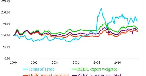
In this paper, we measure the real exchange rates by using International Monetary Fund (IMF) method and substitute the real commodity prices by terms of trade because of some calculation difficulties [8], [9].

Fig. 1. Dynamics of real commodity prices and real exchange rates.

Fig. 1 shows that the real exchange rates and terms of trade are move together over time besides the nominal exchange rates.

V. EMPIRICAL ANALYSIS

A. Economic Condition

In this section, we show the dynamics of foreign trade turnover, total exports, and total imports by following figures.

B. Empirical Results

1) Unit root test (ADF test)

According to result of Augmented Dickey-Fuller Unit root test, terms of trade, nominal exchange rates (export weighted, import weighted, and foreign trade weighted), and real exchange rates (export weighted, import weighted, and foreign trade weighted) are all I(1) process and these results are summarized in Table I [10], [11].

TABLEI:THE RESULT OF ADFTEST

Variables 0 order 1 order Integrated order

1. Terms of trade 0.187 0*** I(1)***

2. NEER, weighted by

foreign trade 0.195 0*** I(1)***

3. NEER, weighted by

exports 0.195 0*** I(1)***

4. NEER, weighted by _imports 0.227 0*** I(1)***

5. REER, weighted by

foreign trade 0.043** 0*** I(1)***

6. REER, weighted by _exports 0.096* 0*** I(1)***

7. REER, weighted by

imports 0.760 0*** I(1)***

Notes: (***), (**), (*) indicate probability to reject the null hypothesis that there is a unit root, with respectively 1, 5, 10 percent significance.

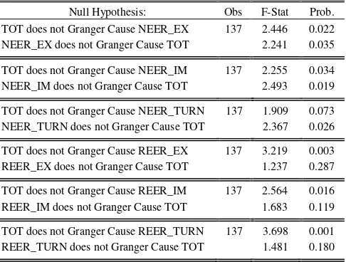
2) Granger causality test

As a result of Granger causality, terms of trade and nominal exchange rates have systematic relationships and terms of trade causes the real exchange rates (export weighted, import weighted, and foreign trade weighted).

TABLEII:PAIRWISE GRANGER CAUSALITY TESTS

Null Hypothesis: Obs F-Stat Prob. TOT does not Granger Cause NEER_EX 137 2.446 0.022 NEER_EX does not Granger Cause TOT 2.241 0.035

TOT does not Granger Cause NEER_IM 137 2.255 0.034 NEER_IM does not Granger Cause TOT 2.493 0.019 TOT does not Granger Cause NEER_TURN 137 1.909 0.073 NEER_TURN does not Granger Cause TOT 2.367 0.026 TOT does not Granger Cause REER_EX 137 3.219 0.003 REER_EX does not Granger Cause TOT 1.237 0.287 TOT does not Granger Cause REER_IM 137 2.564 0.016 REER_IM does not Granger Cause TOT 1.683 0.119 TOT does not Granger Cause REER_TURN 137 3.698 0.001 REER_TURN does not Granger Cause TOT 1.481 0.180

Mongolia is a small open economy country and it (real exchange rates) cannot influence to the world price (terms of trade). So it is impossible that real commodity prices and real exchange rates have systematic relationship. Thus, we conclude that there might be any relationship between the terms of trade and real exchange rates [12], [13].

3) Engle-granger co-integration test

We determine the long-run equilibrium relationship between real commodity prices and real exchange rates, based on Granger causality results [14].

The ADF test result suggests that residual series is stationary, which means there is any long-run relationship between the terms of trade and real exchange rates. By generalizing above results, error correction model is written as follows: t u EX REER TOT EX REER RESID EX REER 1 ) 1 ( _ 187 . 0 ) 2 ( 077 . 0 ) 1 ( _ _ 176 . 0 _              

 ₍₁₆₎

t u TURN REER TURN REER RESID TURN REER 2 ) 2 ( _ 165 . 0 ) 1 ( _ _ 217 . 0 _          

 ₍₁₇₎

t u IM REER TOT IM REER RESID IM REER 3 ) 1 ( _ 281 . 0 ) 2 ( 064 . 0 ) 1 ( _ _ 091 . 0 _              

 ₍₁₈₎

From error correction model, an increase in terms of trade appreciates the real exchange rate and average half-life of adjustment of real exchange rate is found to be about six months, five months, and 11 months for exchange rates weighted by exports, foreign trade, and imports, respectively.

4) Model stability and error analysis

We performed the error analysis of the error correction model by using Vensim software.

Fig. 3. Fanchart of the model of ToT and real exchange rates weighted by imports.

In Fig. 3, we can see the error correction model that indicates the relationship between real commodity price and real exchange rate is relatively stable.

VI. CONCLUSION

The exports of Mongolia have become largely dependent from mineral or primary products. Thus, this paper examines the Balassa-Samuelson hypothesis which an increase in price of primary goods appreciates the real exchange rates in case of Mongolia, based on monthly time series over the period 2000 to 2011.

For the data set we consider the terms of trade instead of real commodity prices and three kind of real exchange rates (weighted by exports, imports, and foreign trade) and we use Engle and Granger (1987) co-integration approach to assess whether the real exchange rates and real commodity prices move together over time.

As a result of empirical analysis, terms of trade is one of the factors that fluctuate the real exchange rate and average half-life of adjustment of real exchange rate is found to be about six months, five months, and 11 months for exchange rates weighted by exports, foreign trade, and imports,

Fanchart1 Estimation1 data

50% 75% 95% 100% dreerim 20 10 0 -10 -20

2000 2036 2073 2109 2145

Time (Year)

respectively.

Also, we check the stability of error correction model that indicates the short and long-run relationships between real commodity prices and real exchange rates by using Fanchart.

The main object of this paper was to examine whether there is any long-run relationships between two variables and in the further, it is interesting to develop the systematic model that can be implemented in policy decisions by determining other factors of real exchange rates.

ACKNOWLEDGMENT

The author is grateful to Purevjav Avralt-Od, doctoral student in University of Arizona, for outstanding guidance and stimulating discussions. Also, we address our thanks to Batsukh Tserendorj, Ph.D in economics, for his kindly and helpful comments.

REFERENCES

[1] P. Cashin, L. Cespedes, and R. Sahay, Keynes, Cocoa, and Copper: In search of Commodity Currencies, Washington: IMF, 2002.

[2] Y. C. Chen and K. Rogoff, Commodity Currencies and Empirical Exchange Rate Puzzles, Washington: IMF, 2002.

[3] L. F. Cespedes and A. Velasco, Macroeconomic Performance During Commodity Price Booms, Ankara: IMF, 2012.

[4] A. Harri, L. Nalley, and D. Hudson, “The Relationship between Oil, Exchange Rates, and Commodity Prices,”Journal of Agricultural and Applied Economics, vol. 41, no. 2, pp. 501-510, August 2009. [5] Y. Batzaya, “Relationship between Copper Price and Domestic

Currency, Togrog,” M.A. thesis, Dept. Econ., Institute of Finance and Economics, Ulaanbaatar, Mongolia, 2011.

[6] T. Koranchelian, The Equilibrium Real Exchange Rate in a Commodity Exporting Country: Algeria's Experience, Washington: IMF, 2005.

[7] R. F. Engle and C. W. J. Granger, “Co-Integration and Error Correction: Representation, Estimation, and Testing,”Econometrica, vol. 55, no. 2, pp. 251-276, Mar 1987.

[8] A. Zanello and D. Desruelle, A Primer on the IMF's Information Notice System, Washington: IMF, 1997.

[9] V. Q. Viet, A review of the Use of Price Index in National Accounts, Vientiane: United Nations Statistics Division, 2011.

[10] A. D. Schmidt, Pairs Trading: Cointegration Approach, Sydney: University of Sydney, 2008.

[11] S. Vuranok, Financial Development and Economic Growth: A Cointegration Approach, Ankara: Middle East Technical University,

2009.

[12] M. T. Bahadori and Y. Liu, “Granger causality analysis in irregular time series,” University of Southern California, 2012.

[13] S. Gelper, “Economic time series analysis: Granger causality and robustness,” Flanders: Katholieke Universiteit Leuven, 2008. [14] W. Enders, Applied econometrics time series, 1st ed., Ames: John

Wiley & Sons, Inc, 2000, ch. 6, pp. 373-377.

Tsenguunjav Byambasuren was born in Ulaanbaatar, Mongolia on 31th of May, 1991. An undergraduate student of Institute of Finance and Economics in Economics. His major field of study is general equilibrium, foreign trade, and monetary policy. And he did several researches in these fields.

He was working in Central bank of Mongolia, Mongolbank as an internship student twice. In 2012, he participated to the 15th _{International Students’} Conference of Ege University in Izmir, Turkey with the paper named “The policy analysis to improve mongolian foreign trade”. Furthermore, he was presenting his study in 8th _{International Student Conference that organized}

from Izmir University of Economics in 2012. He has been published following books and articles: Portfolio theory and performance analysis (Ulaanbaatar, Mongolia: Munkhiin useg, 2013; The policy analysis to improve mongolian foreign trade (Izmir, Tukey: Izmir University of Economics, 2012); Inflation targeting regime of monetary policy and its procyclical character (Ulaanbaatar, Mongolia: Mongolbank, 2011).