Comparison of Different Confidence Intervals of Intensities for an Open Queueing Network with Feedback

(1)

Comparison of Different Confidence Intervals of

Intensities for an Open Queueing Network

with Feedback

Vinayak Kawaduji Gedam

1

, Suresh Bajirao Pathare

2 1

Department of Statistics, University of Pune, Pune, India

2

Indira College of Commerce and Science, Pune, India Email: [email protected], [email protected]

Received March 14, 2012; revised April 30, 2012; accepted May 10, 2012

ABSTRACT

In this paper we propose a consistent and asymptotically normal estimator (CAN) of intensities



1

,



2

for a queueing

network with feedback (in which a job may return to previously visited nodes) with distribution-free inter-arrival and

service times. Using this estimator and its estimated variance, some

100 1









%

asymptotic confidence intervals of

intensities are constructed. Also bootstrap approaches such as Standard bootstrap, Bayesian bootstrap, Percentile

boot-strap and Bias-corrected and accelerated bootboot-strap are also applied to develop the confidence intervals of intensities. A

comparative analysis is conducted to demonstrate performances of the confidence intervals of intensities for a queueing

network with short run data.

Keywords:

Coverage Percentage; Relative Coverage; Bayesian Bootstrap; Bias-Corrected and Accelerated Bootstrap;

Percentile Bootstrap; Standard Bootstrap

1. Introduction

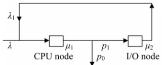
Consider a queueing network of a computer system with

feedback (in which a job may return to previously visited

nodes) as shown in

Figure 1

. This queueing network

con-sists of a CPU node and an Input/Output (I/O) node.

Ex-ternal jobs arrive at the CPU node according to the rate



. After service completion at CPU node, the job

pro-ceeds to the I/O node with probability p

1

, and with

prob-ability p

0

the job departs from the system, where

0

1

p

 

p

. Jobs leaving the I/O node are always fed back

to the CPU node (see

Figure 1

). The service times at each

node are with rates



1

and



2

respectively. The

suc-cessive service times at both nodes are assumed to be

mutually independent and independent of the state of the

system. The traffic intensity at the CPU node and I/O

node is given by

1

1 2

0 1 0 2

,

p









(1)

respectively. Intensity



1

and



2

can be interpreted as

expected number of arrivals per mean service time. The

condition for stability of the system is both



1

,



2

are

less unity.

Basic properties of queueing networks are introduced

in Disney [1]. Burke [2], Beautler and Melamed [3]

showed that the input process to a service center in a

network with feedback is not Poisson in general. It is for

this reason that Jacksons result is remarkable. Jacksons

[4] theorem states that each node behaves like an

inde-pendent queue.

(2)

[image:2.595.92.252.85.150.2]

Figure 1. An open queueing network with feedback.

developed by Buzen and Denning [11]. Efron [12-14] the

greatest statistician in the field of nonparametric

resam-pling approach, originally developed and proposed the

bootstrap, which is a resampling technique that can be

effectively applied to estimate the sampling distribution

of any statistic. Specifically, one can utilize the bootstrap

method to approximate the sampling distribution of a

statistic defined by a random sample from a population

with unknown probability distribution. And due to the

popularity of PC and statistical software, today the

boot-strap becomes the most powerful nonparametric

estima-tion procedure. Based upon the bootstrap resampling

technique, most statisticians utilize the standard bootstrap

(SB), percentile bootstrap (PB), and bias-corrected and

accelerated bootstrap (BCaB) approaches to produce

confidence intervals for practical problems.

Besides the standard bootstrap (SB) technique, Rubin

[15] presented the Bayesian bootstrap (BB) technique of

resampling. Miller [16] showed that the SB can be

re-garded as an extension of the jackknife. The BB is a

natural Bayesian analogue of the SB. The BB simulates

the posterior distribution of parameters under particular

model specifications, whereas the SB simulates the

esti-mated sampling distribution of a statistic estimating the

parameters. Both SB and BB can be applied to construct

confidence intervals of intensity for a queueing system

with distribution-free inter-arrival and service times.

Chu and Ke [17] constructed new confidence intervals

of mean response time for an M/G/1 FCFS queueing

system. Also, they performed the accuracy of bootstrap

confidence intervals through calculating the coverage

probability and the average length of confidence intervals.

Chu and Ke [18] proposed a consistent and

asymptoti-cally normal (CAN) estimator of the mean response time

for a G/M/1 queueing system, which is based on the

fixed point of empirical Laplace function. Ke and Chu

[19] proposed a consistent and asymptotically normal

estimator of intensity for a queueing system with

distri-bution-free interarrival and service times. Also, they

computed confidence intervals, testing statistical

hy-pothesis of intensity and power function associated with it

in this paper. Ke and Chu [20] constructed new

confi-dence intervals of intensity for a queueing system, which

are based on different bootstrap methods. They also

per-formed the accuracy of these bootstrap confidence

inter-vals through calculating the coverage probability and the

expected length of confidence intervals. They first

pro-posed bootstrapping technique and concept of relative

coverage to queueing system. They studied five

estima-tion approaches of intensity for a queueing system with

distribution free inter-arrival and service times for short

run. They have introduced a new measure called relative

coverage to assess the efficient performances of

confi-dence intervals.

In this paper we propose non parametric interval

esti-mation approach to intensities



1

,



2

for a open

queue-ing network with feedback. In Section 2 we prove that

the natural estimators



ˆ

1

,



ˆ

2

of intensities



1

and



2

are strongly consistent and asymptotically normal (CAN).

Based on the asymptotical normality of



ˆ

1

,



ˆ

2

, we can

construct a CAN confidence interval of



1

and



2

. Next

in Section 3 we establish the SB confidence interval of

1



,



2

via the standard bootstrap approach. In Section 4

we developed the derivation of the BB confidence

inter-val of



1

,



2

in terms of the Bayesian bootstrap

ap-proach. The percentile bootstrap (PB) confidence

inter-vals of



1

,



2

are developed in Section 5. In Section 6

we developed the bias-corrected and accelerated

boot-strap (BCaB) confidence intervals. A numerical

simula-tion study is conducted in Secsimula-tion 7 to demonstrate

per-formances of the interval estimation approaches for an

open queueing network with feedback using short run

data. All simulation results are shown by appropriate

tables for illustrating performances of the five interval

estimation approaches. Finally, we make some

conclu-sions in Section 8.

2. Nonparametric Statistical Inference of

Intensities

Let

X

1

and Y

1

be nonnegative random variables

repre-sents the inter-arrival and service time at CPU node.

Similarly

X

2

and Y

2

be nonnegative random variables

represents the inter-arrival and service time at I/O node

respectively. Given that a job just completed CPU node

burst, it will next request I/O node service with probability

1

p

and with probability

p

0

, where

p

0

 

1 p

1

departs

from the system. The random variables at CPU node and

I/O node are independent. The intensities are defined as

follows:

1 1

0 1

Y

X

p









and

2

0 2

1

Y

X

p









, (2)

where



X₁

,



X2

denote the mean inter-arrival times at

CPU node and I/O node respectively. Similarly



Y₁

,



Y2

denote the mean service times at CPU node and I/O node

respectively. Equation (2) is equivalent to Equation (1).

2.1. Estimating Intensities

(3)

from

X

1

and

p Y p Y

0 11

,

0 12

,



,

p Y

0 1n

is a random sample

drawn from Y

1

. Let



X

1i

,

p Y

0 1i



represents inter-arrival

time and service time for the i

th

_{customer of CPU node.}

Similarly assume

p X

1 21

,

p X

1 22

,



,

p X

1 2m

is a random

sample drawn from X

2

and

p Y

0 21

,

p Y

0 22

,



,

p Y

0 2m

is a

random sample drawn from Y

2

. Let



p X

1 2i

,

p Y

0 2i



represents inter-arrival time and service time for the i

th

customer of I/O node.

Let

X X Y Y

1

,

2

,

1

,

2

be the sample means of X

1

, X

2

, Y

1

,

Y

2

respectively.

1 1 2 1 2

1 1

1 0 1 2 0 2

1 1

1

1 ,

1

1 ,

n m i i i i n m i i i i

X

p X

n

m

Y

p Y Y

p Y

n

m

   





According to the Strong Law of Large Numbers, we

know that

X X Y Y

1

,

2

,

1

,

2

are strongly consistent

estima-tor of

1

,

2

,

1

,

2

X X Y Y



 

respectively. Thus a strongly

consistent estimator of intensities are given by

1 2

ˆ

Y

,

ˆ

Y

X









(3)

In practical queueing network, the true distributions of

X

1

, X

2

,

Y

1

, Y

2

are rarely known, so the exact distributions

of

 

ˆ

1

,

ˆ

2

cannot be derived. But under the assumption

that X

1

and Y

1

,

X

2

and Y

2

being independent, the

asymp-totic distributions of

 

ˆ

1

,

ˆ

2

can be developed by the

following procedures.

Firstly, according to the Central Limit Theorem (see

[21] p. 234), we have











11





11



2 1 2 1 0

0,

and

0,

D X X D Y Y

n X

N

n Y

p

N

















(4)

where

1

2

X



and

1

2

Y



are variances of X

1

and Y

1

,

respec-tively.

Also,











2



2



2



2

2 2 1 2 2 0

0,

and

0,

,

D X X D Y Y

m X

p

N

m Y

p

N

















(5)

where

2

X



and

2

Y



are variances of X

2

and Y

2

,

re-spectively, and



D

denotes convergence in

distribu-tion.

Next note that













1 1

1 1 1 1

1

1 1 0 1

1

1 0 0 1

1

ˆ

.

Y

X

X Y Y X

X

n

p

Y

n

X

n

Y

p

X

 













_





_

















Also,













2 2

2 2 2 2

2

2 2 0 2

2 1

1 2 0 0 2 1

1 2

ˆ

.

Y

X

X Y Y X

X

m

p

Y

m

X

p

m p

Y

p

X

p

X















_





_







_









(6)

Therefore by the Slutsky’s theorem [see [21] p. 227],

we get







2



1 1 1

ˆ

D

0,

n

 





N



,

where

1 1 1 1

1

2 2 2 2 2

0 2

1 4

X Y Y X X

p

 









.

And







2



2 2 2

ˆ

D

0,

m









N



(7)

where

2 2 2 2

2

2 2 2 2 2 2

1 0

2

2 2 4

1

X Y Y X X

p

 









.

Now, set

1 1 2 2

2 2 2 2 2

1 0 1

2

1 4

1

2 2 2 2 2 2

1 2 0 2

2

2 2 4

1 2

ˆ

and

ˆ

,

Y X

X S

p Y S

X

p X S

p Y S

p X











(8)

where

















1 1 2 2 2 2 2 2

1 1 0 1 1

1 1

2 2

1 2 2 0 2 2

1 1

1

1 ,

1

1 and

.

n n

X i Y i

i i

m m

X i Y i

i i

S

X

S

p Y

Y

n

S

p X

X

S

p Y

Y

m

   



















Then

 

ˆ

12

,

ˆ

22

are strongly consistent estimators of

2 2

1

,

2

 

respectively. Applying the Slutsky’s theorem

once again, we deduce that





_{ }





_{ }

1 1 1 2 2 2

ˆ

0,1 and

ˆ

0,1

ˆ

D D

n

N

m

N

 















(9)

Thus

 

ˆ

1

,

ˆ

2

are strongly consistent and

asymptoti-cally normal (CAN) estimators with approximate vari-

ances

2 2 1 2

ˆ

,

n

m

 

respectively.

2.2. Confidence Intervals

Using the CAN estimators

 

ˆ

1

,

ˆ

2

and its associated

approximate variances

2 2 1 2

ˆ

,

n

m

 

(4)

dence intervals of intensities



1

&



2

for a open

queue-ing network with feedback. Let

z

_

be the upper



th

quantile of the standard normal distribution, by the as-

ymptotic distribution of



1 1





2 2



1 2

ˆ

&

ˆ

n

 

m







in expression (9), an approximate

100 1









%

confi-dence interval of



1

&



2

are obtained as



1 1



2 2

1

2 1 2 1

1 1 1

ˆ

1 ˆ

ˆ

n

P

z

P

n

   

 













 



_







_











_







_





Consequently, an approximate

100 1









%

confi-dence interval of



1

is

2 1 2 1

1 1

ˆ

z

,

ˆ

z

n



























. (10)

Similarly, an approximate

100 1









%

confidence

interval of



2

is

2 2 2 2

2 2

ˆ

z

,

ˆ

z

m



























. (11)

3. Standard Bootstrap Confidence Intervals

of Intensities

Now the bootstrap confidence intervals are developed as

follows:

Let

x x

11

,

12

,



,

x

1n

be a random sample of n

observa-tions taken from the population X

1

and

p y p y

0 11

,

0 12

,



,

0 1n

p y

be a random sample of n observations taken from

the population Y

1

. According to the bootstrap procedure,

a simple random sample

x x

11

,

12

,

x

1n

 

_



can be taken

from the empirical distribution function of

x x

11

,

12

,



,

x

1n

called a bootstrap sample from

x x

11

,

12

,



,

x

1n

. Also, we

can draw a bootstrap sample

p y p y

0 11

,

0 12

,

p y

0 1n

 

_



from

0 11

,

0 12

,

0 1n

p y



p y

. It follows from Equation (2) that

an estimate of intensity



1

can be calculated from

boot-strap samples as

1 1 1

ˆ

y

x



  



, (12)

where

x

1 

and

y

1 

are the sample means of

x x

11

,

12

,

 

_

1n

x



and

p y

0 11

,

p y

0 12

,

p y

0 1n

 

_



respectively and



ˆ

1 

is

called a bootstrap estimate of



1

. The above resampling

process can be repeated N

1

times. The N

1

bootstrap

esti-mates

 

ˆ

11

,

ˆ

12

,



ˆ

1N₁

 

_



can be computed from the

boot-strap resamples. Averaging the N

1

bootstrap estimates we

obtain that

1 1 1 1 1

1 ˆ

ˆ

N N i i

N



 





(13)

is the bootstrap estimate of



1

. And the standard

devia-tion of



ˆ

1

can be estimated by

 

1





1 1 1 2 2 1 1 1

1 ˆ

ˆ

.

1

N

N i N

i

sd

N

















_











(14)

Because the central limit theorem implies that the

dis-tribution of



ˆ

1

is approximately normal. A

100 1









%

SB confidence interval for



1

is

 





ˆ

1



z sd

2



ˆ

N1

,



ˆ

1



z sd

2



ˆ

N1



,

(15)

Similarly

p x

1 21

,

p x

1 22

,



,

p x

1 2m

is a random sample

of m observation drawn from population X

2

and

p y

0 21

,

0 22

,

0 2m

p y



p y

is a sample of m observations taken

from the population

Y

2

. According to the bootstrap

pro-cedure, a simple random sample

p x

1 21

,

p x

1 22

,

p x

1 2m

 

_



can be taken from the empirical distribution function of

1 21

,

1 22

,

1 2m

p x



p x

called a bootstrap sample from

1 21

,

1 22

,

1 2m

p x



p x

. Also, we can draw a bootstrap

sample

p y

0 21

,

p y

0 22

,

p y

0 2m

 

_



from

p y

0 21

,

p y

0 22

,



,

0 2m

p y

. An estimate of intensity



2

can be calculated

from bootstrap samples as

2 2 2

ˆ

y

x



  



, (16)

where

x

2 

and

y

2 

are the sample means of

p x

1 21

,



1 22

,

1 2m

p x



_

p x



and

p y

0 21

,

p y

0 22

,



,

p y

0 2m

respec-tively and



ˆ

2 

is called a bootstrap estimate of



2

. The

above resampling process can be repeated M

1

times. The

M

1

bootstrap estimates

 

ˆ

21

,

ˆ

22

,



,



ˆ

2M₁

can be

com-puted from the bootstrap resamples. Averaging the M

1

bootstrap estimates we obtain that

1 1 2 1 1

1 ˆ

ˆ

M M i i

M



 





(17)

is the bootstrap estimate of



2

. And the standard

devia-tion of



ˆ

2

can be estimated by

 

1



1



1 2 2 2 1 1

1 ˆ

ˆ

.

1

M

M i M

i

sd

M















_



_









(18)

Because the central limit theorem implies that the

dis-tribution of



ˆ

2

is approximately normal. A

100 1









%

SB confidence interval for



2

is

 





ˆ

2



z sd

2



ˆ

M1

,



ˆ

2



z sd

2



ˆ

M1



,

(19)

4. Bayesian Bootstrap Confidence Intervals

of Intensities

The Bayesian bootstrap is analogous to the standard

bootstrap. Each BB replication generates a posterior

probability for each

x

1i

. Specifically, one BB replication

(5)

 n

1 r



. Then

w

1i





w w

11

,

12

,



,

w

1n



is the vector of

probabilities attached to the inter-arrival data values

11

,

12

,

1n

x x



x

in that BB replication. Considering all BB

replications gives the BB distribution of the distribution

of

X

1

and thus of any parameter of this distribution.

Hence for



X₁

(the mean of X

1

), in each BB replication

we calculate



X₁

as if

w

1i

were the probability that

1 i

X



x

that is, we calculate

1 1 1 1

n i i i

x



w x





. The dis-

tribution of the values of

x

1 

overall BB replications is

the BB distribution of

1

X



.

Also, generating a vector of probabilities





1 11

,

12

,

1n

v



v v



v

attached to the service time data

values

p y

0 11

,

p y

0 12

,



,

p y

0 1n

in a BB replication, and we

calculate

1 0 1 1 1

n i i i

y



p

v y





for

1

Y



(the mean of Y

1

).

Then in terms of equation (2) an estimate of intensity



1

can be calculated from BB replications as

1 1 1

ˆ

y

x



  



, (20)

where



ˆ

1 

is called a Bayesian bootstrap estimate of

1



. The above BB process can be repeated N

1

times. The

N

1

BB estimates,

 

ˆ

11

,

ˆ

12

,



ˆ

1N₁

 

_



can be computed

from the BB replications. Averaging the N

1

BB estimates,

we obtain that

1 1 1 1

1 ˆ

ˆ

N BB j j

N



 

 



, (21)

is the BB estimate of



1

. And the standard deviation of

1

ˆ



can be estimated by





1





1 2 2 1 BB 1 1

1 ˆ

ˆ

1

N BB j j

sd

N

















_





_









. (22)

Applying the asymptotical normality of



ˆ

1

, a





100 1





%

BB confidence interval for



1

is













ˆ

1



z sd

2



ˆ

BB



,



ˆ

1



z sd

2



ˆ

BB





. (23)

Similarly each BB replication generates a posterior

probability for each

x

2i

. Specifically, one BB

replica-tion is generated by drawing

m



1 uniform

 

0,1

ran-dom numbers

r r

1

, ,

2



,

r

m1

, ordering them and

calculat-ing the gaps

w

2i



r

_{ }i



r

_{ }i1

,

i



1, 2,



,

m

, where

r

 0



0 and

r

_{ }_m



1 . Then

w

2i





w w

21

,

22

,



,

w

2m



is the

vec-tor of probabilities attached to the inter-arrival data

val-ues

p x

1 21

,

p x

1 22

,



,

p x

1 2m

in that BB replication.

Con-sidering all BB replications gives the BB distribution of

the distribution of X

2

and thus of any parameter of this

distribution. Hence for



X₂

(the mean of X

2

), in each

BB replication we calculate



X₂

as if

w

2i

were the

probability that

X

2



x

2i

that is, we calculate

2 1 2 2

1

m i i i

x



p

w x





. The distribution of the values of

x

2 

over all BB replications is the BB distribution of



X₂

.

Also, generating a vector of probabilities





2 21

,

22

,

2m

v



v v



v

attached to the service time data

values

p y

0 21

,

p y

0 22

,



,

p y

0 2m

in a BB replication, and

we calculate

2 0 2 2 1

m i i i

y



p

v y





for



Y₂

(the mean of

Y

2

).

Then in terms of Equation (2) an estimate of intensity

2



can be calculated from BB replications as

2 2 2

ˆ

y

x



  



, (24)

where



ˆ

2 

is called a Bayesian bootstrap estimate of

2



. The above BB process can be repeated M

1

times.

The

M

1

BB estimates,

 

ˆ

21

,

ˆ

22

,



ˆ

2M₁

 

_



can be

com-puted from the BB replications. Averaging the M

1

BB

estimates, we obtain that

1 2 1 1

1 ˆ

ˆ

M BB j j

M



 

 

_

, (25)

is the BB estimate of



2

. And the standard deviation of

2

ˆ



can be estimated by





1





2

2 1 1

1 ˆ

ˆ

1

M

BB j BB

j

sd

M

















_





_









. (26)

Applying the asymptotical normality of



ˆ

2

, a





100 1





%

BB confidence interval for



2

is













ˆ

2



z sd

2



ˆ

BB



,



ˆ

2



z sd

2



ˆ

BB





(27)

5. Percentile Bootstrap Confidence Intervals

of Intensities

Let

1

11 12 1

ˆ

,

ˆ

,

ˆ

_N

 

 

_





and

1

21 22 2

ˆ

,

ˆ

,

ˆ

_M

 

 

_





call the

boot-strap distribution of

 

ˆ

1

,

ˆ

2

respectively. Let



ˆ 1

1

 



,

 

1 1 1

ˆ

2 ,

,

ˆ

N





_





and



ˆ

2

 

1 ,



ˆ

2

 

2 ,

,



ˆ

2

 

M

1

 

_



be

order statistics of

1

11 12 1

ˆ

,

ˆ

,

ˆ

N

 

 

_





and

1

21 22 2

ˆ

,

ˆ

,

ˆ

_M

 

 

_





respectively. Then utilizing the

100 



2 th



and





100 1





2 th

percentage points of the bootstrap

dis-tribution, a

100 1









%

PB confidence interval for



1

,

2



are obtained as

1 1 1 1

ˆ

,

ˆ

1 ,

2

2 N



N















 











_











 



















_

_

_{ }

_

_

_

_

_

_

_

_







(28)

2 1 2 1

ˆ

,

ˆ

1 ,

2

2 M



M















 











_











 



















_

_

_{ }

_

_

_

_

_

_

_

_







(29)

where [x] denotes the greatest integer less than or equal

to x.

6. Bias-Corrected and Accelerated Bootstrap

Confidence Intervals of Intensities

The bootstrap distribution

1

11 12 1

ˆ

,

ˆ

,

ˆ

_N

 

 

_





(6)

1

22 2

ˆ

,

ˆ

_M





_





may be biased. This method is designed to

correct this potential bias of the bootstrap designed. Set





1 ₁ ₁

1 1

ˆ

N j j

I

p

N











 

_

and





1 ₂ ₂

1 1

ˆ

M j j

I

p

M











 

_

,

where

I

 



is the indicator function. Define

z

ˆ

0



1

 

p



_



and

1

 

1

ˆ

z

_





p

_

, where



1

denotes the inverse

func-tion of the standard normal distribufunc-tion



. Except for

correcting the potential bias of the bootstrap distribution,

we can accelerate convergence of bootstrap distribution.

Let

X i



1

 

and

p Y i

0 1



 

denote the original samples

with the i

th

_{observation x}

1i

and

p y

0 1i

deleted, also let

1

ˆ

_i



be the estimator of



1

calculated by using

X i



1

 

and

p Y i

0 1



 

Define

1 1

1

1 ˆ

n i i

n









, Similarly

p X i

1



2

 

,

 

0 2

p Y i



denote the original samples with the i

th

obser-vation

p x

1 2i

and

p y

0 2i

deleted, also



ˆ

2i

be the

esti-mator of



2

calculated by using

p X i

1



2

 

and

p Y i

0 2



 

.

Define

2 2

1

1 ˆ

m i i

m









And









 









 

3 2 3 2 3 1 1 1 1 2 1 1 1 3 2 2 1 2 2 2 2 1

ˆ

,

ˆ

6 ˆ

ˆ

6

n i i n i i m i i m i i

a

 



   







_

_





_



























_

_





_







_



_













(30)

where

z z a

ˆ

0

,

ˆ

1

,

ˆ

1

, and

a

ˆ

2

are named bias-correction and

acceleration respectively.

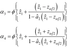
Thus a

100 1









%

Bias-corrected and accelerated

bootstrap (BCaB) Confidence Interval of intensities



1

,

2



are constructed by





















ˆ

1

N

1



1

,



ˆ

1

N

1



2



 

(31)





















ˆ

2

M

1



3

,



ˆ

2

M

1



4



 

(32)

where









0 2 1 0

1 0 2

ˆ

1 z

z

a z

z

 

 



































0 2 2 0

1 0 2

ˆ

1 z

z

a z

z

 











_







_



















1 2 3 1

2 1 2

ˆ

1 z

z

a z

z

 







































1 2 4 1

2 1 2

ˆ

1 z

z

a z

z

 































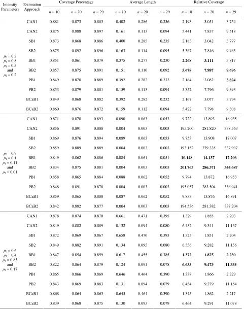
7. Simulation Study

To evaluate performances of the different interval

esti-mation approaches mentioned above for an open

queue-ing network with feedback usqueue-ing short run data, a

nu-merical simulation study was undertaken. Most of the

statisticians assess performances of interval estimations

in terms of coverage percentages or average lengths of

confidence intervals. However, through simulation study

in the research work, we find that larger coverage

per-centages of confidence interval may often be due to

wider standard deviation of interval estimation methods.

Moreover, narrower confidence intervals may often lead

to smaller coverage percentages. Hence, both coverage

percentage and average length are not efficient for

ap-praising interval estimation methods. In order to

over-come above two shortcomings, we propose a measure

called relative coverage to evaluate performances of

in-terval estimation methods where,

Coverage percentage

Relative coverage

Average length



.

The larger of the relative coverage implies the better

performance of the corresponding confidence interval. In

order to reach this goal, we set a continuous distribution

with mean

1 

on inter-arrival time X

1

and X

2

. Also set

continuous distribution with mean

1 

1

on the service

time

Y

1

at CPU node and continuous distribution with

mean

1 

2

on the service time Y

2

at I/O node. The

lev-els of p

0

considered in the simulation study are 0.1 to 0.9

where as levels of p

1

are 0.9 to 0.1, where p

0

is the

prob-ability that the job departs from the system and p

1

is the

probability that after service completion at CPU node, the

job proceeds to the I/O node. This means with probability

0

0.1 p



the job departs from the system and with

probability

p

1



0.9 , after service completion at CPU

node, the job proceeds to the I/O node and so on. Also we

have considered the values of



1

and



2

such that

1

[image:6.595.364.480.84.167.2] [image:6.595.58.288.168.501.2]





and



2



1 for simulation study. Note that in

Table 1

wherever



1



1 and



2



1 such values of

1



and



2

are not considered for simulation study.

The intensity parameters



1

and



2

are calculated

using Equation (1). The different values of



,

µ

1

,

µ

2

,

p

0

and p

1

are considered for simulation study as shown in

Table 1

.

(7)

Table 1. Different levels of intensity parameters considered in the simulation study.

λ = 0.1, µ1 = 1, µ2 = 1 λ = 0.1, µ1 = 1, µ2 = 2 λ = 0.1, µ1 = 2, µ2 = 1

p0 p1 ρ1 ρ2 p0 p1 ρ1 ρ2 p0 p1 ρ1 ρ2

0.1 0.9 1 0.9 0.1 0.9 1 0.45 0.1 0.9 0.5 0.9

0.2 0.8 0.5 0.4 0.2 0.8 0.5 0.2 0.2 0.8 0.25 0.4

0.3 0.7 0.33 0.23 0.3 0.7 0.33 0.12 0.3 0.7 0.17 0.23

0.4 0.6 0.25 0.15 0.4 0.6 0.25 0.08 0.4 0.6 0.13 0.15

0.5 0.5 0.2 0.1 0.5 0.5 0.2 0.05 0.5 0.5 0.1 0.1

0.6 0.4 0.17 0.07 0.6 0.4 0.17 0.03 0.6 0.4 0.08 0.07

0.7 0.3 0.14 0.04 0.7 0.3 0.14 0.02 0.7 0.3 0.07 0.04

0.8 0.2 0.13 0.03 0.8 0.2 0.13 0.01 0.8 0.2 0.06 0.03

0.9 0.1 0.11 0.01 0.9 0.1 0.11 0.01 0.9 0.1 0.06 0.01

λ = 0.5, µ1 = 1, µ2 = 1 λ = 0.5, µ1 = 1, µ2 = 2 λ = 0.5, µ1 = 2, µ2 = 1

p0 p1 ρ1 ρ2 p0 p1 ρ1 ρ2 p0 p1 ρ1 ρ2

0.1 0.9 5 4.5 0.1 0.9 5 2.25 0.1 0.9 2.5 4.5

0.2 0.8 2.5 2 0.2 0.8 2.5 1 0.2 0.8 1.25 2

0.3 0.7 1.67 1.17 0.3 0.7 1.67 0.58 0.3 0.7 0.83 1.17

0.4 0.6 1.25 0.75 0.4 0.6 1.25 0.38 0.4 0.6 0.63 0.75

0.5 0.5 1 0.5 0.5 0.5 1 0.25 0.5 0.5 0.5 0.5

0.6 0.4 0.83 0.33 0.6 0.4 0.83 0.17 0.6 0.4 0.42 0.33

0.7 0.3 0.71 0.21 0.7 0.3 0.71 0.11 0.7 0.3 0.36 0.21

0.8 0.2 0.63 0.13 0.8 0.2 0.63 0.06 0.8 0.2 0.31 0.13

0.9 0.1 0.56 0.06 0.9 0.1 0.56 0.03 0.9 0.1 0.28 0.06

λ = 0.9, µ1 = 1, µ2 = 1 λ = 0.9, µ1 = 1, µ2 = 2 λ = 0.9, µ1 = 2, µ2 = 1

p0 p1 ρ1 ρ2 p0 p1 ρ1 ρ2 p0 p1 ρ1 ρ2

0.1 0.9 9 8.1 0.1 0.9 9 4.05 0.1 0.9 4.5 8.1

0.2 0.8 4.5 3.6 0.2 0.8 4.5 1.8 0.2 0.8 2.25 3.6

0.3 0.7 3 2.1 0.3 0.7 3 1.05 0.3 0.7 1.5 2.1

0.4 0.6 2.25 1.35 0.4 0.6 2.25 0.68 0.4 0.6 1.13 1.35

0.5 0.5 1.8 0.9 0.5 0.5 1.8 0.45 0.5 0.5 0.9 0.9

0.6 0.4 1.5 0.6 0.6 0.4 1.5 0.3 0.6 0.4 0.75 0.6

0.7 0.3 1.29 0.39 0.7 0.3 1.29 0.19 0.7 0.3 0.64 0.39

0.8 0.2 1.13 0.23 0.8 0.2 1.13 0.11 0.8 0.2 0.56 0.23

0.9 0.1 1 0.1 0.9 0.1 1 0.05 0.9 0.1 0.5 0.1

(8)

0 12

,

0 1n

p Y



p Y

are drawn from X

1

and Y

1

respectively.

Also for each level of



2

random samples of inter-ar-

rival times

p X

1 21

,

p X

1 22

,



,

p X

1 2m

and service times

0 21

,

0 22

,

0 2m

p Y



p Y

are drawn from X

2

and Y

2

respec-tively. Next N = 1000 bootstrap resamples each of size n

and m = 10, 20, 29 are drawn from the original samples,

as well as N = 1000 BB replications are simulated for the

original samples. According to Equations (10), (11), (15),

(19), (23), (27)-(29), (31) and (32) in respective, we

ob-tain CAN1, CAN2, SB1, SB2, BB1, BB2, PB1, PB2,

BCaB1 and BCaB2 confidence intervals of intensities



1

and



2

with confidence level 90%. The above

simula-tion process is replicated N

= 1000 times and we

com-pute coverage percentages, average lengths and relative

coverage of the above mentioned confidence intervals.

We utilize a PC Dual Core and apply Matlab

®

7.0.1 to

accomplish all simulations.

Here

M represents exponential distribution, E

4

a 4-

stage Erlang distribution,

4

Pe

H

a 4-stage hyper-expo-

nential distribution and

4

Po

H

a 4-stage hypo-exponen-

tial distribution.

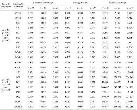
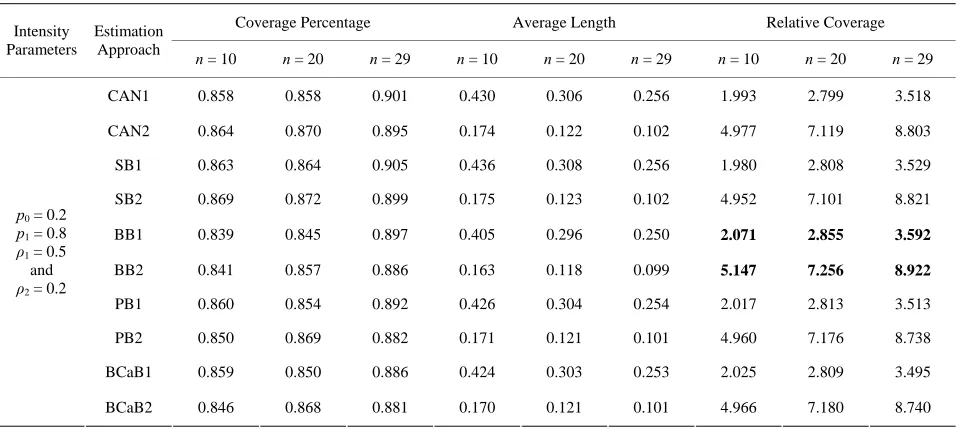
Based on the above mentioned interval estimation

ap-proaches, the coverage percentage, average lengths and

relative coverage of intensities



1

and



2

are shown in

[image:8.595.312.537.210.313.2]

Tables 3

to

7 for queueing network models (presented in

Table 2

) with short run data, we find that average lengths

Table 2. Different queueing network models simulated for study.

Queueing Networks Models Simulated

41

M E to E M4 1

1

M G to G M 1

4 1

Pe

M H to 4 1

Pe

H M

4 4 1

Pe

E H to 4 41

Pe

H E

4 4 1

Po

E H to 4 4 1

Po

H E

1

G G to G G1

4 4 1

Pe Po

H H to 4 4 1

Po Pe

[image:8.595.59.540.356.735.2]

H H

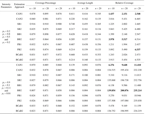
Table 3. Simulation results of coverage percentage, average lengths, and relative coverage for 90% confidence intervals un-der queueing network. M E₄ 1 to E₄ M 1.

Coverage Percentage Average Length Relative Coverage Intensity

Parameters

Estimation Approach _n

= 10 n = 20 n = 29 n = 10 n = 20 n = 29 n = 10 n = 20 n = 29 CAN1 0.878 0.895 0.878 0.611 0.416 0.345 1.437 2.151 2.548

CAN2 0.840 0.881 0.871 0.220 0.162 0.135 3.816 5.431 6.465 SB1 0.916 0.910 0.900 0.748 0.455 0.365 1.225 2.002 2.465 SB2 0.835 0.875 0.869 0.217 0.161 0.134 3.843 5.425 6.480 BB1 0.879 0.898 0.877 0.628 0.418 0.344 1.399 2.148 2.547 BB2 0.817 0.864 0.856 0.205 0.157 0.131 3.978 5.517 6.514 PB1 0.832 0.874 0.867 0.687 0.438 0.356 1.211 1.994 2.437 PB2 0.831 0.874 0.869 0.214 0.159 0.133 3.892 5.490 6.537

BCaB1 0.831 0.877 0.872 0.668 0.433 0.353 1.243 2.026 2.473

p0 = 0.2

p1 = 0.8

ρ1 = 0.5

and

ρ2 = 0.2

BCaB2 0.837 0.871 0.871 0.214 0.160 0.133 3.913 5.454 6.535 CAN1 0.870 0.885 0.868 0.139 0.092 0.076 6.276 9.648 11.410

CAN2 0.832 0.878 0.867 0.006 0.004 0.004 134.515 195.434 232.230 SB1 0.910 0.912 0.887 0.171 0.100 0.081 5.310 9.116 11.013 SB2 0.827 0.879 0.866 0.006 0.004 0.004 135.068 196.738 232.756 BB1 0.879 0.882 0.867 0.143 0.092 0.076 6.138 9.586 11.400 BB2 0.807 0.871 0.858 0.006 0.004 0.004 139.854 200.876 235.214

PB1 0.824 0.871 0.859 0.156 0.096 0.078 5.270 9.031 10.946 PB2 0.826 0.869 0.866 0.006 0.004 0.004 137.508 197.084 235.030 BCaB1 0.833 0.872 0.868 0.152 0.095 0.078 5.478 9.169 11.159

p0 = 0.9

p1 = 0.1

ρ1 = 0.11

and

ρ2 = 0.01

(9)

Continued

CAN1 0.851 0.876 0.866 1.012 0.697 0.579 0.841 1.258 1.496

CAN2 0.829 0.891 0.891 0.186 0.135 0.112 4.459 6.600 7.935

SB1 0.893 0.894 0.882 1.249 0.760 0.613 0.715 1.176 1.438

SB2 0.826 0.890 0.887 0.184 0.134 0.112 4.492 6.631 7.925

BB1 0.856 0.879 0.865 1.045 0.700 0.578 0.819 1.256 1.496

BB2 0.814 0.886 0.878 0.173 0.131 0.110 4.693 6.783 8.010

PB1 0.827 0.866 0.848 1.135 0.732 0.598 0.729 1.184 1.418

PB2 0.830 0.884 0.886 0.181 0.132 0.111 4.595 6.673 7.993

BCaB1 0.827 0.866 0.848 1.108 0.722 0.593 0.747 1.199 1.431

p0 = 0.6

p1 = 0.4

ρ1 = 0.83

and

ρ2 = 0.17

BCaB2 0.824 0.883 0.881 0.181 0.133 0.111 4.553 6.636 7.934

CAN1 0.882 0.891 0.879 0.682 0.470 0.384 1.293 1.895 2.286

CAN2 0.859 0.861 0.875 0.031 0.022 0.019 27.501 38.453 46.779

SB1 0.915 0.912 0.893 0.841 0.515 0.408 1.088 1.771 2.189

SB2 0.850 0.858 0.873 0.031 0.022 0.019 27.505 38.524 46.903

BB1 0.889 0.892 0.878 0.704 0.472 0.385 1.262 1.889 2.283

BB2 0.831 0.850 0.867 0.029 0.022 0.018 28.516 39.337 47.492

PB1 0.847 0.861 0.852 0.767 0.496 0.397 1.104 1.737 2.144

PB2 0.850 0.848 0.877 0.030 0.022 0.018 28.019 38.473 47.602

BCaB1 0.846 0.856 0.852 0.746 0.490 0.394 1.133 1.749 2.163

p0 = 0.9

p1 = 0.1

ρ1 = 0.56

and

ρ2 = 0.03

BCaB2 0.857 0.850 0.877 0.030 0.022 0.018 28.158 38.438 47.496

CAN1 0.842 0.893 0.880 0.588 0.418 0.342 1.431 2.138 2.570

CAN2 0.842 0.856 0.879 1.016 0.730 0.618 0.829 1.173 1.423

SB1 0.894 0.909 0.899 0.716 0.456 0.362 1.249 1.993 2.481

SB2 0.839 0.856 0.877 1.005 0.725 0.615 0.835 1.181 1.425

BB1 0.850 0.890 0.875 0.605 0.420 0.342 1.406 2.119 2.560

BB2 0.830 0.847 0.874 0.948 0.705 0.603 0.875 1.201 1.449

PB1 0.810 0.866 0.874 0.658 0.439 0.353 1.230 1.972 2.475

PB2 0.834 0.846 0.870 0.986 0.717 0.610 0.846 1.180 1.427

BCaB1 0.810 0.865 0.875 0.639 0.433 0.349 1.267 1.998 2.504

p0 = 0.1

p1 = 0.9

ρ1 = 0.5

and

ρ2 = 0.9

(10)

Continued

CAN1 0.841 0.868 0.878 0.764 0.523 0.431 1.101 1.659 2.037

CAN2 0.851 0.863 0.875 0.837 0.600 0.505 1.016 1.439 1.732 SB1 0.891 0.888 0.890 0.944 0.572 0.455 0.944 1.552 1.955 SB2 0.850 0.859 0.875 0.828 0.596 0.503 1.026 1.440 1.739 BB1 0.849 0.871 0.873 0.790 0.526 0.431 1.075 1.657 2.025 BB2 0.832 0.849 0.864 0.781 0.580 0.494 1.066 1.465 1.748 PB1 0.810 0.849 0.863 0.864 0.551 0.444 0.937 1.540 1.943 PB2 0.843 0.854 0.881 0.813 0.589 0.498 1.037 1.449 1.767

BCaB1 0.817 0.853 0.862 0.840 0.544 0.441 0.973 1.569 1.957

p0 = 0.4

p1 = 0.6

ρ1 = 0.63

and

ρ2 = 0.75

BCaB2 0.841 0.854 0.869 0.814 0.592 0.499 1.033 1.443 1.740

CAN1 0.853 0.887 0.896 0.334 0.231 0.193 2.554 3.841 4.639 CAN2 0.831 0.873 0.862 0.063 0.045 0.037 13.279 19.278 23.249

SB1 0.893 0.906 0.911 0.411 0.251 0.205 2.171 3.611 4.452 SB2 0.828 0.869 0.859 0.062 0.045 0.037 13.405 19.311 23.232 BB1 0.856 0.890 0.897 0.345 0.232 0.193 2.484 3.844 4.645

BB2 0.815 0.861 0.861 0.058 0.044 0.036 13.972 19.708 23.773

PB1 0.824 0.858 0.877 0.377 0.242 0.199 2.187 3.546 4.398 PB2 0.838 0.872 0.861 0.061 0.044 0.037 13.825 19.620 23.521 BCaB1 0.830 0.857 0.880 0.364 0.238 0.198 2.278 3.595 4.449

p0 = 0.9

p1 = 0.1

ρ1 = 0.28

and

ρ2 = 0.06

BCaB2 0.837 0.873 0.862 0.061 0.045 0.037 13.803 19.574 23.512

[image:10.595.60.538.522.734.2]

Note that: 1) boldface denotes the greatest relative coverage among the five estimation approach; 2) Confidence intervals of ρ1 under different estimation ap-proaches are denoted by CAN1, SB1, BB1, PB1 and BCaB1; 3) Confidence intervals of ρ2 under different estimation approaches are denoted by CAN2, SB2, BB2, PB2 and BCaB2.

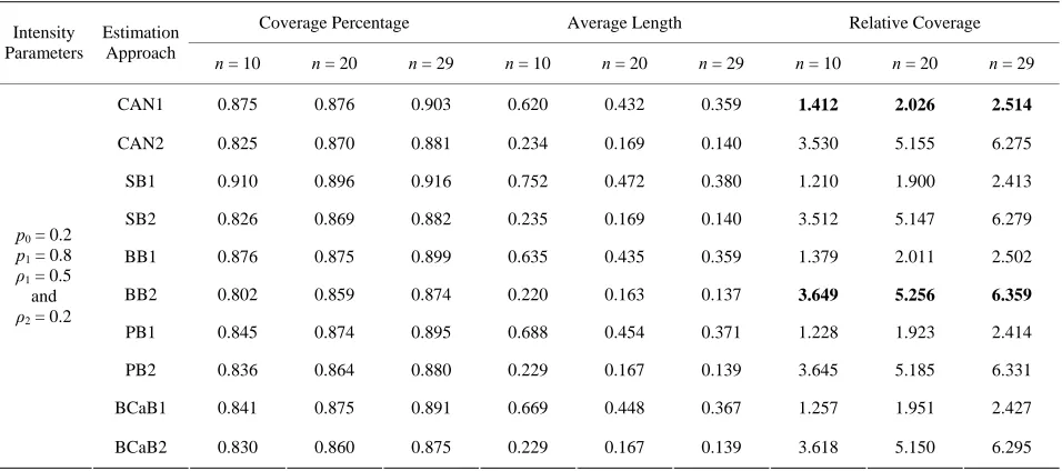
Table 4. Simulation results of coverage percentage, average lengths, and relative coverage for 90% confidence intervals un-der queueing network. ₄Pe 1

M H to ₄Pe 1

H M .

Coverage Percentage Average Length Relative Coverage Intensity

Parameters

Estimation Approach _n

= 10 n = 20 n = 29 n = 10 n = 20 n = 29 n = 10 n = 20 n = 29

CAN1 0.875 0.876 0.903 0.620 0.432 0.359 1.412 2.026 2.514

CAN2 0.825 0.870 0.881 0.234 0.169 0.140 3.530 5.155 6.275 SB1 0.910 0.896 0.916 0.752 0.472 0.380 1.210 1.900 2.413 SB2 0.826 0.869 0.882 0.235 0.169 0.140 3.512 5.147 6.279 BB1 0.876 0.875 0.899 0.635 0.435 0.359 1.379 2.011 2.502 BB2 0.802 0.859 0.874 0.220 0.163 0.137 3.649 5.256 6.359

PB1 0.845 0.874 0.895 0.688 0.454 0.371 1.228 1.923 2.414 PB2 0.836 0.864 0.880 0.229 0.167 0.139 3.645 5.185 6.331 BCaB1 0.841 0.875 0.891 0.669 0.448 0.367 1.257 1.951 2.427

p0 = 0.2

p1 = 0.8

ρ1 = 0.5

and

ρ2 = 0.2

(11)

Continued

CAN1 0.887 0.900 0.885 0.140 0.097 0.080 6.315 9.299 11.041

CAN2 0.824 0.866 0.884 0.006 0.005 0.004 127.283 186.510 225.524

SB1 0.911 0.917 0.904 0.171 0.105 0.085 5.313 8.711 10.681

SB2 0.824 0.863 0.885 0.006 0.005 0.004 127.040 185.644 225.329

BB1 0.894 0.901 0.885 0.145 0.097 0.080 6.166 9.256 11.057

BB2 0.805 0.855 0.879 0.006 0.005 0.004 132.218 189.933 229.041

PB1 0.852 0.872 0.881 0.157 0.102 0.083 5.429 8.588 10.676

PB2 0.815 0.851 0.890 0.006 0.005 0.004 128.530 185.849 229.244

BCaB1 0.856 0.877 0.882 0.152 0.100 0.082 5.622 8.761 10.783

p0 = 0.9

p1 = 0.1

ρ1 = 0.11

and

ρ2 = 0.01

BCaB2 0.812 0.860 0.889 0.006 0.005 0.004 127.997 187.752 228.755

CAN1 0.871 0.883 0.876 1.082 0.730 0.599 0.805 1.209 1.463

CAN2 0.834 0.873 0.897 0.199 0.143 0.117 4.186 6.097 7.688

SB1 0.904 0.904 0.896 1.339 0.795 0.633 0.675 1.137 1.415

SB2 0.831 0.872 0.896 0.200 0.144 0.117 4.156 6.075 7.668

BB1 0.879 0.884 0.878 1.118 0.734 0.599 0.786 1.205 1.467

BB2 0.816 0.863 0.889 0.187 0.139 0.114 4.362 6.218 7.780

PB1 0.837 0.858 0.870 1.223 0.766 0.618 0.685 1.120 1.409

PB2 0.824 0.869 0.895 0.195 0.142 0.116 4.219 6.140 7.746

BCaB1 0.843 0.855 0.872 1.183 0.756 0.611 0.712 1.131 1.426

p0 = 0.6

p1 = 0.4

ρ1 = 0.83

and

ρ2 = 0.17

BCaB2 0.816 0.866 0.890 0.196 0.142 0.116 4.172 6.110 7.690

CAN1 0.866 0.880 0.874 0.700 0.489 0.399 1.238 1.800 2.192

CAN2 0.837 0.868 0.894 0.032 0.023 0.020 26.164 37.301 44.908

SB1 0.897 0.900 0.896 0.855 0.532 0.421 1.049 1.691 2.126

SB2 0.828 0.871 0.898 0.032 0.023 0.020 25.819 37.366 44.974

BB1 0.870 0.881 0.880 0.720 0.492 0.398 1.209 1.790 2.211

BB2 0.807 0.860 0.889 0.030 0.023 0.019 26.877 38.147 45.675

PB1 0.844 0.868 0.864 0.784 0.513 0.411 1.076 1.693 2.103

PB2 0.827 0.872 0.897 0.031 0.023 0.020 26.381 37.956 45.425

BCaB1 0.845 0.868 0.865 0.763 0.506 0.407 1.107 1.716 2.123

p0 = 0.9

p1 = 0.1

ρ1 = 0.56

and

ρ2 = 0.03

(12)

Continued

CAN1 0.859 0.889 0.901 0.629 0.434 0.363 1.366 2.046 2.483

CAN2 0.863 0.888 0.875 1.045 0.748 0.628 0.826 1.188 1.394

SB1 0.908 0.911 0.918 0.776 0.473 0.384 1.170 1.927 2.391

SB2 0.860 0.887 0.880 1.049 0.749 0.628 0.820 1.184 1.400

BB1 0.861 0.890 0.903 0.649 0.437 0.363 1.326 2.037 2.491

BB2 0.845 0.875 0.865 0.981 0.724 0.614 0.861 1.208 1.409

PB1 0.831 0.866 0.895 0.706 0.456 0.375 1.178 1.899 2.390

PB2 0.855 0.885 0.866 1.027 0.738 0.622 0.833 1.199 1.393

BCaB1 0.839 0.865 0.892 0.687 0.451 0.371 1.221 1.919 2.404

p0 = 0.1

p1 = 0.9

ρ1 = 0.5

and

ρ2 = 0.9

BCaB2 0.851 0.886 0.868 1.026 0.739 0.622 0.829 1.198 1.395

CAN1 0.881 0.899 0.900 0.778 0.551 0.451 1.133 1.632 1.995

CAN2 0.848 0.879 0.862 0.884 0.635 0.529 0.959 1.385 1.629

SB1 0.909 0.920 0.913 0.954 0.601 0.478 0.953 1.532 1.912

SB2 0.843 0.883 0.862 0.887 0.635 0.530 0.950 1.390 1.627

BB1 0.881 0.900 0.903 0.804 0.554 0.451 1.096 1.624 2.001

BB2 0.831 0.871 0.856 0.831 0.616 0.518 1.000 1.415 1.652

PB1 0.849 0.877 0.891 0.873 0.579 0.466 0.972 1.515 1.913

PB2 0.833 0.884 0.867 0.868 0.626 0.523 0.960 1.412 1.657

BCaB1 0.848 0.888 0.886 0.850 0.570 0.461 0.997 1.558 1.920

p0 = 0.4

p1 = 0.6

ρ1 = 0.63

and

ρ2 = 0.75

BCaB2 0.831 0.874 0.883 0.868 0.628 0.524 0.957 1.392 1.685

CAN1 0.859 0.876 0.891 0.347 0.242 0.200 2.477 3.615 4.452

CAN2 0.849 0.848 0.872 0.067 0.047 0.039 12.746 18.094 22.514

SB1 0.894 0.898 0.902 0.422 0.264 0.212 2.117 3.402 4.263

SB2 0.851 0.845 0.871 0.067 0.047 0.039 12.716 18.010 22.461

BB1 0.861 0.881 0.887 0.357 0.244 0.200 2.415 3.613 4.437

BB2 0.831 0.845 0.867 0.063 0.045 0.038 13.279 18.605 22.872

PB1 0.822 0.860 0.874 0.386 0.254 0.206 2.130 3.382 4.239

PB2 0.848 0.849 0.880 0.065 0.046 0.038 12.964 18.347 22.926

BCaB1 0.828 0.866 0.875 0.375 0.251 0.204 2.207 3.448 4.282

p0 = 0.9

p1 = 0.1

ρ1 = 0.28

and

ρ2 = 0.06

BCaB2 0.849 0.849 0.882 0.066 0.046 0.038 12.959 18.325 22.919