Munich Personal RePEc Archive
Assignment of Heterogeneous Agents in
Trees under the Permission Value
Chakrabarti, Subhadip and Ghintran, Amandine and
Kumar, Rajnish
Queen’s University Belfast, UFR Mathématiques Sciences
Économiques et Sociales, Université Charles-de-Gaulle (Lille 3),
Queen’s University Belfast
27 July 2013
Assignment of Heterogeneous Agents in Trees
under the Permission Value
Subhadip Chakrabarti
∗, Amandine Ghintran
†and Rajnish Kumar
‡Abstract
We investigate assignment of heterogeneous agents in trees where the allo-cation rule is given by the permission value. We focus on efficient hierarchies, namely those, for which the payoffof the top agent is maximized. For additive games, such hierarchies are always cogent, namely, more productive agents oc-cupy higher positions. The result can be extended to non-additive games with appropriate restrictions on the value function. Finally, we consider auctions where agents bid for positions in a two agent vertical hierarchy. Under simul-taneous bidding, an equilibrium does not exist while sequential bidding always results in a non-cogent hierarchy.
JEL Code: C71, C72
Keywords: permission value, hierarchies
∗Queen’s University Management School, Queen’s University Belfast, 185 Stranmillis Road,
Belfast, BT9 5EE, United Kingdom, E-mail: [email protected]
†UFR Mathématiques Sciences Économiques et Sociales, Université Charles-de-Gaulle (Lille 3),
Domaine universitaire du Pont de Bois, BP 60149 - 59653 Villeneuve d’Ascq Cedex, Lille, France, E-mail: [email protected]
‡Queen’s University Management School, Queen’s University Belfast, 185 Stranmillis Road,
1
Introduction
Myerson’s (1977) seminal paper introduced graph restricted cooperative games. Hi-erarchical permission structures were introduced by Gilles, Owen and van den Brink (1992) which in addition to the graph also incorporated a dominance structure where agents were in a superior-subordinate relationship with each other. The permission value came in two flavours. In the case of the conjunctive permission value, each
agent required the permission of all his superiors in order to be productive. In the case of disjunctive permission value, each agent required the permission of at least one superior in order to be productive. Under special hierarchies called trees, the two values coincided and could be simply referred to as the permission value.
We restrict ourselves to trees in this paper so we are only dealing with the per-mission value. Consider a set of agents who are heterogeneous in the sense that as singletons, they all produce different values. Now, how they are assigned in the hi-erarchy matters to the top agent (or agent who is superior to every other agent), because his payoffwould change with each assignment. Wefind the interesting result
that for additive games, the assignment which maximizes his payoff(which we call an efficient assignment) has more productive agents occupying higher positions in the hierarchy. We call the latter a cogent assignment. The result can be extended to non-additive games albeit with severe restrictions on the value function.
Finally, we study a simple two agent vertical hierarchy where positions are auc-tioned. We derive the rather interesting result that in a subgame perfect Nash equi-librium, a non-cogent assignment always results.
The rest of the paper proceeds as follows. Section 2 discusses the notation and terminology. In Section 3, we derive the formula of the payoff of the top agent for additive games. Section 4 shows the equivalence of efficient and cogent assignments for additive games. Section 5 extends the result to non-additive games. Section 6 discusses auctioning of positions. Section 7 concludes.
2
Preliminaries
The hierarchy of afirm is described by afinite set of positions and a set of directed
relations. The relational structure is determined by a map : →2 which assigns
to each position∈ a set of successor positions()Hence the positions ∈()
are the successor positions of . The positions ∈−1() are called the predecessor
positions of . The collection of relational structures on the set of positions is
denoted by
For every relational structure ∈ , we introduce its transitive closure by the
mapping b : → 2. Hence for every position ∈ , we define ∈ b() if there
exists a sequence(1 2 )with 1 =and = and for every166−1,
+1 ∈ (). We call the positions in the collection b() the subordinate positions
superior positions of . Next, ={ ∈| −1() = ∅} is the set of top positions.
= {∈ | () =∅} is the set of front positions in the structure . The other
positions belonging to the set\( ∪) are the intermediate positions.
Denote the cardinality of any arbitrary set by ||. A hierarchy is a forest if
|−1()| = 1 for all ∈ \
. It is a tree if additionally || = 1. For a tree, the
positions at the th level are members of a set for = 1 such that each
position has the same relational distance to the top level, namely, ¯¯¯ b−1()¯¯
¯ = for
all∈ The set of levels are denoted by ={012 }. Note that 0 =
and ⊂The level of a certain position is given by ().
Level 1
Level 2
Level 3
Level 4
Level 5
Fig 1: Levels in a tree
A special kind of tree is an( )regular hierarchy, or simply an ( )-hierarchy, if there exists ∈ R, such that |()| = for all ∈ \ and
¯ ¯
¯ b−1()¯¯
¯ = for
all∈. is called the depth of the hierarchy and is called the span of control.
If = 1, we refer to the ( )-hierarchy as avertical hierarchy.
We can extend these definitions to sets of positions rather than single positions.
Hence, denote for all ⊂,
b
() = [
∈
b
()
Similarly,
b
−1() = [
∈
b
−1()
To denote a certain position, we will sometimes use a double-index notation. The members of the set are given by {1 ||} for = 1 where 1 indi-cates the position at level to the extreme left,2 indicates the position next to1,
The number of positions in a tree is given by
||=
X
=0
||
We denote by b() the set of subordinate positions of at level namely, b() =
b
()∩ For∈
¯ ¯
¯ b()¯¯¯=
X
=+1
¯ ¯ ¯ b()
¯ ¯ ¯
A hierarchy is activated if some or all the positions are occupied by agents. Let be
the set of occupied positions or interchangeably the set of agents occupying positions in the hierarchy. We can define a TU cooperative game ( ) where : 2 → R
where denotes the characteristic function. ()is the maximum value achieved by a
coalition ⊂. For the rest of this paper, assume that all positions are filled, i.e.,
=.
For time being, we do not distinguish between agents themselves and the positions they occupy. An agent is simply identified by its position. The distinction becomes
relevant only in Section 4.
Given a cooperative game, one can always define a Shapley value as a fair
bar-gaining solution. But one has to take into account the hierarchical structure. The preferred way to incorporate the hierarchical structure in the literature is the method introduced by Gilles, Owen and van den Brink (1992) where it is assumed that each agent needs the permission of all of his superiors in order to be productive.1 Based
on this, one can define a restrictive game,
()() =(())
where () = \b(\) called the sovereign part of . In other words, the sov-ereign part excludes all players whose superiors lie outside the coalition . We also
derive() =∪b−1()as theauthorizing set of in. Gilles and van den Brink
(1996) have shown that
(()) =
X
∈Γ
∆()
|()| (1)
where = ()∈ denotes the vector of Shapley values, ∆() is the Harsanyi
1Strictly speaking there are two distinct approaches.The conjunctive approach introduced by
dividend of defined by
∆() =
X
⊂
(−1)||−||() and
Γ = { ⊂|∩
h b
()∪{}i6=∅}
( ) =(())is called the permission value of the agent in the position.
By applying the Möbius transformation, the following property is true of the Harsanyi dividend that we shall use below.
() = X
⊆
∆() (2)
⇒ ∆() =()− X
(
∆() (3)
3
Additive Games
Previous studies of the permission value in hierarchies have considered homogeneous agents or hierarchies where only the lowest level of the hierarchy is productive. For instance, see Gilles, Owen and van den Brink (1992). In those models there is no assignment problem. However, if we consider heterogeneous agents (that is, agents that differ in productivity), then we have an assignment problem because the place-ment of the agent in a particular position affects the payoff of other agents in the hierarchy. We consider the question of assignment only from the perspective of the agent at the top position who can both decide which agent is placed in which position and he chooses these placements to maximize his payoff. The question then is what kind of hierarchy would emerge.
We begin by identifying an agent called the top agent say01, who always occupies
the top position and is unproductive but has a free hand in assigning agents to positions. Let us consider an additive game where each agent ∈ \{01} has a
productivity given by some real number. For sake of convenience, assume all these productivities are distinct, namely, 6= ⇒ 6=. Hence, a natural order exists
with regard to these productivities, namely, the agents can be ranked based on their productivity.
Hence,
() =X
∈
with (∅) = 0. Since both the characteristic function as well as the relational
structure is fixed, we shall not refer to them but denote the permission value
Proposition 1 Consider a tree and assume all positions are filled. Then the payoff of an agent at position at level is given by:
=
+ 1 +
X
=+1
X
∈() µ
+ 1
¶
Proof. First we claim that for an arbitrary additive game () = P
∈
,
∆() =
½
if ={};
0 otherwise.
We will prove this claim by induction. We begin with singleton coalitions. Obviously,
∆({}) =({}) =.
Now consider two agent coalitions. We get using (3),
∆({ }) = ({ })−({})−({})
= +−−
= 0
Suppose the result is true for all coalitions of size . Consider a coalition of size
(+ 1), say . Then applying (3), we get
∆() = ()−
X
(
∆()
= ()−X
∈
∆({})
= X
∈
−X
∈
= 0
This completes the proof. Hence, from (1), we get that
= X
{}∈Γ
∆({})
|({})|
= X
{}∈Γ
|({})|
Now, the set of singletons belonging to Γ includes the player and all her
subordi-nates b(). Any agent at a level has superiors, namely, b
Therefore,|({})|=+ 1. Define() to be the level at which exists. Hence,
= X
{}∈Γ
() + 1
Given that the set of subordinates has at a certain level is given byb() where
6, we get
=
+ 1 +
X
=+1
X
∈() µ
+ 1
¶
We remark that the above proposition has been proved by Gilles, Owen and van den Brink (1992) (p. 288). We reproduce the proof in a simpler way for the benefit
of the reader.
4
Cogent and Optimal Assignments
It is now necessary to distinguish an agent from the position it occupies. Agents are indexed by and positions by . The set of agents are denoted by and the set of positions by 0 with ||=|0|. Productivity
is associated with agent rather
than a position. Positions at a certain level will now be denoted by0
.
An assignment is an allocation of a certain set of agents ⊂ to a certain set of positions 0 ⊂ 0 with one agent occupying one position, namely, || =|0|. We denote it by A0. If = and 0 = 0, then the assignment is complete.
Assignments will be generally denoted by calligraphic capital Latin letters. We will also follow the convention of referring to sets of agents by capital Latin letters and adding primes to denote sets of positions. Since the sets of positions as well as players are obvious in a complete assignment, we will not refer to them but simply denote the assignment by A.
Let the agent occupying the position ∈ 0 under an assignment A
0 is given
byA0(). For a complete assignmentA, we refer to it simply as A().
Corresponding to any assignment A0, for any strict subset 0 ( 0, let =
{A0()|∈0}. Then the assignment that assigns agent A0()to all positions
∈0 is called a subassignment ofA
0 to0 and is denoted byA 0
0. If the initial
assignment is complete, we refer to it simply as A.
The top agent is denoted by . Payoffs of all agents including the top agent are a
function of the complete assignment. We next define cogent assignments and optimal
assignments.
Definition 1 A complete assignment A is cogent if more efficient agents occupy higher positions. Namely for any two levels 1 and 2, and two occupied positions
∈0
1 and ∈
0
Definition 2 A complete assignmentAis optimalif no interchange of agents among a set of positions can increase the payoff of the top agent. Namely, for a set of positions 0 ⊂ 0 and = {
A()| ∈ 0}, consider an assignment B0 6= A 0
. Then,
(A)> (B)
whereBis the complete assignment that assigns agentA()to all positions∈0\0
and agent B0() to all positions ∈ 0.
Next, we come to the following result.
Proposition 2 A complete assignment is optimal if and only if it is cogent.
Proof. First, we will prove that an optimal assignment is necessarily cogent. Towards a contradiction, consider a complete assignment A that is optimal but not cogent. Then, there must be at least two positions and such that () () but
A() A(). Consider an assignment that swaps these two agents in these positions
such that agentA()is assigned to positionand agentA()is assigned to position
. Then, the payoffof the top agent changes by
= A()
() + 1 +
A() () + 1 −
A() () + 1 −
A() () + 1 = ¡A()−A()¢
∙
1
() + 1 − 1
() + 1
¸
(4)
=
¡
A()−A()¢(()−()) (() + 1) (() + 1) 0.
This contradicts the fact thatA is optimal.
Next, we will prove that any cogent assignment is optimal. Without loss of gener-ality, let us rank the agents based on their productivity. In other words, let us label the agents such that 1 2 3 · · · ||. Based on this we can identify an
agent with her productivity. First note that, using the double index notation intro-duced above, in all cogent assignments, the set of agents {+ 1 + 2 +¯¯0¯¯}
occupy positions at level given by {1 |0
|} where =
−1
X
=1
|0
|; in any
5
Extension to Non-Additive Games
Let us now consider the possibility of extending the above result to non-additive games. Thefirst question is how do we define productivity in the case of non-additive
games. If we simply denote it by the amount that an agent individually can produce, namely,({}), then it can be shown that in the general case, the result of Proposition 2 does not hold.
Example 1 Let ({1}) = 5, ({2}) = 3, ({3}) = 1, ({12}) = 8, ({13}) = 6, ({23}) = 104, ({123}) = 109 and the hierarchy in question is a vertical hierarchy with depth 4. Then, the cogent assignment A is A(1) = for =
123. The payoff of the top agent in this assignment is 345
12. However, consider the
assignmentB such that B(11) = 3; B(21) = 2 andB(31) = 1. The payoffof the
top agent increases to 437
12 .
The main hindrance to the result holding successfully is that an agent’s produc-tivity may vary depending on what coalition he is part of. For instance, in Example 1, agent2by himself is less productive than agent1but he makes a far greater marginal
contribution than agent 1 when in a coalition with agent3.
So, the question is can we use some other notion of productivity. For instance, one can use an agent’s Shapley value as a more comprehensive measure of productivity in non-additive games.
5.1
The Shapley Value Ranking of Productivity
Use of other measures of productivity do not a result that is a analog of Proposition 2. For instance, suppose we rank agents according to their Shapley value. Defining
productivity as being measured by the Shapley value, one can show that the newly defined cogent hierarchy does not maximize the top agent’s payoff. Below we give
two examples, one for superadditive games and the other for subadditive games.
Example 2 Let ({1}) = 5, ({2}) = 3, ({3}) = 14, ({13}) = 0, ({12}) = 12, ({23}) = 0, ({123}) = 26 and the hierarchy in question is a vertical hier-archy with depth 4.
First, compute the Harsanyi dividends of all the coalitions. ∆({1}) = 5∆({2}) =
3∆({3}) = 14∆({12}) = 4∆({13}) =−19∆({23}) =−17∆({123}) =
36. The Shapley values are given by 1 = 95 2 = 85 3 = 8. Then, the
cogent assignment A is A(1) = for = 123. The payoff of the top agent in
this hierarchy is 100
12 . However, consider the assignment B such that B(11) = 3;
B(21) = 2 and B(31) = 1. The payoff of the top agent increases to
Example 3 Let ({1}) = 5,({2}) = 3, ({3}) = 14, ({13}) = 19, ({12}) = 32, ({23}) = 17, ({123}) = 52 and the hierarchy in question is a vertical hierarchy with depth 4.
First, compute the Harsanyi dividends of all the coalitions. ∆({1}) = 14∆({2}) =
3∆({3}) = 5∆({12}) = 0∆({23}) = 24∆({13}) = 0∆({123}) = 6.
The Shapley values are given by 1 = 19 2 = 17 3 = 16. Then, the cogent
assignment A is is A(1) = for = 123. The payoff of the top agent in
this hierarchy is 190
12 . However, consider the assignment B such that B(11) = 3;
B(21) = 2 and B(31) = 1. The payoff of the top agent increases to
203 12 .
5.2
A Restricted Class of Games
Hence, we define a class of games where the notion of higher productivity remains
consistent irrespective of the coalition the agent is part of. Namely, for any coali-tion ⊂ \{ }, ({}) ({}) implies (∪{}) (∪{}). In fact, we
introduce a stronger condition that implies the above.
Definition 3 A TU cooperative game ( ) belongs to the class ∗ if ({})
({}) implies ∆(∪{})>∆( ∪{}) for all ⊆\{ }.
The condition is trivially satisfied for additive games. It directly implies our
condition of consistent productivities.
Lemma 1 For a TU cooperative game in( )in∗, for any coalition ⊂\{ },
({}) ({}) implies (∪{}) (∪{}).
Proof. Using (2),
(∪{}) = X
⊆∪{}
∆()
= ∆({}) +
X
⊆
∆( ∪{}) +
X
⊆
∆()
= ({}) + X
⊆
∆( ∪{}) +
X
⊆
∆()
Also,
(∪{}) = X
⊆∪{}
∆()
= ∆({}) +
X
⊆
∆( ∪{}) +
X
⊆
∆()
= ({}) +X
⊆
∆( ∪{}) +
X
⊆
Given ({}) ({}), and ∆( ∪{}) > ∆( ∪{}) for all ⊆ , the result
follows.
Given that we distinguish between agents and positions, there are two sets of directed relations. One is a relation between agents and the other is a relation between positions. The former changes while the latter remains unchanged when one re-assigns agents among positions.
Let : → 2 denote the relationship between agents and correspondingly
0 :0 →20
denote the relationship among positions. 0 is given exogenously while
changes with every new assignment and is a function of the assignment. In the
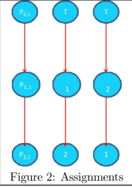
figure below, 0(
01) = 11 and 0(11) = 21. Now there are two assignments A
andB. A() ={1}and A(1) ={2} while B() ={2}and B(2) ={1}.
P0,1
P1,,1
P2,1
T
1
2
T
2
[image:12.595.238.372.245.435.2]1
Figure 2: Assignments
A particularly neat way to avoid this rather cumbersome notation is to simply permute the agents. Let : → be a permutation of players. Then, if is the initial relational mapping in some assignment, this permutation automatically creates a new assignment with a corresponding relational mapping () where
() (()) = {()∈| ∈()}
for each∈. The position of player() = in the new assignment is same as the
position of playerin the initial assignment. For instance, in going fromAtoBin the
figure above, the relevant permutation is(1) = 2 and (2) = 1. Thus, if we fix an
initial assignment, there is bijective relationship between the set of assignments and the set of permutations and any assignment can be represented by a permutation. In what follows, a hierarchy will be denoted by(0 0)and the relational structure in an assignment either by (initial assignment) or by () (the new assignment created
shall extend the notation from individual players to coalitions of players. Namely,
for all ⊆,
() ={()|∈}
Since each assignment is associated with an unique relational structure among players (as opposed to positions), the terms assignment and relational structure will be used interchangeably.
Lemma 2 Consider two assignmentsA andBwith relational structures and()
respectively. Let b ={∈|() =} and bb ={∈|()6=}
(i) If ⊆b, |()|=¯¯()()¯¯
(ii)If bb ⊆, |()|=
¯
¯()()
¯ ¯
Proof. We start with (i). Let 0 ={∈0|
A()∈}. Now, |()| = |0(0)|.
Given that agents in have not changed their positions, {∈0|
B()∈} = 0. Hence, ¯¯()()¯¯=|0(0)| Hence, |()|=
¯
¯()()¯¯
Next, we come to (ii). Again, let 0 = {∈0|
A()∈}. Now, |()| =
|0(0)|. This time while some agents in have changed their positions, the changes
do not involve positions outside 0. Hence, again {∈0|
B()∈} = 0. Thus, ¯
¯()()
¯
¯=|0(0)| Hence, |()|=
¯
¯()()
¯ ¯.
Then, we have the following proposition as a direct consequence of Lemma 2.
Proposition 3 Consider two assignments A and B with relational structures and
() respectively such that () = and () = and() = for each ∈ such that 6= . Then,
(A)− (B) = X
=∪{} ⊆\{}
[∆()−∆(())]
"
1
|()()|−
1
|()| #
Proof. From Lemma 2, for each ⊆ such that ⊇ { }, we have |()| =
changes by:
(A)−(B) = X
⊆ ∆() |()()| − X ⊆ ∆() |()| = X ⊆ ∈ ∈ ∆() |()()| + X ⊆ ∈ ∈ ∆() |()()| −X ⊆ ∈ ∈ ∆() |()|− X ⊆ ∈ ∈ ∆() |()| = X ⊆ ∈ ∈ ∆() " 1 |()()| − 1 |()| # +X ⊆ ∈ ∈ ∆() " 1 |()()| − 1 |()| # = X =∪{} ⊆\{} ∆() " 1 |()()| − 1 |()| # + X =∪{} ⊆\{} ∆() " 1 |()()| − 1 |()| # (5)
Now, for any coalition =∪{}, where ⊆\{ }, replacing by produces () =∪{}. Hence, there is a bijective relation between the set of coalitions given
byΩ={| =∪{} with ⊆\{ }}andΨ={| =∪{} with ⊆\{ }} given by the function :Ω→Ψ. This implies we re-write (5) as follows:
(A)−(B)
= X =∪{} ⊆\{} " ∆() Ã 1 |()()| − 1 |()| ! +∆(()) Ã 1 |()(())| − 1 |(())| !# . (6)
Now, the set of positions occupied by players in the coalition under the relational
structure are occupied by the players in the coalition (), under the relational
structure()and are given by, say,0 ={∈0|
(6) as
(A)−(B)
= X
=∪{} ⊆\{}
"
∆()
Ã
1
|()()| −
1
|()|
!
+∆(())
µ
1
|()| −
1
|(())|
¶# . (7)
Next, we shall show that |()()| = |(())|. = ∪ {} for some =
\ { }. () = ∪{}. First, consider the set of positions occupied by in
the relational structure (). It is given by {∈0|
B()∈∪{}} = 0 (say). Next, consider the set of positions occupied by () in the relational structure . It is given by {∈0|
A()∈∪{}} =0. Since occupies the same position in assignment B as occupies in assignment A, and the positions of players in the set are identical in both assignments, 0 = 0, namely the set of positions occupied by in the relational structure()is the same as the set of positions occupied by
() in the relational structure . Therefore, |()()| = |(())| = |0(0)|.
Hence, we can re-write (7) as
(A)−(B)
= X
=∪{} ⊆\{}
∆()
"Ã
1
|()()| −
1
|()| !
+∆(())
Ã
1
|()| −
1
|()()| !#
= X
=∪{} ⊆\{}
[∆()−∆(())]
"
1
|()()| −
1
|()|
#
(8)
The reader may verify that (8) morphs into (4), when we restrict ourselves to additive games since non-singleton coalitions have a Harsayni dividend of zero.
Now, consider a coalition in (8). Observe that if ({}) ({}), then the
∆()−∆(()) is strictly positive for singleton coalitions and non-negative for
non-singleton coalitions if the game belongs to the class ∗. However, even if the
level occupied by player in assignment A is greater than that occupied by player
, the expression 1
|()()| −
1
Example 4 Consider the following assignment shown in the figure below.
T
5
7
9 2
4
8 6
3
Figure 3: Switching positions
Let (2) = 6, (6) = 2 and () = for 6= 26. For = {28}, () = {68}. Hence,
1
|()()| −
1
|()|
= 1 6−
1 5 =−
1 30
Only for special trees, namely, vertical hierarchies, is the aforesaid expression always non-negative. This is proved in the next lemma. But before that let us introduce the level of a player (as opposed to a position) in an assignment sayA. For all ∈ , define () = () where ∈ 0 is such that A() = and is the relational structure associated with A.
Lemma 3 Consider a vertical hierarchy and an assignment A (with associated rela-tional structure). Let and be such that() (). Consider a permutation
such that () = and () = and () = for each ∈ such that 6= . Then, for all ⊆ such that =∪{} for some ⊆\{ }, we get
1
|()()|−
1
Furthermore, if =∅, then,
1
|()()| −
1
|()| 0
Proof. Let us begin by considering non-empty. Let the highest level among all members of in assignment A be given by. Namely,
= max{()|∈}
Since in a vertical hierarchy, no two players have the same level, 6=()6=().
We can discern three cases: Case 1: () ()
In this case, |()()|=() + 1 and|()|=() + 1. Therefore,
1
|()()|−
1
|()|
= 1
() + 1 −
1
() + 1
= (()−()) (() + 1) (() + 1)
0
Case 2: () ()
In this case, |()()|=+ 1 and|()|=() + 1. Therefore,
1
|()()| −
1
|()|
= 1
+ 1 −
1
() + 1
= (()−) ( + 1) (() + 1)
0
Case 3: () ()
In this case, |()()|=+ 1 and|()|=+ 1. Therefore,
1
|()()| −
1
|()|
= 1
+ 1 −
1
+ 1
= 0
Iffinally, =∅ ={} and
1
|()()|−
1
|()|
= 1
() + 1 −
1
() + 1
= (()−()) (() + 1) (() + 1)
Finally, we can use Lemma 3 and Proposition 3 to arrive at the following result.
Theorem 1 If the TU cooperative game belongs to the class ∗ and the hierarchy is vertical, a complete assignment is optimal if and only if it is cogent.
Proof. Towards a contradiction, consider a complete assignment A (with relational structure) that is optimal but not cogent. Then, there must be at least two agents
and such that() () but() (). Consider an assignment that swaps
these two agents in these positions, namely an assignmentBwith relational structure
() where () = and () = and () = for each ∈ such that 6= .
Then, the payoff of the top agent changes by
(A)− (B) = X
=∪{} ⊆\{}
[∆()−∆(())]
"
1
|()()| −
1
|()| #
(9)
We shall prove that this change (A)− (B)is strictly positive. Consider∆()−
∆(()) where = ∪{} and ⊆\{ }. Now, ∆() − ∆(()) =
∆( ∪{})−∆(∪{}). Given () () and the cooperative game ( )
belongs to the class ∗, it follows that ∆
( ∪{})−∆( ∪{}) > 0. Since the
hierarchy is vertical, by Lemma 3, we get
1
|()()|−
1
|()|
>0
Since the product of two non-negative terms is non-negative, it follows that(A)−
(B) is a sum of non-negative terms and hence is non-negative. To prove that it is positive, we need only prove that one of the terms in the sum of non-negative terms is positive, namely, there exists such that[∆()−∆(())]
h
1
|()()|−
1
|()| i
0. Take ={}. Then, using Lemma 3, we get
[∆()−∆(())]
"
1
|()()| −
1
|()| #
= (({})−({}))
∙
(()−())
(() + 1) (() + 1)
¸
0.
6
Bidding for Positions
6.1
The Two Agent Model
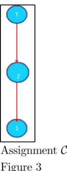
In this section, we shall analyse the situation where two players bid for position in a vertical hierarchy and we arrive at some rather interesting results. Suppose we consider a vertical hierarchy with just two levels and two agents to fill these two
levels. The hierarchy is given in thefigure below.
T
P1,,1
P2,1
Figure 1
Let the productivity of the two agents be given by 1 and 2 where 1 2.
We restrict ourselves for time being to the additive game. The permission value associated with position is given by . Now there are two possible assignments which we refer to asB andC. We depict them below. B is cogent while C is not.
T
1
2
T
2
1
[image:20.595.280.350.68.246.2]Assignment C Figure 3
In assignmentB, the permission values of the three agents are as follows:
(B) = 1 2 +
2
3 ;
1(B) = 1 2 +
2
3 ;
2(B) =
2
3
In assignmentC, the permission values of the three agents are as follows:
(C) = 1 3 +
2
2 ;
1(C) = 1 3 ;
2(C) =
1
3 +
2
2
While the top agent would like a cogent hierarchy, there may be an information asym-metry in the sense that he may not be aware of the productivities of the agents. If he knows which agent is more productive, he can assign them in the designated posi-tions. Hence, for a genuine problem, we shall assume an extreme form of asymmetry namely, he is not aware of which agent is more productive in thefirst place. Assume
that the workers know each other’s productivity. Let us start with the most simple mechanism, namely, workers submits bids and the person with the highest bid gets the higher position. If the bids are identical, then the tie is broken by tossing a coin. Hence, for an assignment A, if is the bid for agent, then payoffof agent is
=(A)−.
Of course, the assignment that will result is a function of the bids. Therefore,
if 1 6=2; where
A(1 2) =
½
B if 1 2;
C if 1 2;
On the other hand, if 1 =2, then,
(1 2) =
1
2(B) + 1
2(C)−.
We shall assume that bids take place in increments of starting from zero. Further-more, all the permission values constitute valid bids. Namely, for any permission value , there exists a positive integer such that = ·. is a sufficiently
small positive real number.
6.2
Best Response Correspondences
We begin by showing that matching a bid is a “never best response” strategy.
Lemma 4 Let the best response correspondence of player be given by(−)given
that the other player bids −. Then,
− ∈ (−).
Proof. Suppose player bids−. Then, his payoffis given by
1
2(B) + 1
2(C)−− (10)
If on the other hand, he bids−+, his payoffis
(B)−−− (11)
if = 1 and
(C)−−− (12)
if = 2.
Start with= 1. 1(B)−1(C) =
1
6 +
2
3 0. Now, (11) is greater than (10) if 1
2[1(B)−1(C)]− 0
or,
1
12+
2
6 .
Assuming is sufficiently small, this will be the case. The proof for = 2is similar.
Lemma 5 For any arbitrary −, (−)⊂{0 −+}.
Proof. We prove the lemma for = 1. The proof for = 2 is similar. Given that
the player is never bid − by Lemma 4, there are two possibilities. Either −
or −. Consider the first case. In this case,
=(B)−.
The payoffis strictly decreasing in and hence, the maximum payoffis obtained by
minimizing subject to the constraint that −. This is precisely−+.
Next, consider the case −. In this case,
=(C)−.
Again the payoff is decreasing in and so is maximized by choosing the minimum
feasible which is zero.
Next, we focus on which of the two bidding strategies will be chosen given a certain bid by the other player. This is shown by the next lemma.
Lemma 6 There exists a certain critical threshold for player such that:
(i) If − , then(−) ={−+}
(ii) If − , then (−) ={0}
(iii) If − =, then(−) ={−+0}
Proof. We prove the lemma for = 1. The proof for= 2 is similar. From Lemma 5, playerwill either bid−+ or, zero. The payoffs are respectively(B)−−−
and(C). Hence,
(B)−−− (C)
⇔ − (B)−(C)−
Similarly,
(B)−−− (C)
⇔ − (B)−(C)−
Finally,
(B)−−− = (C)
⇐⇒ − =(B)−(C)−
Hence, assuming =(B)−(C)−, the lemma is proven.
Now,
1 = 1(B)−1(C)−
= 1 6 +
2
and
2 = 2(C)−2(B)−
= 1 3 +
2
6 −
6.3
The Simultaneous Bidding Game
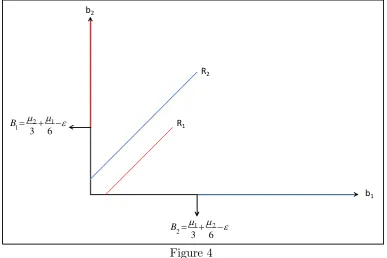
Consider the bidding game where both players bid simultaneously. We begin by showing that this game does not admit a Nash equilibrium.
Lemma 7 The simultaneous bidding game does not admit a Nash equilibrium.
Proof. Towards a contradiction, suppose a Nash equilibrium (∗1 ∗2) exists. Then,
∗2 ∈ 2(∗1) and
∗1 ∈ 1(∗2)
We consider three separate cases.
Case 1: Suppose ∗1 = 0. Then, ∗2 ∈ 2(1∗) = 2(0) = {}. But 1(∗2) =
1() ={2·} and0∈1() which is a contradiction.
Case 2: Next, suppose ∗
2 = 0. We can arrive at a contradiction by a method
similar to Case 1. Case 3: Suppose ∗
1 6= 0 and ∗2 6= 0. By Lemma 5, ∗1 = ∗2 + and∗2 = ∗1 +
simultaneously which is an impossibility.
The diagram below given further insights into the non-existence of a Nash equi-librium. We plot the best response correspondences and find that there is no point
b1 b2
R2
R1
6 3
2 1 2 B
6 3
[image:24.595.122.510.98.356.2]1 2 1 B
Figure 4
6.4
The Sequential Bidding Game
Next, we consider sequential bidding. Suppose 1 bids first followed by 2. First, 1’s
profit function is given by
1(1 2) =
⎧ ⎪ ⎨ ⎪ ⎩
1(B)−1
1
21(B) + 1
21(C)−1
1(C)−1
if 1 2;
if 1 =2;
if 1 2
Now, given that 1 is the first mover, he anticipates 2’s moves from her reaction function, and hence we can replace 2 by elements of 2(1) where 2(1) derived
earlier was given by:
2(1) =
⎧ ⎪ ⎪ ⎪ ⎪ ⎨ ⎪ ⎪ ⎪ ⎪ ⎩
{1+} if 1
1
3 +
2
6 −
{1+0}if 1 =
1
3 +
2
6 −
{0} if 1
1
3 +
2
6 −
Therefore,1’s profit function is given by
b
1(1) = 1(1 2(1)) =
⎧ ⎪ ⎪ ⎪ ⎪ ⎨ ⎪ ⎪ ⎪ ⎪ ⎩
1(B)−1
(1(B)−1) + (1−) (1(C)−1)
1(C)−1
if 1
1
3 +
2
6 −;
if 1 =
1
3 +
2
6 −;
if 1
1
3 +
2
6 −
⇒ b1(1) =
⎧ ⎪ ⎪ ⎪ ⎪ ⎨ ⎪ ⎪ ⎪ ⎪ ⎩ 1 2 + 2
3 −1
³1
2 +
2
3
´
+ (1−)³1 3
´
−1
1
3 −1
if 1
1
3 +
2
6 −;
if 1 =
1
3 +
2
6 −;
if 1
1
3 +
2
6 −
where is some real number such that0661representing an arbitrary
probabil-ity. Treating the three possibilities of (??) as three cases, in each case the payoffs are decreasing in 1. So, we can restrict attention to only those possibilities where the
value of 1 is the minimum feasible number. This gives rise to the following payoff
function.
b
1(1) =
⎧ ⎪ ⎪ ⎪ ⎨ ⎪ ⎪ ⎪ ⎩ 1 2 + 2 3 − 1 3 − 2 6
³1
2 +
2
3
´
+ (1−)³1 3
´
− 1 3 −
2
6 +
1
3
if 1 =
1
3 +
2
6 ;
if 1 =
1
3 +
2
6 −;
if 1 = 0
= ⎧ ⎪ ⎪ ⎪ ⎨ ⎪ ⎪ ⎪ ⎩ 1 6 + 2 6
³1
6 +
2
6
´
−(1−)³2 6
´
+ 1
3
if 1 =
1
3 +
2
6 ;
if 1 =
1
3 +
2
6 −;
if 1 = 0
Two fact emerge from (??). First,1will be averse to bidding1 =
1
3 +
2
6 −because
bidding higher will almost always yield a higher (expected) payoff.2 Second, given 1
6 +
2
6
1
3 , in equilibrium he will bid zero. 2will bid. We summarize this result
in the form of a lemma below.
Lemma 8 In the bidding game where 1 is thefirst mover and 2bids second, there is an unique SPNE in which 1bids zero and 2 bids . The assignment that results is C. The surplus extracted is .
2There is an extreme case where player2 actually chooses = 1 (or sufficiently close to 1) in
which case bidding 1 = 1 3 +
2
6 − actually gives a higher payoff. But that does not alter our
The next case we will handle is sequential bidding where2is thefirst mover. The
reaction function of 1 derived earlier is given by:
1(2) =
⎧ ⎪ ⎪ ⎪ ⎪ ⎨ ⎪ ⎪ ⎪ ⎪ ⎩
{2+} if 2
2
3 +
1
6 −
{2+0}if 2 =
2
3 +
1
6 −
{0} if 2
2
3 +
1
6 −
Therefore,2’s profit function is given by ( is a real number such that 06 61),
b
2(2) = 2(1(2) 2) =
⎧ ⎪ ⎪ ⎪ ⎪ ⎨ ⎪ ⎪ ⎪ ⎪ ⎩
2(C)−2
(2(C)−2) + (1−) (2(B)−2)
2(B)−2
if 2
2
3 +
1
6 −;
if 2 =
2
3 +
1
6 −;
if 2
2
3 +
1
6 −
⇒ b2(2) =
⎧ ⎪ ⎪ ⎪ ⎪ ⎨ ⎪ ⎪ ⎪ ⎪ ⎩ 1 3 + 2
2 −2
³1
3 +
2
2 −2
´
+ (1−)³2 3 −2
´
2
3 −2
if 2
2
3 +
1
6 −;
if 2 =
2
3 +
1
6 −;
if 2
2
3 +
1
6 −
⇒ b2(2) =
⎧ ⎪ ⎪ ⎪ ⎪ ⎨ ⎪ ⎪ ⎪ ⎪ ⎩ 1 3 + 2
2 −2
³1
3 +
2
2
´
+ (1−)³2 3
´
−2
2
3 −2
if 2
2
3 +
1
6 −;
if 2 =
2
3 +
1
6 −;
if 2
2
3 +
1
6 −
Again, since the payoffs are decreasing in2, we restrict ourselves to situations where
2 is the minimum feasible number. Therefore,
b
2(2) =
⎧ ⎪ ⎪ ⎪ ⎨ ⎪ ⎪ ⎪ ⎩ 1 6 + 2 6
³1
3 +
2
2
´
+ (1−)³2 3
´
− 2 3 −
1
6 +
2
3
if 2 =
2
3 +
1
6 ;
if 2 =
2
3 +
1
6 −;
if 2 = 0
= ⎧ ⎪ ⎪ ⎪ ⎨ ⎪ ⎪ ⎪ ⎩ 1 6 + 2 6
³1
6 +
2
6
´
−(1−)³1 6
´
+ 2
3
if 2 =
2
3 +
1
6 ;
if 2 =
2
3 +
1
6 −;
if 2 = 0
Since 1
6 +
2
6
2
3 , the optimal strategy for 2 is to bid 2 =
2
3 +
1
6 .
3 Player 1
bids zero again. We summarize this in form of the following lemma.
3There is a possibility of winning more by bidding less but the risks are quite high and the
Lemma 9 In the bidding game where 2 is the first mover and 1 bids second, there is an unique SPNE in which 1 bids zero and 2 bids 2
3 +
1
6 . The assignment that
results is C. The surplus extracted is 2
3 +
1
6 .
So, we get quite a perverse result in the sense that sequential bidding always results in a non-cogent hierarchy.
Let us now examine when is it optimal to organize such an auction. Without an auction, the top agent’s expected payoff is 5
12(1 +2) given that he does not
know productivities and assigns agents arbitrarily. With an auction, his payoff is µ
22
3 + 51
12
¶
+
2 which includes both the payofffrom the non-cogent hierarchy and
the surplus extracted. So, it is always beneficial to assign agents using an auction, if
the procedure is not too costly to organize because the surplus extracted is greater than the loss of payoffdue to a non-cogent hierarchy.
7
Conclusion
We have therefore shown that where payoffis determined by the permission value in regular hierarchies under additive games, cogent and efficient hierarchies coincide and the result can be extended to non-additive games with appropriate restrictions on the value function. We also study auctioning these positions using a bidding mechanism in simple hierarchies and these always result in a non-cogent hierarchy.
Topics for further research include what auction mechanism can result in a cogent hierarchy and whether the result can be extended to more complicated hierarchies. Also, implications for the size of the firm may be studied. Williamson (1967) study
a model in which control reduces with increasing hierarchical firm depth and this
determines the size of thefirm. Ruys and van den Brink (1999) study a model similar
to others where workers are also paid the permission value in regular hierarchies. However, only the workers in the front positions are productive and all other members of the hierarchy earn positional rents from those workers. The depth of the hierarchy is then determined by the reservation wage. Similar issues can be studied in our model.
References
[1] Brink, R. van den and R.P. Gilles (1996) “Axiomatizations of the Conjuctive Permission Value”, Games and Economic Behavior, 12, 113-126.
[3] Gilles, Robert.P.and Guillermo Owen (1999), “Cooperative Games and Disjunc-tive Permission Structures” Center for Economic Research Discussion Paper 1999-20, Tilburg University.
[4] Gilles, Robert.P., Guillermo. Owen and Rene. van den Brink (1992) “Games with Permission Structures: The Conjunctive Approach”,International Journal of Game Theory, 20 , 277-293.
[5] Lazear, Edward P. and Sherwin Rosen (1981) “Rank-Order Tournaments as Optimum Labor Contracts”, Journal of Political Economy, 89, 841-864.
[6] Myerson, Roger B. (1977) “Graphs and Cooperation in Games”,Mathematics of Operations Research, 9, 169-182.
[7] Rajan, Raghuram G. and Luigi Zingales (2001) “The Firm as a Dedicated Hier-archy”, Quarterly Journal of Economics, 116, 805-851.
[8] Ruys, P.H.M and R. van den Brink “Positional Abilities and Rents on Equilib-rium Wages and Profits” in The Theory of Markets ed. P.J.J. Herrings, G. van
der Laan and A.J.J. Talman, North Holland, 261-269.
[9] Stole, Lars A. and Jeffrey Zweibel (1996); “Organizational Design and Tech-nology Choice under Intrafirm Bargaining”,American Economic Review, 86 , 195-222.
[10] Williamson, Oliver E. (1967) “Hierarchical Control and Optimum Firm Size”,