Was there a "Greenspan conundrum" in the Euro area ?

Munich Personal RePEc Archive

Was there a "Greenspan conundrum" in

the Euro area ?

Lamé, Gildas

INSEE, CREST

September 2013

Online at

https://mpra.ub.uni-muenchen.de/55370/

Was there a ”Greenspan conundrum” in the Euro area ?

∗

Gildas Lam´

e

September 2013

Abstract

This paper implements an affine term structure model that accommodates ”unspanned” macro risks for the Euro area, i.e. distinct from yield-curve risks. I use an averaging-estimator approach to obtain a better estimation of the historical dynamics of the pricing factors, thus pro-viding more accurate estimates of the term premium incorporated into the Eurozone’s sovereign yield curve. I then look for episodes of the monetary cycle where long yields display a puzzling behavior vis-`a-vis the short rate and its expected average path in contrast with the Expectation Hypothesis. The Euro-area bond market appears to have gone through its own ”Greenspan conundrum” between January 1999 and August 2008. The term premium substantially con-tributed to these odd phenomena.

JEL classification: C51; E43; E44; E47; E52; G12

Keywords: Affine term structure models; Unspanned macro risks; Monetary policy; Expec-tation Hypothesis; Term Premium

∗_{A previous version of this paper was circulated under the title: ”The sovereign bond term premium of the Euro area”.}

We thank Jean-Paul Renne for stimulating discussions at the starting phase of this project and for useful comments. We also thank ´Eric Dubois, Christian Gouri´eroux, Nikolay Hristov, Jean-St´ephane M´esonnier, Alain Monfort, Fulvio Pegoraro, Pierre-Alain Pionnier, participants to the INSEE internal seminar, CREST Financial Econometrics seminar, the Third Humboldt-Copenhagen Conference on Financial Econometrics and the 17th International Conference on Macroeconomic Analysis and International Finance for insightful guidance and comments. The views expressed herein are those of the author and do not necessarily reflect those of INSEE. All remaining errors are mine.

†_{INSEE - Macroeconomic Research Division, CREST - Finance and Insurance Laboratory, 15 boulevard Gabriel P´eri}

1

Introduction

In February 2005 during a speech before Congress, former Federal Reserve chairman Alan Greenspan noted that the 10-year treasury yield failed to increase significantly so far despite the 150-basis-point increase in the federal funds rate. This behavior was puzzling with respect to the prevailing term structure theory called the ”Expectation Hypothesis” as long rates should have also increased mechanically. While Greenspan mentioned several possible explanations for the phe-nomenon such as the global savings glut, the origin of this ”conundrum” was left without any precise answer at that moment. In a later monetary policy testimony in July 2005, Greenspan emphasized that yields can be divided into two components: the first one reflecting short-rate expectations and the second one a risk compensation. He suggested the prominent role of this second component in the relatively stable levels of long-term interest rates. Previous studies suggested that this risk premium in the US is time-varying and substantial, thus complicating the transmission of monetary policy as it blurs the relationship between short-term interest rates controlled by central bankers and the long-term ones.

As the sovereign yield curve matters for businesses and households in the Eurozone through the interests paid on long-term savings and putting aside the current problems due to the sovereign debt crisis, one central question naturally follows: in parallel with the American conundrum, were there any periods before the crisis when long rates did not seem to be responsive to changes in the policy rate in the Eurozone? That is, was there also a ”Greenspan conundrum” in the Euro area? If the answer is positive, was the term premium behind this result? These questions are deemed essential if one assumes the Expectation Hypothesis should hold. Under this framework, long yields should be equal to the average expected path of the short rate. Assessing the relative role of the term premium in shaping long-term interest rates can also help policymakers in their evaluation of the transmission channel between the policy rate and long-term yields. Affine term structure models represent one way to answer this question. Naturally, macroeconomic factors ought to play a significant role in the determination of short-rate expectations and risk premia. Therefore, a dynamic term structure model which includes not only the standard ”level”, ”slope” and ”curvature” factors but also macroeconomic factors is welcomed.

relationships among state variables and by minimizing the long-term forecast errors of the state variables, the implemented methodology provides better estimates of long-term expectations of the short rate and thus more accurate long-horizon term premium. Given the unknown nature of the premium’s determinants, my estimate should be viewed as capturing any effects that might impact the price of Euro-area riskless sovereign bonds other than expected future monetary policy. Focusing on the 5Y maturity for the Eurozone, I find that the 5Y yield term premium has been hovering around 100 basis points and represent on average over the period 21% of the 5Y bond yield. All in all, under the framework of the Expectation Hypothesis, the Euro area also went through its own ”Greenspan conundrum”. I distinguish three noteworthy ”conundra” episodes from 1999 to 2008. Similar to past US analyses, two of them took place during monetary policy tightenings decided by the ECB. The third one deserves particular attention as it took place at the same time as the US bond market’s conundrum between June 2004 and December 2005. The estimated affine term structure model uncovers the potential disruptive role of the term premium in the transmission of monetary policy. The various conundra illustrate the difficulties faced by central banks in guiding interest rate expectations towards their desired path as well as in taming the term premium.

2

Related literature

Several papers develop yield curve models without any macroeconomic component such as the popular factor models of Duffie and Kan (1996) or Dai and Singleton (2000), in which the set of yields is explained by a few latent factors. Joslin et al. (2011) among others develop an affine term structure model with only observable factors. And finally, a number of papers model the joint dynamics of the macroeconomy and interest rates such as Ang and Piazzesi (2003). In addition to three latent factors, Ang and Piazzesi (2003) also include two macroeconomic variables extracted from the PCA (Principal Component Analysis) on a set of inflation-related measures and on another set reflecting real activity. But the majority of these macro-finance models make the implicit assumption that macroeconomic variables are actually risk factors that can be derived from yields. On the contrary, Joslin et al. (2013) introduce affine term structure models with observable yields and macro factors that accommodate unspanned macro risks (see section 3.3).

The methodological issues mentioned above are essential to correctly study the conundrum which has been extensively explored by the literature for the US. Many contributions focus on the term premium which estimation has been very challenging. Several papers, such as Bernanke et al. (2004), Cochrane and Piazzesi (2009), Kim and Wright (2005) attempt to obtain a precise estimation of the US term premium. As for the conundrum itself, Kim and Wright (2005) find that a declining term premium was the key factor behind the puzzling behavior of long-term interest rates. In the same vein, Rudebusch et al. (2007) compare several term premium’s estimates and find a similar result.

However, the structural determinants of this risk premium themselves are still not well understood and the search for these fundamental-based macroeconomic factors remains a work in progress. Piazzesi and Schneider (2007) or Bansal and Shaliastovich (2013) for example develop utility-based models for the term structure of interest rates. They both show that inflation underpins the bond risk premium. On the empirical side, the literature highlights a wide range of potential determinants found in the data (the present paper does not attempt to find them). Wright (2011) finds that inflation uncertainty is a significant determinant with a cross-country analysis. Turning again to the conundrum, Kim and Wright (2005) note that practioners often cite several possible factors. Better-anchored inflation expectations with a reduction in macro volatility are one plausible explanation. Analysts also cite the increased foreign interest in US long-term bonds. Moreover, Rudebusch and Swanson (2008) underline the significant role of some ”out-of-model” variables during the conundrum such the volatility of long-term treasury yields, foreign official purchase of Treasury bonds etc. Generally speaking, supply/demand adequation can be said to be the main cause of the conundrum in the US but remain to be fully incorporated in a term structure model.

3

A term structure model with macro factors

3.1

Term premium

Financial theory states that the term structure of interest rates is governed by what is usually called the ”Expectation Hypothesis” (EH). According to this hypothesis, the expected return an investor expects from holding a long-term bond until maturity is the same as the expected return one gets when rolling over a series of short-term bonds. Equivalently, the long-term yield is equal to the average expected short-term yield. Unfortunately, with risk-averse investors, this hypothesis is unlikely to hold, given that a compensation may be required by them in order to hold such bond. The term premium refers exactly to this compensation for bearing the risk of variation in the riskless rate. In this paper, I will only consider the following term premium:

Y ield premium:Y T Ptn=ytn−

1 n

n_X−1

i=0

Et(rt+i) =ytn−Expnt (1)

Herertdenotes the short rate i.e. the one-period yieldy1t,ynt the yield of an-period zero-coupon

bond and Expnt = n1 n_P−1

i=0

Et(rt+i), the expected average path of the short rate over the next n

3.2

The general setup

Following Ang and Piazzesi (2003), I present below the standard discrete-time affine term struc-ture model used as the basis for the paper’s model that incorporates unspanned macro risks as developed in Joslin et al. (2013).

LetPtbe aN1-dimensional vector of pricing factors,MtaN2-dimensional vector of macro factors (N =N1+N2) andZt= [Pt, Mt]. Provided the agents value nominal bonds using a restricted set

of factors that takes into account all risks in the economy, the short rate may be modeled, by the following equation:

rt=ρ0+ρ1Zt (2)

As in standard affine term structure models, I suppose the factorsZtfollow a first-order Gaussian

VAR1 _{under the probability measureP:}

∆Zt=K0PZ+K P

1ZZt−1+ ΣZεPZt (3)

whereεP

Zt =εt∼N(0, IN) and ΣZ is a non-singularN×N matrix.

Under the assumption of complete markets and no arbitrage, there exists a risk-neutral proba-bility measure that is equivalent to the physical measure (see Appendix A for more details). Under the risk-neutral measure, the state vectors follow an alternative law of motion:

∆Zt=K0QZ+K Q

1ZZt−1+ ΣZεQZt (4)

with³K₀Q_Z, K₁Q_Z´both linearly related to¡KP 0Z, K1PZ

¢

by the market prices of risk. (see Appendix A.2 for further details). Under the risk-neutral measure, states of the world in which investor’s marginal utility is high are in fact overweighed compared to the situation in the physical world.

Within a risk-neutral pricing framework, the price of a zero-coupon bond can be written simply as:

pnt =E Q t " exp à − n X i=0 rt+i

!#

(5)

Plugging Equation (2) into Equation (5), bond prices can be expressed as exponential affine functions of the state variables:

pnt = exp ³

An+B

′

nZt ´

(6)

where the coefficients An is a scalar and Bn is a N ×1 vector for a given maturity. The

continuously-compounded bond yield yn

t is therefore:

1

ytn=An+Bn′Zt (7)

withAn=−An/n andBn=−Bn/n.

3.3

A model with unspanned macro risks

Given Equation (7), both the pricing factorsPtand the macro factorsMtdetermine the

model-implied bond yields. With the bond yields as given, one would be able to solve for the factors using (7) and would conclude thatMt is ”spanned” by bond yields, i.e. perfectly replicated such as

Mt=a0+a′1Pt (8)

However, empirical results (see Ludvigson and Ng (2009) for example) show that macro factors (such as economic growth and inflation) are only partially explained by Pt, which is actually in

line with the general conception that risks ranging from financial to labor markets, and not only sovereign bond yields, impact real economic growth.

Equation (8) also implies that after conditioning on the current yield curve, the macro variables Mt are supposed to have no additional information content on risk premiums and future values of

Mt. Again, as Joslin et al. (2013) already emphasize, this feature is in contradiction with the vast

literature on business cycle forecasting.

Furthermore, as the cross section of bond yields is actually well explained by a very small number of factors (typically the level, slope and curvature for most developed bond markets), the standard term structure model presented above, with its additional spanned macro factors, is also plagued by a poor goodness-of-fit as noted by Joslin et al. (2013).

The several issues associated with the spanned macro factors of the standard model hint that the initial framework is somehow flawed. Joslin et al. (2013) suggest that what has to be reconsidered is the hypothesis that the discount factor agents use to price bonds is fully responsive to macro risks. If we assume now that agents’ pricing kernel results from the projection of the economy-wide kernel (based onZt) on the limited set of factors that explains the term structure of the yield curve (only

Pt) instead, then the issues raised above become irrelevant. Under this modified framework, the new

SDF prices the entire yield curve but not all macro risks which are now ”unspanned” by information on the yield curve, i.e. imperfectly correlated.

As developed in Joslin et al. (2013)2_{, the new assumption entails that Equation (2) and (4)}3 become

rt=ρ0+ρ1PPt (9)

∆Pt=K₀Q_P+K₁Q_PPt−1+ ΣPεQ_Pt (10)

2

Like these authors, I also suppose that the inclusion of spanned or unspanned macro factors in the affine term structure model is independent of the issue of bond yields’ or macro factors’ measurement errors.

3

with ρ1P and K₀Q_P two N1-dimensional vectors, K₁Q_P a N1×N1 matrix, ΣPΣ′P the N1×N1 upper-left block of ΣZΣ′Z andε

Q

Pt ∼N(0, IN1).

It can be shown that under the new framework, the lastN2elements ofBnare equal to 0. Thus,

Equation (7) is equivalent to

ynt =Afn+Bfn

′

Pt (11)

whereAfn andBfn are deduced from recursive equations (see Appendix A.2).

In general, affine term structure models provide a simple and flexible framework to study the term structure of interest rates but as the literature previously underlined (see Gurkaynak and Wright (2012)), these simple representations are not based on any structural foundations. Moreover, by introducing unspanned macro factors in the model, I actually assume that the pricing kernel of economic agents does not fully price macro risks. Overall, though having shortcomings, I believe that the model with unspanned macro factors presented here provides a flexible, simple, and parsimonious way to study the term structure of risk-free interest rates in the Eurozone while taking into account important economic features of the term premium in the Eurozone’s bond market.

4

The data

4.1

Yield data

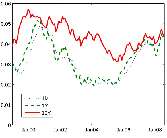
I use data on monthly zero-coupon bond yields of maturities 6, 12, 24, 36, 60, 84 and 120 months from January 1999 to August 2008. The short-term rate used throughout the paper is the 1-month OIS rate rather than the 1-month Euribor in which non-negligible liquidity and credit risk premia are priced. Until September 2004, I use the German sovereign yield curve (provided by the Bundesbank) as representative of the Euro area risk-free interest rates. From October 2004 to August 2008, zero-coupon bond yields provided by the ECB for the Eurozone AAA countries are used in this paper. All yield data are end-of-month. Some of the sovereign yields are plotted in Figure 1.

According to Joslin et al. (2011),Ptcan be rotated to become the principal components of bond

yields. A PCA shows that the first three principal components of bond yields explain 99.9% of the cross-sectional variation. I choose to use the first N1 = 3 P Cs of bond yields4 , that are usually interpreted as the level, slope and curvature of the yield curve as the yield pricing factorsPt.

Table 1 reports some descriptive statistics of the various bond yields used in the sample.

4

Like others in the literature (Joslin et al. (2013) for example), I rescale the principal components obtained from the PCA. we denotelj,i the loading on yieldiin the construction ofP Cj, theP Cs have been rescaled so that: (1)

P8

i=1l1,i/8 = 1, (2)l2,10Y−l2,6M = 1 and (3)l3,10Y−2l3,2Y+l3,6M = 1. This way, theP Cs are on a similar scale.

Jan00 Jan02 Jan04 Jan06 Jan08 0

0.01 0.02 0.03 0.04 0.05 0.06

1M 1Y 10Y

Figure 1: Eurozone historical zero-coupon bond yields for three different maturities.

Jan00 Jan02 Jan04 Jan06 Jan08

0 0.01 0.02 0.03 0.04 0.05 0.06 0.07

PC

1

PC

2

PC

3

Figure 2: Historical series of the first three principal components of bond yields from 1999 to Aug 2008.

4.2

Macro variables

Yields 1M 6M 1Y 2Y 3Y 5Y 7Y 10Y

Mean 0.032 0.032 0.033 0.035 0.036 0.039 0.042 0.044 SD 0.009 0.009 0.009 0.008 0.008 0.007 0.007 0.006 Skewness 0.264 0.253 0.183 0.132 0.143 0.177 0.137 -0.001 Kurtosis 1.844 1.964 1.935 1.955 2.007 2.114 2.181 2.180 Min 0.020 0.019 0.019 0.020 0.022 0.025 0.028 0.031 Max 0.049 0.051 0.052 0.053 0.053 0.053 0.055 0.057

Table 1: Summary statistics on Euro Area monthly zero-coupon bond yields. Period: 1999M1-2008M8

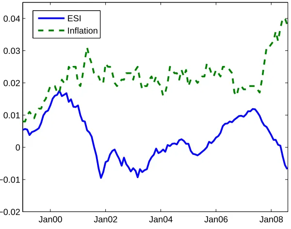
real activity. The second one is the Euro-area monthly year-on-year inflation (HICP, overall index).7 Figure 3 plots the two variables.

Jan00 Jan02 Jan04 Jan06 Jan08

−0.02 −0.01 0 0.01 0.02 0.03

0.04 ESI

Inflation

Figure 3: Time series of Euro-area inflation and of the Economic Sentiment Indicator from 1999 to Aug 2008.

To assess the need for a model that accommodates ”unspanned” macro risks, we can check how well the macro factors are explained by the P Cs. With the present data sample, the projection

contribute to the indicator. The raw indicator is rescaled so that the variable take on values in [−2%,4%]

6

Other activity-related indicators can be used such as the Eurozone industrial output or even an estimated monthly real GDP growth.

7

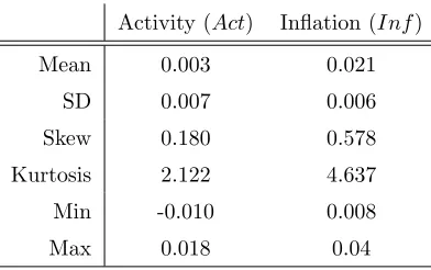
Activity (Act) Inflation (Inf)

Mean 0.003 0.021

SD 0.007 0.006

Skew 0.180 0.578

Kurtosis 2.122 4.637 Min -0.010 0.008

Max 0.018 0.04

Table 2: Summary statistics on Euro area macroeconomic factors. Period: 1999M1-2008M8

of real activity on the first three P Cs of yields gives an adjusted R2 _{of 55% and the projection of} inflation 15%. Thus almost 45% of the variation in activity and 85% of inflation are not related to the yields’P Cs.

Projections of changes in activity and inflation onto changes in the threeP Cs give even smaller adjusted R2 _{(21% and 1% respectively). All in all, accommodating unspanned macro risks in the} Gaussian term structure model is welcomed.

5

Estimation

5.1

First approach

The methodology used for the estimation of the model closely follows Joslin et al. (2013) but without the reparametrization detailed in Joslin et al. (2011), which reduces the number of parame-ters to be estimated and allows for faster computation. Nevertheless, I choose to stick to a standard procedure which will be detailed below to keep the model simple. The parameters to be estimated are included in the following equations under the risk-neutral measure:

rt=ρ0P+ρ1PPt (12)

∆Pt=K0QP+K Q

1PPt−1+ ΣPεQPt (13)

And under the physical measure:

∆Zt=K0PZ+K1PZZt−1+ ΣZεPZt (14)

In the model, theZtare priced without errors (Zt=Zt,o) whereas the zero-coupon bond yields

constraints imposed by the no-arbitrage condition. The conditional likelihood function (underP) of the observed data ¡yn

t,o ¢

can be written as:

f¡ynt,o|ytn−1,o, Zt−1; Θ

¢

=f(ynt,o|Zt;ρ0P, ρ1P, K0QP, K Q

1P,ΣP)∗f(Zt|Zt−1;K0PZ, K1PZ,ΣZ) (15)

As mentioned earlier, I suppose the yields on zero-coupon bondsyn

t,o equal their model-implied

values yn

t,m =Afn+Bfn

′

Pt plus mean zero, i.i.d. and normally distributed errors ηt =yt,on −ynt,m,

which entails:

f(ynt,o|Zt;ρ0P, ρ1P, K0QP, K Q

1P,ΣP) = (2π)−(J−N)/2|Ση|

−1 ×exp µ −1 2 ° °Σ−1

η ×(ηt) ° °2¶

(16)

Using the assumption thatZtis conditionally Gaussian, the second term can be expressed as:

f(Zt|Zt−1;K0PZ, K1PZ,ΣZ) = (2π)−N/2|ΣZ|

−1 ×exp µ −1 2 ° °Σ−1

Z ×(Zt−Et−1[Zt]) ° °2¶

(17)

where Et−1[Zt] = K0PZ + ¡

I+KP 1Z

¢

Zt−1, J is the total number of yield maturities and where for a vector x,kxk2denotes the Euclidean norm squared Px2

i.

The (conditional ont= 0) log-likelihood function is therefore the sum:

L=

T X

t=1

h

loghf(yt,on |Zt;ρ0P, ρ1P, K0QP, K Q 1P,ΣP)

i

+ log£f(Zt|Zt−1;K0PZ, K1PZ,ΣZ) ¤i

(18)

Parameters in Equation (3) can be estimated from time series without considering cross-sectional restrictions : ifZtis priced perfectly by the model (Zt,o=Zt), Joslin et al. (2013) prove that the ML

estimates of ¡KP 0Z, K1PZ

¢

are actually given by the OLS estimation of the V AR(1) process Zt8 and

are independent of (ΣP,ΣZ). The remaining parameters of the model (ρ0P, ρ1P, K0QP, K Q

1P,ΣZ) are

then estimated by maximum log-likelihood, assuming the observed bond yields are measured with an i.i.d Gaussian error.9 _{I choose here not to take into account the internal-consistency constraint} which requires model-implied yields to reproduce theP Cs. Nevertheless, I check that the constraint actually holdsex-post.10

5.2

Near-cointegrated VAR (NCVAR)

Interest rates are well-known to be highly persistent and given the short range of data at my disposal on the Eurozone yield curve, bias can easily arise in the estimation of the historical dynamics of interest rates. Because of high persistence in the data, I face what the literature usually calls

8

Actually, though additional lags should be considered in light of standard lag selection procedures, our sample is too limited in size. Nevertheless, if I consider a VAR(2) process forZt, the estimation shows most coefficients ofZt−2

are not significantly different from 0. Thus, my VAR(1)-based model is still preferable.

9

See Appendix C.2

10

the ”discontinuity problem”, which is the huge difference between predictions (especially long-run forecasts of persistent variables) based on unconstrained VAR models and those taking into account unit-roots and cointegration relationships.

The approach I use to solve these issues is largely drawn from Jardet et al. (2013) and introduces ”Near-Cointegrated VARs” (NCVAR) to get better estimations of long-run expectations, using av-eraging estimators. I call ”CVAR” the model under the historical measure estimated under a VECM framework.

5.2.1 Unit roots and VECM model

Standard unit-root tests reveal that the firstP C, which is a proxy for the level of the yield curve, is closer to a I(1) process or at least very persistent, as well as P C2 and Inf. Results are more mixed for P C3 and the activity factor but given KPSS and ERS’s superior power to the ADF test, P C3 andActare closer to stationarity. In the end, choosing a simple VAR to model the historical dynamics of Zt will most likely lead to significant estimation bias, given the high persistence and

potential cointegration relationships among the five state variables.

The historical dynamics of the factors which is described through Equation (3) can be directly interpreted as a vector error correction model (VECM). I determine the rankrof matrixKP

1Z with

a Johansen cointegration test using a trace and maximum eigenvalue tests. ractually represents the number of cointegrating relationships among the state variables.

By choosing to write the VECM with Equation (3), I actually make the implicit hypothesis that there’s a linear trend inZtor/and an intercept in the cointegrating component11. Equation (3) can

be rewritten as:

∆Zt=α(β′Zt−1+c0) + ΣZεPZt (19)

or

∆Zt=α(β′Zt−1+c0) +c1+ ΣZεPZt (20)

with the decomposition KP

0Z = αc0 ( K0PZ = αc0+c1 respectively). 12 Under the restricted specification (19), the trace and eigenvalue tests both point to the same rank of cointegration. Both tests accept the presence of r= 2 cointegrating relations. Therefore, I can write KP

1Z =αβ

′ _where

11

Critical values of the Johansen test actually depend on the assumptions made concerning the cointegrating relations and the VECM which are:

• absence or presence of an intercept/trend in the cointegrating relations

• absence or presence of an intercept in the VECM (which is equivalent to a linear trend in the data. I choose to neglect quadratic trends).

12

Actually, though additional lags should be considered in light of standard lag selection procedures, our sample is too limited in size. Nevertheless, if I consider a VECM forZtthat also includes ∆Zt−2, the estimation shows most

αis a (5×2) adjustment coefficient vector and β a (5×2) cointegrating vector. The cointegration analysis was based on the model with a restricted constant so I still have to test the hypothesis H0 : K0PZ =αc0 against its alternative Ha : K0PZ = αc0+c1 using a χ2(3)-distributed likelihood ratio statistic (see Johansen (1995)) to confirm that specification (19) is the most appropriate one. The test confirms specification (19) and therefore tells us that there’s no drift in the common trend.13

5.2.2 Averaging estimators

Averaging estimators were first proposed by Hansen (2010). The idea consists in combining two different kinds of estimators. Firstly, I estimate the parameter θU N C of the unconstrained

VAR with one lag representing the historical dynamics of the factors by OLS. In a second step, I proceed with the estimation of a one-lag VECM of the state variables (therefore imposing unit-root constraints), which gives the parameter vector θCON. The averaging estimator that specifies the

Near-cointegrated VAR is then defined as:

θN CV AR=θN CV AR(λ) =λθU N C+ (1−λ)θCON (21)

withλ∈[0,1] a parameter used to minimize a chosen criterion.

Given that the short rate will depend on the yields’ P Cs as stated in Equation (9), I choose to focus on minimizing the forecast error (RMSFE) when predicting the P Cs. As the objective is to provide a more precise estimation of the term premium, I could have actually minimized the error in forecasting the short-rate orExpn

t, given the definition ofY T Ptn in the paper. Jardet et al.

(2013) base their criterion onEQ_t [exp (−(rt+...+rt+h−1))], thus having at disposal more points for the computation of the criterion. Both alternative approaches would have been more relevant but computationally more intensive in the present framework asλ,ρ0, ρ1and the parameters governing the historical/neutral dynamics of the state variables would have to be estimated simultaneously. So the present approach can benefit from the two-step estimation speed.

So for a forecast horizonh, the parameterλ(h) is selected through the following minimization program:

λ∗

(h) = arg min

λ∈[0,1]

X i " X t ³

Pi,t+h−Eimpliedt [Pi,t+h] ´2#

(22)

where Pi,t+h is the observed realization of the P Ci for each date t and horizon h whereas

Eimplied_t [Pi,t+h] is the model-implied prediction of the P Ci. The criterion is just (up to a factor)

the standard T M SF E(Trace Mean Square Forecast Error).

Like for a conventional out-of-sample forecasting exercise, I first estimateθU N C andθCON over

the period 1999M1-2002M0814 _{and compute Pb}

t+h with t = 2002M08. For each later date t, I

re-13

The likelihood ratio statistic isLR=−TP5

j=3log

h³

1−eλj

´

/(1−λj)

i

where³λj,eλj

´

are the smallest eigen-values associated to the maximum likelihood estimation of the unrestricted and restricted model respectively. I find

LR= 0.830 which is much lower thanχ2

0.01(3)=11.35 14

estimateθU N C andθCON over the expanded window and compute the model-implied forecast value

of theP Cs. This methodology replicates the typical behavior of an investor that incorporates new information over time. The out-of-sample forecasts are performed fort∈[2002M09,2008M08−h]. In the end, as I am interested in long-term risk premium, h is set equal to 60 months given the limited time length of the data and the optimization yields λ = 0.3042 with the Trace Root Mean Square Forecast Error (TRMSFE) being equal to 82 bps15_{, while for the VAR-based model} T RM SF EV AR= 109 bps andT RM SF ECV AR= 158 bps for the CVAR-based one. This estimated

value for λimplies thatθN CV AR is something closer toθCON than the VAR-based estimator.

6

Results

6.1

Parameters estimates

ρ0, ρ1P, K0QP, K Q

1P, K0PZ, K Q 1Z,ΣZ

´

16_{are initiated at the values obtained from the estimations of} the associated standard VARs. Maximization of the log-likelihood and computation of the asymp-totic standard errors (for the short-rate and risk-neutral parameters) are performed using the quasi-Newton algorithm available in the Matlab software. Estimates for ³ρ0, ρ1P, K₀Q_P, K₁Q_P

´

are highly significant because the estimation takes advantage of the large cross-sectional information on yields. In the end, the root mean square fitting error of yields is extremely low (around 1 bp), indicating that the first three P Cs are able to account for almost all cross-sectional variation in yields thus proving that the specification of theQ-dynamics of bond yields reflected in Equation (4) and (11) is appropriate for Eurozone data. Observed and model-implied yields almost coincide. For instance, the difference between the observed and model-implied 5Y bond yield never exceeds 7 bps.

6.2

Estimation of the term premium

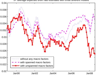
I attempt now to provide an estimate of the Eurozone term premium for the 5Y horizon as the averaging estimator was optimally chosen for this maturity.17 First of all, Figure 4 shows the difference obtained for the model-implied 5-year average expected path of the short rate Exp5Y

t =

1 60

60_P−1

i=0

Et(rt+i) between a simple model without any macro factors, with spanned macro factors and

our baseline NCVAR-based that includes unspanned macro risks. As it is shown in the figure, the unspanned estimate significantly deviates from the other two, especially in 2007-2008. The first two models fail to capture the important fall at the end of the sample. Figure 5 compares instead the different versions based on the VAR-, CVAR- (VECM) and NCVAR-based models with unspanned macro factors. As mentioned earlier, using a simple VAR-based term structure model would lead to

at least consider 5-year-ahead expectations of theP Cs for the estimation strategy.

15

The estimate ofλstays robust after slight changes to the initial time window (see Appendix for details).

16

Tables in Appendix C.4 give the estimated parameters of the term structure model based on the previously described NCVAR method

17

a rather flat 5Y average expected short rate path while the one based on the CVAR model is much more volatile.

Jan00 Jan02 Jan04 Jan06 Jan08

0.02 0.022 0.024 0.026 0.028 0.03 0.032 0.034 0.036 0.038 0.04

5Y average expected short rate estimates with three different models

without any macro factors with spanned macro factors with unspanned macro factors

Figure 4: 5-year average expected path of the short rate extracted from a model without macro factors (blue dotted line), with spanned macro factors (magenta dashed line) and from the baseline NCVAR-based model with unspanned macro factors (red solid line with cross markers)

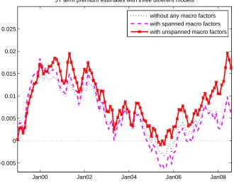
Turning to the term premium, Figure 6 once again reveals the discrepancy between the no-macro/spanned term structure models and our baseline that includes unspanned macro factors. The no-macro and spanned estimate dive clearly into negative territory at the end of the American ”Greenspan Conundrum”. The significant deviation in 2007-2008 is also particularly striking as the baseline estimate strongly rises until August 2008. Obviously, omitting macro factors or enforcing the macro-spanning constraint lead to inaccurate model-implied term premia. Indeed, in both cases, after conditioning on the current yield curve, macro variables are assumed to be uninformative about risk premium. Finally, Figure 7 shows instead the 5Y term premium obtained with the model based on a VAR, CVAR and NCVAR processes. The figure typically illustrates once again the differences between the three methodologies with the VAR-based premium being much more volatile than the others for instance.

Jan00 Jan02 Jan04 Jan06 Jan08 0.02

0.025 0.03 0.035 0.04 0.045

5Y average expected short rate

VAR−based CVAR−based NCVAR−based

Figure 5: Expected average path of the short rate over a 5-year horizon estimated with the VAR-based (blue dashed line), the NCVAR-VAR-based (red dash-dotted line) and the CVAR-VAR-based models (green dotted-line).

7

Was there a bond yield conundrum in the Euro area ?

7.1

A first look

Under the assumption of the Expectation Hypothesis, long rates should be responsive to any change in the short rate and its expected average path. What triggered the debate around the Greenspan conundrum was the muted response of long rates after the successive rate hikes decided by the FED between 2004 and 2006. Thus, in this parallel analysis, I check whether or not the Euro area also experienced the same pattern during its monetary tightening episodes. Figure 8 shows how the 5Y rate evolved throughout the sample’s period compared with its two components (Exp5Y

t and

Y T P5Y

t ) andrtas estimated with the NCVAR model. At first sight, at the start of the first episode

of tightening, from November 1999 to March 2000, the short-term interest rate rose while the 5Y interest rate increased somewhat to around 5.20% with a stagnantExp5Y

t and a volatileY T Pt5Y in

the background.

Jan00 Jan02 Jan04 Jan06 Jan08 −0.005

0 0.005 0.01 0.015 0.02 0.025

5Y term premium estimates with three different models

without any macro factors with spanned macro factors with unspanned macro factors

Figure 6: 5-year term premium extracted from a model without macro factors (blue dotted line), with spanned macro factors (magenta dashed line) and from the baseline NCVAR-based model with unspanned macro factors (red solid line with cross markers)

Apart from these periods discussed above from which a parallel has been drawn with past analyses on the US bond market, Figure 8 reveals an intriguing event. From June 2004 to December 2005, while the US bond market was experiencing its ”Greenspan conundrum”, the Euro area was also going through its own ”euro-conundrum” simultaneously. The short rate was stable during that period but the 5Y bond yield fell dramatically from 3.70% to 2.94%. Turning to the sub-components, the term premium was apparently the major contributor to this significant fall.

Under the framework of the EH and mirroring past US analyses, we see that the Euro area expe-rienced at least three noteworthy phases of puzzling behaviors which we can dub ”euro-conundra”: two of them displaying odd responses from bond yields after rate hikes in a similar fashion to the US experience and a third one which took place simultaneously with the Greenspan conundrum. In all these episodes, the model’s term premium apparently played a significant role, which I will properly disentangle below.

7.2

Contribution analysis

Figure 9 plots the contributions of both the expectation (Exp5Y

t ) and the term premium

com-ponent (Y T Pn

Jan00 Jan02 Jan04 Jan06 Jan08 −0.005

0 0.005 0.01 0.015 0.02 0.025

5Y Term Premium

VAR−based CVAR−based NCVAR−based

Figure 7: 5-year yield term premium estimated with the VAR-based (blue dashed line), the NCVAR-based (red dash-dotted line) and the CVAR-NCVAR-based models (green dotted-line).

confirms the dominant contribution of the 5Y term premium at first to the puzzling behavior of the associated bond yield which did not actually follow the average expected path of the short rate. Similar to what was found by the literature in the US, these movements of the 5Y yield we witnessed at the beginning of the monetary tightening was primarily driven by the term premium according to the model. As our estimate of the term premium is supposed to capture any effect that can impact sovereign bonds’ prices, it is difficult to attribute one precise reason for this significant contribution of the risk premium. At least, given the stability of the average expected path of the short rate, the expected monetary policy effect must have been entirely captured by the term premium instead.

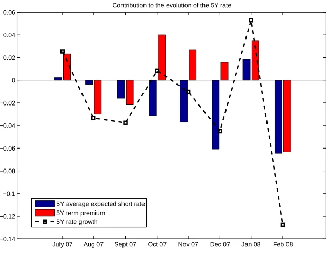
Turning to the second tightening episode in Euro-area history, Figure 10 plots again the contribu-tions of both components associated to the 5Y bond yield. As suspected earlier, the fall of the long rate is actually due to investors’ long-term expectations of the path of rt. This tightening actually

stands out as the financial crisis began to slowly spread to the Eurozone. Investors believed the ECB could not hold for long their strong tightening monetary stance. Thus, it seems they changed their long-term expectations of the short rate’s path in the future and already expected for a more accommodative policy from the ECB.

Jan00 Jan02 Jan04 Jan06 Jan08 0

0.01 0.02 0.03 0.04 0.05 0.06

Figure 8: Evolution of the model-implied short rate (solid line), y5Y

t (model-implied, dotted line),

Exp5Y

t (model-implied, solid line with hollow circle markers) andY T Pt5Y (model-implied, solid line

with full circle markers) over the Eurozone’s previous monetary tightening episodes (shaded in grey).

difficult to uncover the true factors that caused this conundrum at the same time as the American one.

As in the previous sections, I check the results obtained with a no-macro term structure model.18 In contrast to the baseline results above, the contribution of the term premium in 1999 is clearly underestimated in a model without macro factors. The same goes for the average expected path in 2007-2008. Therefore, this discrepancy illustrates again the necessary inclusion of unspanned macro factors. Even though the NCVAR-based model (averaging estimator with unspanned macro factors) is preferable, I also check the results obtained with the VAR-based and CVAR-based con-tributions of the average expected path of the short rate and of the term premium.19 _{The overall} qualitative results are similar though, as expected, slight differences exist because of the nature of the underlying models. For instance, the average expected path of the short rate (Exp5Y

t ) displays

a somewhat more significant contribution under the CVAR-based model, which is mainly due to its higher volatility as we saw with Figure 5 while its contribution is clearly weaker under the VAR setting, thus exaggerating the role of the term premium. All in all, these additional results confirm

18

Figures are provided in Appendix D

19

Nov 99 Dec 99 Jan 00 Feb 00 March 00 −0.06

−0.04 −0.02 0 0.02 0.04 0.06

Contribution to the evolution of the 5Y rate

5Y average expected short rate 5Y term premium

5Y rate growth

Figure 9: Contribution ofExp5Y

t (in blue, left bar) and ofY T Pt5Y (in red, right bar) to the evolution

of the 5-year bond yield (black dashed line) from November 1999 to March 2000.

the relevance of the averaging-estimator-based term structure model when studying the ”Greenspan conundrum”.

From the perspective of monetary policy, under the standard EH framework, the only way for the central bank to control long-term yields is by influencing market expectations of future monetary policy. The results presented here show that long bond yields do not always mechanically follow the short rate and its expected average path. However, under the extended framework of the EH, I find that long-term risk-free yields in the Euro area are buffered by a substantial and time-varying term premium. Thus the central bank not only has to guide market expectations of its future policy but it also has to take measures to alter this risk premium. The selected conundra highlighted here illustrate the difficulties faced by central banks in guiding market expectations as well as in influencing the term premium. On that point, problems in the adequation between the supply and demand of sovereign bonds (due to several structural factors as mentioned in Kim and Wright (2005)) likely drove the term premium downward in the European bond market.

8

Conclusion

July 07 Aug 07 Sept 07 Oct 07 Nov 07 Dec 07 Jan 08 Feb 08 −0.14

−0.12 −0.1 −0.08 −0.06 −0.04 −0.02 0 0.02 0.04 0.06

Contribution to the evolution of the 5Y rate

5Y average expected short rate 5Y term premium

5Y rate growth

Figure 10: Contribution of Exp5Y

t (in blue, left bar) and of Y T Pt5Y (in red, right bar) to the

evolution of the 5-year bond yield (black dashed line) from June 2007 to January 2008.

short rate expectations in determining long-term interest rates. But deviations from the hypothesis primarily stem from investors’ risk aversion, who therefore demand a risk premium.

In this paper, I estimate an arbitrage-free Gaussian term structure model for the Euro area which allows for macro risks to be priced distinctly from the yield curve. Indeed, the state factors of the model include macroeconomic variables which are not entirely spanned by bond yields. I also adopt a relevant estimation approach which yields better term premium estimates than a conventional unconstrained VAR model by using averaging estimators. The estimated term structure is consistent with the Euro area, as unspanned macro risks are taken into account in line with the observed data. Moreover, the econometric methodology used provides more accurate estimates of long-horizon term premium.

June 04 Oct 04 Jan 05 April 05 July 05 Nov 05 −0.08

−0.06 −0.04 −0.02 0 0.02 0.04 0.06 0.08 0.1

Contribution to the evolution of the 5Y rate

5Y average expected short rate 5Y term premium

5Y rate growth

Figure 11: Contribution of Exp5Y

t (in blue, left bar) and of Y T Pt5Y (in red, right bar) to the

evolution of the 5-year bond yield (black dashed line) from June 2004 to December 2005.

References

Ang, A. and Piazzesi, M. (2003), A no-arbitrage vector autoregression of term structure dynamics with macroeconomic and latent variables, Journal of Monetary economics 50(4), 745–787.

Bansal, R. and Shaliastovich, I. (2013), A long-run risks explanation of predictability puzzles in bond and currency markets, Review of Financial Studies 26(1), 1–33.

Bernanke, B., Reinhart, V., and Sack, B. (2004), Monetary policy alternatives at the zero bound: An empirical assessment, Brookings papers on economic activity 2004(2), 1–100.

Cochrane, J. and Piazzesi, M. (2009), Decomposing the yield curve, InAFA 2010 Atlanta Meetings Paper.

Dai, Q. and Singleton, K. J. (2000), Specification analysis of affine term structure models, The Journal of Finance 55(5), 1943–1978.

Duffie, D. and Kan, R. (1996), A yield-factor model of interest rates, Mathematical finance 6(4), 379–406.

Hansen, B. E. (2010), Averaging estimators for autoregressions with a near unit root, Journal of Econometrics 158(1), 142–155.

Jardet, C., Monfort, A., and Pegoraro, F. (2013), No-arbitrage near-cointegrated VAR(p) term structure models, term premia and GDP growth, Journal of Banking and Finance 37(2), 389 – 402.

Johansen, S. (1995), Likelihood-based inference in cointegrated vector autoregressive models. Cam-bridge University Press.

Joslin, S., Priebsch, M., and Singleton, K. (2013), Risk premiums in dynamic term structure models with unspanned macro risks, Journal of Finance, forthcoming.

Joslin, S., Singleton, K. J., and Zhu, H. (2011), A new perspective on gaussian dynamic term structure models, Review of Financial Studies 24(3), 926–970.

Kim, D. H. and Orphanides, A. (2012), Term structure estimation with survey data on interest rate forecasts, Journal of Financial and Quantitative Analysis 47(01), 241–272.

Kim, D. H. and Wright, J. H. (2005), An arbitrage-free three-factor term structure model and the recent behavior of long-term yields and distant-horizon forward rates, FEDS Working Papers (2005-33).

Ludvigson, S. C. and Ng, S. (2009), Macro factors in bond risk premia, Review of Financial Studies 22(12), 5027–5067.

MacKinnon, J. G., Haug, A. A., and Michelis, L. (1999), Numerical distribution functions of likelihood ratio tests for cointegration, Journal of Applied Econometrics 14(5), 563–577.

Piazzesi, M. and Schneider, M. (2007), Equilibrium yield curves, InNBER Macroeconomics Annual 2006, Volume 21, pp. 389–472. MIT Press.

Rudebusch, G., Sack, B., and Swanson, E. (2007), Macroeconomic implications of changes in the term premium, Federal Reserve Bank of St. Louis Review 89(4), 241–269.

Rudebusch, G. D. and Swanson, E. T. (2008), Examining the bond premium puzzle with a DSGE model, Journal of Monetary Economics 55, S111–S126.

A

Appendix: Modeling the yield curve

A.1

Brief reminder

The yield curve is the center of interest for macroeconomists, financial economists and practioners alike.

On the one hand, in the case of macroeconomists, the goal was mostly to assess the impact of various shocks on the yield curve. A first natural approach is the one chosen by ? or Evans and Marshall (1998, 2007) which mainly consists in a unrestricted VAR estimated for a set of yields. Indeed, they include both macroeconomic variables and bond yields of various maturities in a standard VAR process in order to see for instance how exogenous impulses to monetary policy affect bond yields of various maturities. One central drawback of these simple macro models lies in the relatively large number of coefficients to be estimated if we want to consider a broad range of yield maturities. Results might also depend on the set of yields chosen. However, their most critical weakness is that they can allow arbitrage opportunities, i.e. investors can devise a riskless and profitable strategy which consists in buying a long-term zero-coupon bond and selling some combinations of the others in the model.

On the other hand, in the empirical finance literature, macroeconomic linkages are simply ignored and the entire set of bond yields is explained by a few latent factors while taking into account the no-arbitrage restriction. Models developed by Duffie and Kan (1996) and Dai and Singleton (2000) are representative of this class and provide an excellent fit. The factors underlying bond yields have actually no direct economic meaning and do not provide any clue on the macroeconomic forces behind the movements of the yield curve. However, the no-arbitrage restriction enforces the consistency of evolution of the yield curve over time with the absence of arbitrage opportunities. The main drawback of arbitrage-based term structure models is that they have little to say about the dynamics of interest rates as their primary concern is to fit the curve at one point in time and cannot be used for forecasting.

A seminal paper by Ang and Piazzesi (2003) was the first to bridge the gap between these two worlds. They introduce a no-arbitrage term structure model based on the assumption that the short rate depends on some yield-related latent factors and two macroeconomic variables (inflation and a real activity indicator) as with a simple Taylor rule. Their model became the backbone of many macro-finance affine term structure models.

A.2

The framework of the term structure model

A.2.1 The stochastic discount factor

Pt=EPt[mt+1Pt+1] (23)

wherePtdenotes the price of a given asset, mt+1 is the discount factor used to value the state-contingent payoff of the asset at time t+ 1 and P denotes the historical probability measure. In particular, the pricepn

t of an-period zero-coupon bond at timet which pays only one euro at time

t+nsatisfies the following similar equation:

pn t =E

P t £

mt+1pnt+1−1

¤

(24)

For this zero-coupon bond, only one payment (of 1 euro) is supposed to be made to the bearer at maturity timet+n. Therefore, at timet+n−1, Equation (24) becomes:

p1t+n−1=EtP+n−1[mt+n] (25)

By successive backward iterations and with the law of iterated expectations, then-period zero-coupon bond price at timetis:

pnt =E P t

" _n Y

i=1 mt+i

#

(26)

Equation (23) and (24) reflect the no-arbitrage restriction imposed on the various bonds. To see why that restriction is actually enforced in these equations, we can consider a simple framework in which mt = m = ₁₊1_r (r being the risk-free rate) and a one-period zero-coupon bond of price

p1

t at time t. Suppose equation 25 doesn’t hold, that is, p1t < m×1 as a first example. In such

case, an investor can borrow p1

t at time t at the riskless rate r, buy the zero-coupon bond. Her

total profit would be 1−p1

t/m >0 which would amount to a perfect arbitrage. The same goes for

the assumption p1

t > m×1. Thus, (23) and (24) must hold. The no-arbitrage restriction actually

constrains the way bond yields can move relative to one another. Letyn

t =−log (pnt)/n denotes the yield of then-period zero-coupon bond.

I then assume that (mt+1) can be written as:

mt+1=e−rtξt+1 ξt

= exp

µ

−rt−1

2λ

′

tλt−λ′tε P Zt+1

¶

(27)

where rt is the short rate, ξt+1 follows a conditional log-normal process and λt is the

time-varying market prices of risk associated with the source of uncertaintyεP

Zt, being i.i.d. normal with

E£εP Zt

¤

= 0 andV ar£εP Zt

¤

=I. If risk neutrality were to hold, Equation (27) would simply reduce

to mt+1 =e−rt. Subsequently, Equation (26) would becomepnt =EPt ·

exp

µ

−

n_P−1

i=0 rt+i

¶¸

. In terms

of bond yields, this relationship is equivalent to yn t = n1

n_P−1

i=0

rt+i, i.e. the Expectation Hypothesis

A.2.2 Bond pricing with the SDF

Assume the short rate and the market prices of risks linearly depend on some factorsZtso that 

 

rt=ρ0+ρ1Zt

λt=λ0+λ1Zt

(28)

Suppose the factorsZtfollow under the historical measure the dynamic below:

∆Zt=K0PZ+K1PZZt−1+ ΣZεPZt (29)

Using (24), (27), (28) and (29), it can be shown thatpn t = exp

³

An+B

′

nZt ´

with¡An, Bn ¢

both satisfying the following recursive equations:

  

An+1=An+B

′

n(K0PZ−ΣZλ0) +1₂B

′

nΣZΣ′ZBn−ρ0 Bn+1= (I+K1PZ−ΣZλ1)′Bn−ρ1

(30)

The initial conditions areA1=−ρ0 andB1=−ρ1. Bond yields are therefore affine inZt.

Whenλ0 =λ1= 0, investors are then supposed to be risk-neutral. In fact, risk-averse investors actually value any bonds the same way as risk-neutral investors would do if they thought that the state vectors follow an alternative law of motion under a different probability measure Q:

∆Zt=K₀Q_Z+K₁Q_ZZt−1+ ΣZεQ_Zt (31)

whereK₀Q_Z=KP

0Z−ΣZλ0 andK1QZ =K P

1Z−ΣZλ1.

Equation (29) is commonly referred to the physical/historical risk representation and (31) as the risk-neutral representation of the law of motion for the state vector (PandQrespectively). Notice that both laws are identical to each other when λ0=λ1= 0, which is equivalent to the hypothesis of risk-neutral investors.

To estimate the model, one can either specify the set of parameters as¡ρ0, ρ1, K0PZ, K1PZ, λ0, λ1,ΣZ ¢

or in terms of³ρ0, ρ1, K0PZ, K1PZ, K Q 0Z, K

Q 1Z,ΣZ

´

. The first specification applies to everything above. The second one applies to an equivalent framework which will be detailed below. In the latter case, one needs to specify the factors’ dynamics under the historical and risk-neutral measure in the model’s assumptions.

A.2.3 Risk-neutral bond pricing

The second specification ³ρ0, ρ1, K0PZ, K1PZ, K Q 0Z, K

Q 1Z,ΣZ

´

which directly includes risk-neutral parameters actually calls upon another implication of? for asset pricing, which is purely equivalent to the pricing framework using the SDF. Under the assumption of no arbitrage (with market prices of risk affine in the factors Zt), there exists a risk-neutral probability measureQthat is equivalent

pnt = E Q t

£

exp (−rt)pnt+1−1

¤

(32)

= EQ_t

"

exp

Ã

−

n_X−1

i=0 rt+i

!#

(33)

Under the risk-neutral measure, the state vectors follow the law of motion:

∆Zt=K0QZ+K Q

1ZZt−1+ ΣZεQZt (34)

With the definition of the short rate and the risk-neutral dynamics, one can once again write the price of a zero-coupon bond as an exponential affine function of the factors Zt:

pn t = exp

³

An+B

′

nZt ´

(35)

withAnandBnfollowing the recursive equations and initial conditionsA1=−ρ0andB1=−ρ1:

  

An+1=An+B

′

nK Q 0Z+12B

′

nΣZΣ′ZBn−ρ0 Bn+1 = (I+K1QZ)

′

Bn−ρ1

(36)

All in all, both approaches are strictly equivalent but I chose to follow the risk-neutral one in the paper. Therefore, the market prices of risk (λ0, λ1) are neither explicitly specified nor estimated in my model.

A.2.4 A model with unspanned macro factors

In the modified framework, using the risk-neutral measure, the price of a zero-coupon bond (yield respectively) of maturitynis only an exponential affine (affine respectively) function of the factors Pt:

pnt = exp ³

An+B

′

nPt ´

(37)

yn

t =Afn+Bfn

′

Pt (38)

with A1 = −ρ0, B1 = −ρ1. An = −nAfn and Bn = −nBfn are deduced from the recursive

equations below:

An+1=An+B

′

n(K Q 0P) +

1 2B

′

nΣPΣ′PBn−ρ0 (39)

Bn+1= (I+K1QP)

′

Order ADF KPSS ERS ADF (1st diff) KPSS (1st diff) ERS (1st diff) P C1 1 -1.341 0.317 8.385 -8.347*** 0.176 1.133*** P C2 1 -1.718 0.653† † 6.183 -9.105*** 0.121 1.726*** P C3 0/1 -2.357 0.322 2.920** -10.714*** 0.055 0.446*** Act 0/1 -1.686 0.203 3.555* -4.581*** 0.110 0.941*** Inf 0/1 -1.840 0.539† † 21.318 -9.673*** 0.127 0.475981***

Table 3: Order of integration of the state variables. ADF, KPSS and ERS unit-root tests are performed and the associated t-stat are listed. *(** and ***) indicates that the null hypothesis of non-stationarity (ADF and ERS) is rejected at 10% (5% and 1% respectively). †(††et†††) indicates that the null hypothesis of stationarity (KPSS) is rejected at 10% (5% and 1% respectively).

B

Appendix: Unit-root tests and the VECM

B.1

Unit-root tests

r Eigenvalue Max-Eigen statistic 0.05 critical value Prob.** Trace statistic 0.05 critical value Prob.**

None 0.549 91.472 33.877 0.000 153.112 69.819 0.000

At most 1 0.281 37.959 27.584 0.002 61.640 47.856 0.002

At most 2 0.141 17.517 21.132 0.149 23.681 29.797 0.214

At most 3 0.045 5.248 14.268 0.710 6.164 15.495 0.676

At most 4 0.008 0.916 3.842 0.339 0.916 3.841 0.339

Table 4: Unrestricted Cointegration Rank Test for the variables (P C1, P C2, P C3, Act, Inf). The Maximum eigenvalue and trace test are used to

determine the rankr. * denotes rejection of the hypothesis at the 0.05 level. ** denotes MacKinnon et al. (1999) p-values

C

Appendix: Parameter estimates

C.1

Robustness of the

λ

_{parameter estimate}

The initial estimation window used in the paper is [1999M01, t] witht= 2002M08.Fortvarying from t= 2002M06 to 2002M10, Table 5 below shows the value of theλparameter is still close to our chosen estimate in the paper.

t 2002M06 2002M07 2002M08 2002M9 2002M10 λ(60M) 0.2926 0.2962 0.3042 0.3105 0.3230 T RM F SE (in bps) 82.27 82.22 82.00 82.73 83.54

Table 5: Weightλestimate for the averaging estimator with different initial estimation window

C.2

The VAR-based model

ρ0 ρ1P

P C1 P C2 P C3 -0,0009 1.0593 -0.3177 0.9008

(0.0000) (0.0002) (0.0002) (0.0007)

Table 6: Short rate equation parameters for the VAR-based model. Standard errors in parentheses

K₀Q_P K₁Q_P

P C1 P C2 P C3 P C1 0,0003 0.0038 0.0237 -0.1820

(0.0000) (0.0000) (0.0000) (0.0002)

P C2 -0,0007 -0.0322 -0.0186 0.5184

(0.0000) (0.0000) (0.0000) (0.0006)

P C3 0,0005 0.0116 -0.0020 -0.1815

(0.0000) (0.0000) (0.0000) (0.0001)

KP

0Z K1PZ

P C1 P C2 P C3 Act Inf P C1 0,0025 -0.0525 0.0053 -0.1013 0.0594 -0.0094

(0.0010) (0.0318) (0.0173) (0.0914) (0.0431) (0.0363)

P C2 0,0054 0.0075 -0.1059 0.2753 -0.0790 -0.1726

(0.0020) (0.0459) (0.0319) (0.1385) (0.0654) (0.0525)

P C3 -0,0005 0.0393 -0.0031 -0.1167 -0.0163 0.0019

(0.0005) (0.0179) (0.0085) (0.0490) (0.0251) (0.0192)

Act 0,0025 -0.0418 0.0441 -0.2506 -0.0148 -0.0369

(0.0008) (0.0288) (0.0120) (0.0764) (0.0400) (0.0249)

Inf 0,0022 0.0496 -0.0382 -0.0119 -0.0317 -0.1037

(0.0016) (0.0446) (0.0256) (0.1391) (0.0579) (0.0428)

C.3

The CVAR-based model

ρ0

¡

10−4¢ _ρ 1P

P C1 P C2 P C3 -6.0824 1.0911 -0.3814 0.8731

(0.0076) (0.0000) (0.0000) (0.0003)

Table 9: Short rate equation parameters for the CVAR-based (VECM) model. Standard errors in parentheses

K0QP ¡

10−4¢ _KQ 1P

P C1 P C2 P C3 P C1 1.3192 0.0010 0.0261 -0.1182

(0.0008) (0.0000) (0.0000) (0.0000)

P C2 -2.9365 -0.0301 -0.0183 0.3089

(0.0022) (0.0000) (0.0000) (0.0000)

P C3 2.4777 0.0120 0.0007 -0.1081

(0.0003) (0.0000) (0.0000) (0.0000)

α β c0 P C1 -0.011 0.022 1 0 -0.088

(0.007) (0.009) . . (0.030)

P C2 0.004 -0.035 0 1 -0.021

(0.011) (0.015) . . (0.017)

P C3 0.003 0.004 -5.975 -9.888

(0.004) (0.005) ( 2.893) (1.598)

Act -0.036 0.047 4.161 2.688

(0.005) (0.007) ( 0.871) (0.481)

Inf 0.003 -0.004 4.118 2.368

(0.010) 0.013 ( 0.941) ( 0.520)

Table 11: Restricted normalized cointegrating parametersβ, adjustment coefficientsαand intercept terms. Standard errors in parentheses.

KP

0Z =α×c0 P C1 0.0005

(0.0004)

P C2 0.0004

(0.0007)

P C3 -0.0003

(0.0002)

Act 0.0021

(0.0003)

Inf -0.0001

(0.0006)

KP 1Z=αβ

′

P C1 P C2 P C3 Act Inf P C1 -0.011 0.022 -0.154 0.013 0.006

(0.007) (0.009) (0.060) (0.014) (0.014)

P C2 0.004 -0.035 0.324 -0.078 -0.067

(0.011) (0.015) (0.099) (0.023) (0.023)

P C3 0.003 0.004 -0.058 0.023 0.022

(0.004) (0.005) (0.032) (0.007) (0.007)

Act -0.036 0.047 -0.256 -0.021 -0.035

(0.005) (0.007) (0.045) (0.011) (0.011)

Inf 0.003 -0.004 0.024 0.000 0.001

(0.010) (0.013) (0.087) (0.020) (0.020)

C.4

The NCVAR-based model

ρ0

¡

10−4¢ _ρ 1P

P C1 P C2 P C3 -6.0888 1.0911 -0.3814 0.8734

(0.0175) (0.0000) (0.0000) (0.0001)

Table 14: NCVAR (averaging estimator) short rate equation parameters. Standard errors in paren-theses.

K0QP ¡

10−4¢ _KQ 1P

P C1 P C2 P C3 P C1 1.3189 0.0010 0.0261 -0.1182

(0.0028) (0.0000) (0.0000) (0.0000)

P C2 -2.9469 -0.0301 -0.0183 0.3090

(0.0070) (0.0000) (0.0000) (0.0000)

P C3 2.4789 0.0120 0.0007 -0.1082

(0.0035) (0.0000) (0.0000) (0.0000)

KP

0Z K1PZ

P C1 P C2 P C3 Activity Inflation P C1 0.0011 -0.0239 0.0172 -0.1380 0.0272 0.0016

(0.0004) (0.0108) (0.0082) (0.0502) (0.0163) (0.0147)

P C2 0.0019 0.0050 -0.0566 0.3090 -0.0784 -0.0992 (0.0008) (0.0159) (0.0143) (0.0807) (0.0255) (0.0226)

P C3 -0.0004 0.0140 0.0019 -0.0757 0.0112 0.0158 (0.0002) (0.0061) (0.0043) (0.0268) (0.0091) (0.0076)

Act 0.0022 -0.0376 0.0464 -0.2544 -0.0191 -0.0354 (0.0003) (0.0094) (0.0061) (0.0390) (0.0144) (0.0108)

Inf 0.0006 0.0170 -0.0145 0.0132 -0.0095 -0.0306 (0.0006) (0.0152) (0.0119) (0.0739) (0.0224) (0.0191)

D

Appendix: Contribution of the average expected path of

the short rate and of the term premium

D.1

No macro VS unspanned macro

Nov 99 Dec 99 Jan 00 Feb 00 March 00 −0.06

−0.04 −0.02 0 0.02 0.04 0.06

Contribution to the evolution of the 5Y rate

5Y average expected short rate 5Y term premium

5Y rate growth

Figure 12: Contribution of the expected average path of the short rate over a 5-year horizonExp5Y t

(in blue, left bar) and of the 5-year term premiumY T P5Y

t (in red, right bar) to the evolution of the

July 07 Aug 07 Sept 07 Oct 07 Nov 07 Dec 07 Jan 08 Feb 08 −0.14

−0.12 −0.1 −0.08 −0.06 −0.04 −0.02 0 0.02 0.04 0.06

Contribution to the evolution of the 5Y rate

5Y average expected short rate 5Y term premium

5Y rate growth

Figure 13: Contribution of the expected average path of the short rate over a 5-year horizonExp5Y t

(in blue, left bar)and of the 5-year term premium Y T P5Y

t (in red, right bar) to the evolution of

June 04 Oct 04 Jan 05 April 05 July 05 Nov 05 −0.08

−0.06 −0.04 −0.02 0 0.02 0.04 0.06 0.08 0.1

Contribution to the evolution of the 5Y rate

5Y average expected short rate 5Y term premium

5Y rate growth

Figure 14: Contribution of the expected average path of the short rate over a 5-year horizonExp5Y t

(in blue, left bar) and of the 5-year term premium Y T P5Y

t (in red, right bar) to the evolution of

D.2

VAR framework

Nov 99 Dec 99 Jan 00 Feb 00 March 00

−0.06 −0.04 −0.02 0 0.02 0.04 0.06

Contribution to the evolution of the 5Y rate

5Y average expected short rate 5Y term premium

5Y rate growth

Figure 15: Contribution of the expected average path of the short rate over a 5-year horizonExp5Y t

(in blue, left bar) and of the 5-year term premium Y T P5Y

t (in red, right bar) to the evolution of

July 07 Aug 07 Sept 07 Oct 07 Nov 07 Dec 07 Jan 08 Feb 08 −0.14

−0.12 −0.1 −0.08 −0.06 −0.04 −0.02 0 0.02 0.04 0.06

Contribution to the evolution of the 5Y rate

5Y average expected short rate 5Y term premium

5Y rate growth

Figure 16: Contribution of the expected average path of the short rate over a 5-year horizonExp5Y t

(in blue, left bar)and of the 5-year term premiumY T P5Y

t (in red, right bar) to the evolution of the

June 04 Oct 04 Jan 05 April 05 July 05 Nov 05 −0.08

−0.06 −0.04 −0.02 0 0.02 0.04 0.06 0.08 0.1

Contribution to the evolution of the 5Y rate

5Y average expected rate 5Y term premium 5Y rate growth

Figure 17: Contribution of the expected average path of the short rate over a 5-year horizonExp5Y t

(in blue, left bar) and of the 5-year term premiumY T P5Y

t (in red, right bar) to the evolution of the

D.3

CVAR (VECM) framework

Nov 99 Dec 99 Jan 00 Feb 00 March 00

−0.06 −0.04 −0.02 0 0.02 0.04 0.06

Contribution to the evolution of the 5Y rate

5Y average expected short rate 5Y term premium

5Y rate growth

Figure 18: Contribution of the expected average path of the short rate over a 5-year horizonExp5tY

(in blue, left bar) and of the 5-year term premium Y T P5Y

t (in red, right bar) to the evolution of

July 07 Aug 07 Sept 07 Oct 07 Nov 07 Dec 07 Jan 08 Feb 08 −0.14

−0.12 −0.1 −0.08 −0.06 −0.04 −0.02 0 0.02 0.04 0.06

Contribution to the evolution of the 5Y rate

5Y average expected short rate 5Y term premium

5Y rate growth

Figure 19: Contribution of the expected average path of the short rate over a 5-year horizonExp5Y t

(in blue, left bar)and of the 5-year term premium Y T P5Y

t (in red, right bar) to the evolution of

June 04 Oct 04 Jan 05 April 05 July 05 Nov 05 −0.08

−0.06 −0.04 −0.02 0 0.02 0.04 0.06 0.08 0.1

Contribution to the evolution of the 5Y rate

5Y average expected short rate 5Y term premium

5Y rate growth

Figure 20: Contribution of the expected average path of the short rate over a 5-year horizonExp5tY

(in blue, left bar) and of the 5-year term premium Y T P5Y

t (in red, right bar) to the evolution of