Valuing the Impact of Air and Noise Pollution and the Extra Costs on Health Status in Turkey

Munich Personal RePEc Archive

Valuing the Impact of Air and Noise

Pollution and the Extra Costs on Health

Status in Turkey

Ozdamar, Oznur and Giovanis, Eleftherios

Akdeniz University, Centre for Economic Research on Mediterranean

Countries (CERMC) Antalya, Kampus, Turkey, University of

Bologna, Department of Economics, Italy, Royal Holloway

University of London, Department of Economics, England

November 2014

Online at

https://mpra.ub.uni-muenchen.de/67925/

Valuing the Impact of Air and Noise Pollution and the Extra Costs on Health Status in Turkey

Oznur Ozdamar

1. Adnan Menderes University, Aydın Faculty of Economics, Department of Econometrics

2. University of Bologna, Department of Economics, Italy

[email protected], [email protected]

Eleftherios Giovanis

University of Verona, Department of Economics, Italy [email protected], [email protected]

Abstract

This study explores the determinants of health status and the effects of the air and noise pollution on health status in Turkey during the period 2006-2012. The additional costs associated with their impact on health status are estimated. A pseudo panel data created based on age and region cohorts and two and three stage least squares instrumental variables approaches are followed using wind direction and regional complaint rates on air and noise pollution as instruments. Based on the favoured estimates the additional costs for individuals who reported problems with air and noise pollution are 20.00-25.00 Turkish Liras (TL) per month1_.

Keywords: Air pollution, Environmental valuation, Health Status, Noise Pollution, Pseudo-Panel

JEL Codes: I31, Q51, Q53, Q54

1 _{Acknowledgements}

This research has been funded under the Scientific and Technological Research Council of Turkey (TUBITAK) Scientist Support Directorate (BİDEB) - Postdoctoral Research Grants Funding Scheme 2219.

1. Introduction

Noise and air pollution and its influence on the environment, health and life quality of

human beings has become a major topic in scientific research. Air pollution leads to worst

health outcomes and increased death probability (Currie and Neidell, 2005). Noise is another

environmental pollutant which has been increased due the expansion of industrial activities,

motorway traffic in the city centres and noise from airport are usual daily phenomena and part

of the modern life (Okuguchi et al., 2002; Griefahn, 2002). Noise pollution affects the human

health physically and psychologically. In the last century, and especially in the last 50 years, a

huge movement of population to greater cities took place. This phenomenon disordered the

planned city development and also led to huge increase of traffic volume which resulted in

production of high levels on noise pollution and created other environmental problem, such as

air pollution.

The aim of this study is to explore the relationship of self-reported air and noise pollution,

including other determinants, with self-reported health status and chronic illnesses. The analysis

uses detailed micro-level data, derived from the cross sectional Income and Living Conditions

Survey (ILCS) in Turkey during the period 2006-2012. Then, the additional costs of air and

noise pollution on health status are calculated.

In the analysis the population of interest is the non-movers sample- those who have not

changed location and residence, in order to limit the endogeneity because the decision to move

may be correlated to air and noise pollution level. However, also instrumental variables using

two stage and three stage least squares are applied.

The paper is organized as follows. Section 2 presents a short literature review. Section 3

describes the theoretical and econometric framework. In section 4 the data and the research

sample design are provided. In section 5 the results are reported, while in section 6 the

2. Literature Review

In this section previous studies of the air and noise pollution effects on health are presented.

The association between health and air pollution has long been studied, especially in the

epidemiology. One of the first studies is by Dockery et al. (1993) found a significant association

between air pollution and mortality from cancer and cardiopulmonary disease. Since then many

epidemiological studies explored the effects of the air pollution on health outcomes. These

studies found various associations between air pollutants and physiological functions and

clinical symptoms, including premature births and deaths, stroke, brain injury and asthma

among others (Delfino et al., 1998; Naeher et al., 1999; Laden et al., 2000; Janssen et al., 2002;

O’Neill et al., 2004; Preutthipan et al., 2004).

Chay and Greenstone (2003a) examined the air quality improvements induced by the Clean

Air Act Amendments (CAAAs) of 1970 to estimate the impact of particulates pollution on

infant mortality during period 1971-1972. The federal air pollution regulations are associated

with sharp reductions in both total suspended particulates (TSPs) pollution and infant mortality

rates in the first year that the 1970 Clean Air Act Amendments were in force. The authors find

that a one per cent decline in TSP results in a 0.5 per cent decline in the infant mortality rate.

Chay and Greenstone (2003b) used substantial differences in air pollution reductions across

sites to estimate the impact of TSPs on infant mortality. The authors establish that most of the

1980-82 declining in TSPs was attributable to the differential impacts of the 1981-82 recession

across counties. The authors find that a one percent reduction in TSPs results in a 0.35 percent

decline in the infant mortality rate at the county level.

Previous studies have been carried out to determine the noise pollution level especially in

major cities in Turkey, which has been recognized as an important risk factor of health and

and Yazgan, 2009; Ozer et al., 2009; Sisman and Unver 2011). However, the aim of these

studies the examination of the adverse health effects of noise pollution and not the estimation

WTP. Tanrıvermiş (1998) examined the WTP in Turkey using data for Cankaya district in

Ankara. The reason of using the specific district based on the author’s arguments is that it

represents the socio-economic characteristics of Ankara province. Tanrıvermiş (1998)

collected data form surveys on 564 households and 2,220 industrial firms and the WTP

questions were related to consumer and producer preferences about environmental taxes and

charges. The findings show that both consumers and producers are not willing to pay for

additional taxes or charges for environmental quality improvement because the majority of the

respondents argued that government makes an inefficient usage of its revenues for these

purposes. Tekeşin and Shihomi (2014) examined the WTP for mortality risk reduction from

four causes -lung cancer, other type of cancer, respiratory disease, traffic accident- are estimated

using random parameter logit model with data from choice experiment for the Afsin-Elbistan,

Kutahya-Tavsanli, Ankar regions in Turkey. The value of statistical life (VSL) has been found

to be ranging between 0.35-0.56 million adjusted in 2012 US dollars (USD).

This study tries to add to the previous literature review by estimating the additional costs of

the air and noise pollution impact on health status, which has not yet explored in Turkey using

a detailed micro-level data survey.

3. Methodology

One of the first simple theoretical models examining the effects of air pollution on health

has been proposed by Gerking and Stanley (1986). However, we extend the model by including

also leisure. The utility function is:

) , , (X L H U

U = (1)

, where X is a bundle of consumption goods, L is leisure and H is the Health status. Health is

produced by the individual via the following health production function:

) , , (M E A H

H = (2)

The inputs to health production include a vector of medical treatment -care M , vector E includes

environmental factors as air pollution and noise pollution, while A denotes the averting

behaviour, where in the case examined is defined by the residential mobility and the moving

status of the respondent. From (2) is derived that H(HM>0, HE<0 and HA>0), the term HE is

negative as air pollution has negative effects on health. In this study both general health status

and whether the respondent suffers from a chronic illness are examined. For this reason the

health production function (2) becomes:

)) , ( ), (

(M I I E A H

H = (3)

, where (3) shows that medical care M depends on diseases I, while air, noise pollution and

avoidance behaviour determine these diseases. The person also faces a budget constraint:

M

P

X

P

N

L

T

H

, where w is the wage, N is the non-labour income, T is the total time endowment, PX and PM

denote the prices for X and M respectively. By combining the two constraints into a full-budget

constraint, it is obvious that the cost of health production is the monetary price of health care

inputs and the opportunity cost of the time used to produce health. The individual maximizes a

utility function subject to a health production function and a full-budget constraint. Also wage

is a function of health and labour productivity is increased with health at decreasing rate. The

Lagrangian function is as follows:

] ] )[ ( [ ] , ), ; , ( [ max M P X P N L T H w L X E M H U V M X − − + − + =

λ

δ

The first order conditions are:

0 /∂ − = ∂ = ∂ ∂ X P X U X V

λ

0 /∂ − = ∂ = ∂ ∂ w L U L V

λ

(

)

(

)

(

)

A+∂ ∂ ∂ ∂ ∂ ∂ ∂ ∂ + ∂ ∂ ∂ ∂ −

− ∂ ∂ ∂ ∂ + ∂ ∂ ∂ ∂ ∂ ∂ ∂ ∂ = ∂ ∂ λ (6c) ]] )[ / )( / ( [ ) / )( / (

/ M U H H M P U H H M T L

V ∂ = ∂ ∂ ∂ ∂ − M + ∂ ∂ ∂ ∂ −

∂ λ

(6d)

Equations (6a)-(6b) show the trade-off between leisure and labour. Taking the total derivative

of (3) it will be:

Relation (7) shows that pollution depends on two components. The expression in the first

parenthesis shows how health diseases are translated in poor health status. The first term

(∂H/∂M)(∂M/∂I) shows the negative effects of pollution on health and the medical care

treatment necessary for it. The second term (∂H/∂I) shows the health diseases caused by air

pollution, which are untreated or the individuals ignore treatment. The expression in the second

parenthesis shows the relationship between air pollution and health status or illness. The first

term (∂I/∂E) indicates the effects of air pollution on health diseases, while the second term

(∂I/∂A)(∂A/∂E) show the role of the avoidance behaviour to avert bad health or illness by

limiting contact with noise and air pollution. This is captured by considering movers and

non-movers sample. This basic model can serve as a guide for policy makers. Denoting the costs

of regulation PR necessary to reduce the negative impacts of pollution should be equal to:

A M

R

P

E

A

P

E

M

dE

dH

H

U

dE

dH

H

w

P

R

H

∂

∂

+

∂

∂

+

∂

∂

+

∂

∂

=

∂

∂

λ

, where the first term on the right hand side of relation (8) reflects the impact of pollution on

wage, the second term show the direct disutility from pollution, the third term the medical

treatment-care expenditures driven by pollution and the last term expresses the avoidance costs.

The second term is estimated through the econometric modeling discussed in the next section.

Furthermore, in this study the first term is used to estimate the effects of individuals with poor

health on wage.

3.2Econometric Framework

The first part of this section describes the methodology applied for the health status. The

following model of health status for individual i, in region j at time t is estimated:

t j i j t j t j i t

i t

j t

j

i e y z l l T

HS_,, =β₀ +β_{1 ,} +β₂log( _,)+β' _,, + +θ + +ε_{, ,}

(9)

HSi,j,t is the health status. ej,t is the self-reported environmental variable. More specifically,

two self-reported variables are examined. The first variable is noise pollution coming from car

traffic, trains, airplanes, factories, neighbours and bar-restaurants and discos. The second is the

reported air pollution variable which includes, fine dust, ozone, grime and fume. The

self-reported answers are binary yes and no. log(yi,t)denotes the logarithm of household income and

z is a vector of household and demographic factors, discussed in the next section. Set lj is

controls for region, 12 regions particularly presented in the data part, and θt is a time-specific

vector of indicators for the year, while ljT is a set of area-specific time trends. Finally, εi,j,t

expresses the error term which we assume to be iid. Standard errors are clustered at the

area-specific time trends.

3.2.2 Pseudo Panel Fixed Effects Models

In the case examined the Income and Living Conditions Survey (ILCS) of Turkey is based

on repeated cross-sectional, where a random sample is taken from the population at consecutive

points in time as it is described in data section. One important limitation of the cross-section

data is that it is impossible to follow the same individual over the time and thus do not allow

for fixed effects estimates. On the other hand, cross-section data do not present the common

Previous studies used repeated cross-sectional data into a pseudo panel data framework.

One approach followed by Deaton (1985) is to group into cohorts, those individuals, who share

some common characteristics, usually the year of birth. Then averages within the cohorts are

treated as observations in a pseudo panel and model (9) can be written as:

t j c j t j ct ct

ct ct

t j

c a e y z l l T

H ,, = +β₁ +β₂log( )+β' + +θ + +ε _,,

(10)

Based on the ILCS design the cohort used in this study consists respondent belonging in the

same age group and same location area and having the same sex. The resulting data set is a

pseudo panel or synthetic panel with repeated observations over T periods and C cohorts. The

main problem with estimating beta coefficients from (10) is that āct depends on t, is unobserved,

and is likely to be correlated with the other covariates. Therefore, treating āct as part of the

random error term is likely to lead to inconsistent estimators. In this case, āct is treated as fixed

unknown parameters using fixed effects. Model (10) in a panel framework can be estimated by

Ordered Logit and Probit random effects. Since these models so not allow for fixed effects

estimations, alternative econometric methods are applied. The first approach is the adapted

Probit OLS proposed by van Praag and Ferrer-i-Carbonell (2004) where the dependent ordinal

variable is converted in continuous variable assigning z-scores. Van Praag and

Ferrer-i-Carbonell (2004; 2006) show in several applications that Probit OLS can be identical to the

ordered probit analysis (see Van Praag and Ferrer-i-Carbonell, 2004 for more details on the

approach).

The second approach is the “Blow-Up and Cluster” (BUC) estimator proposed by

Baetschmann et al. (2014). Another estimator is the FCF developed by developed by

general, FCF estimator is inconsistent as the way that by choosing the cutoff point based on the

outcome, produces a form of endogeneity, as well as it uses only individuals who move across

the cut-off point resulting in a large loss of data leading to measurement errors as they may well

become a large source of residual variation (Ferrer-i-Carbonell and Frijters, 2004). Therefore,

the BUC estimator is also applied in this study (see Baetschmann et al., 2014 for technical

details and working example). The BUC method performs similarly well and even outperforms

the FCF estimator if the number of categories on the ordered scale is large. However, linear

fixed effects model in some cases can deliver essentially the same results as the more elaborate

binary recoding schemes, as the results section presents.

Having pseudo-panel data allows us to identify the model within cohorts rather than

between cohorts, reducing in this way the possible endogeneity bias in the estimates since

regional related unobservable characteristics can be correlated with the pollution and health

status. Thus, using fixed effects these unobservable characteristics are eliminated. To further

limit endogeneity issue coming from residential mobility the population of interest is limited to

non-movers, which allows us to capture unobservable characteristics of the region that may be

correlated with pollution and health status that are fixed over time. Non-mover status is to be

preferred, since this indicates whether the individual has moved in comparison with its location

at the last 5 years.

3.2.3 Two Stage and Three Stages Least Squares

In this study two and three stage leas square estimates take place. The main reasons why an

instrument variable approach might be necessary is because the endogeneity coming from

plausible reverse causality between self-reported air and noise pollution and health status or by

order to limit endogeneity, which comes from residential mobility, or by using fixed effects to

account for omitted variables, an instrumental variable approach is followed. Another issue is

that the endogeneity may arise because of the subjective rating or self-reporting; thus regional

air and noise pollution complaint rate is used as a candidate instrument variable. Moreover,

wind direction is used as an additional instrument. It is well known that air and noise pollution

are correlated with wind direction; however wind direction might have indirect effects on health

status through air and noise pollution. Moreover, while the remained weather conditions, such

as sunny days, temperature and wind speed associated with low temperature can be observed at

local or small area and there is there is adequate information for them. Thus, people can move

in order to choose or to avoid places with bad weather conditions. However, wind direction is

a regional phenomenon and there is not enough information or observation about it.

In parallel with the two stage least squares, three stage least squares are applied too. In the

case examined in this study separate regressions for noise and for air pollution are estimated.

Furthermore, regressions including both self-reported pollutants are taking place as well; but

since the air and noise pollution are correlated it might be difficult to disentangle their effects.

Therefore, as a number of equations are to be estimated simultaneously and a problem with

endogeneity might be existed, for the reasons mentioned above, a three-stage least square

approach will be used. Three-stage least square is a combination of seemingly unrelated

regression developed by Zellner (1962) and two-stage regression with instrument variables

(Zellner and Theil, 1962). In a multiple equation system, like in the case examined in this study,

where the same data set is used, the independent variables differ between the equations, the

errors may be correlated between the equations. Therefore, three-stage least squares may be

more efficient (Madansky, 1964; Belsley, 1988; Greene, 2008). In the case that self-reported

In the case where self-reported air and noise pollution are endogenous, ordinary least square

regression or seemingly unrelated regression may produce spurious results; thus, using the

instrumental variable approach may avoid this bias if the instrument variables are valid

(Murray, 2006). The instrument for individual subjective ratings on air and noise pollution

problems are constructed by taking the average complaint rates on NUT 1 level finding

evidence of a downward bias, indicating that the marginal willingness to pay for improvements

may be is underestimated.

Wind direction can be used as an instrument, because it is correlated with noise and air

pollution, while it may have an indirect impact on health. The effects of wind direction differ

in rural and urban areas, where in the former areas is mainly generated by farming equipment,

while in the latter areas is it produced mainly by road traffic and human sources. (Aecom,

2011; Ovenden et al., 2011; Fraser and Eng, 2012). While wind direction has no direct effects

on heath the rest of the weather factors have been found to be directly associated with health

outcomes, including temperature, wind speed and humidity. Thus, these weather factors are not

taken as instruments, but are considered as additional controls in robustness checks.

4. Data

Income and Living Conditions is a cross-sectional survey which started since 2006 and the

last survey took place in 2012 and the respondents are aged 15 and older. All settlements and

these have been stratified into urban – rural areas, where an area is defined as urban if the

population is over 20,000 while settlements with a population less than 20,000 are defined as

rural. The annual sampling size is around 13,000 households in respect of the estimation,

objectives and targeted variables of the study. The regions employee in the survey are coded

according to the Nomenclature of Territorial Units for Statistics (NUTS) as NUTS level 1

TR5-West Anatolia, TR6- Mediterranean, TR7-Central Anatolia, TR8-West Black Sea,

TR9-East Black Sea, TRA-North-east Anatolia, TRB-Central east Anatolia, TRC- Southeast

Anatolia (Turkish Statistical Institute, 2013).

Following the previous literature (Gerking and Stanley, 1986; Chay and Greenstone (2003a,

2003b; Luechinger, 2009), the individual and household variables of interest are household

income2, the type of the household, employment status, house tenure, marital status, education

level, the industry code of the job occupation, type of the fuel mostly used in the dwelling for

heating, piped water system in the dwelling, indoor toilet, house size and NUTS 1 regions. The

principal health outcome is self-assessed health (SAH) defined by a response to the question

“What is your general health status; very good/good/fair/bad/very bad?”. The second

dependent variable used is a binary variable yes or no answering on whether the individuals

suffer from chronic (long-standing) illness or condition.

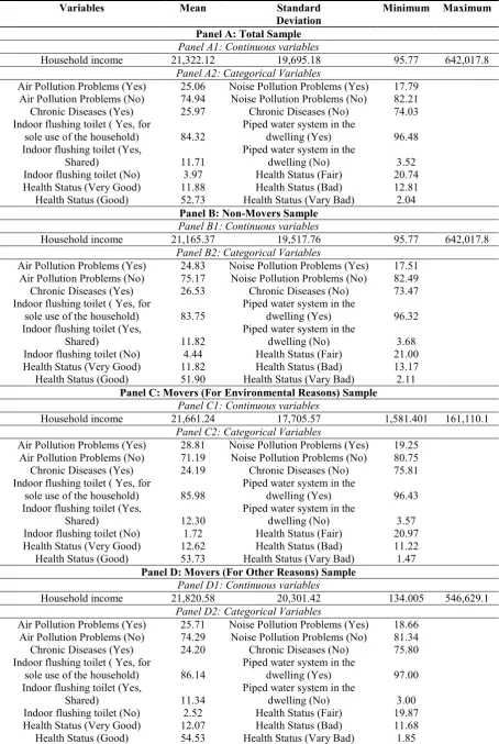
In table 1 the summary statistics for four different samples are reported. The average

household income is around 21,300 Turkish Liras for the total sample, while the average is

slightly higher for movers. The self-reported responses for air and noise pollution complaints

are similar among all samples where the 25 and 17 per cent claim that there are problems about

air and noise pollution respectively, while the 75 and 82 per cent declares no problems.

The 25 per cent of the sample reports that it suffers from a chronic illness, while the rest 75

per cent declares no. The statistics show that almost all the households in the sample have

available piped water in the dwelling at 96 per cent. Regarding the self-reported health status

table 1 show that 11.88 and 52.73 per cent report very good and good health respectively, the

20.74 reports fair health status, while 12.81 and 2.04 per cent report respectively bad and very

bad health status. Non movers sample report a slightly higher proportion of bad health at 13.17

per cent, while the movers for environmental or other reasons, presented in panels C and D,

report slightly higher proportions of very good and good health, as well as, lower proportions

of bad and very bad health.

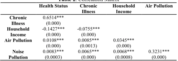
In table 2 the correlation matrix between household income, self-reported air and noise

pollution problems, the dummy whether an individual suffers from a chronic disease and the

self-reported ordered health status variable is presented. From table 2 the correlation between

household income and health status is negative indicating that the higher income is associated

with better health status, given that health status is very good for 1 and very bad for 5. Similarly,

the association between income and suffering from a chronic disease is negative. Noise and air

pollution are associated positively with poor health status and the probability that an individual

will report that he/she suffers from chronic disease. Chronic disease self-report is positively

correlated with poor health status, while income is positively associated with air and noise

pollution, probably indicating that individuals with higher income are located in more polluted

areas as urban areas.

In addition, the correlation between temperature and health status is -0.0151, while between

temperature and chronic illness is -0.0116. Similarly the correlation of wind speed with health

status and chronic illness is 0.0037 and 0.0034 respectively, while the respective values for

humidity are 0.0072 and 0.0025. These results are reported as an additional regression using

weather data for non-movers sample takes place.

(Tables 1-2 around here)

5. Empirical Results

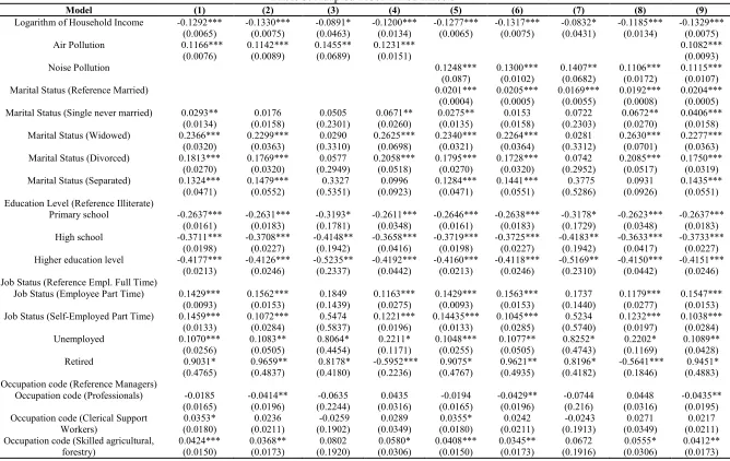
In this section the estimation results are presented and discussed. Equation (10) is estimated

adapted Probit-OLS estimates are presented. It should be noticed that a negative sign is

associated with better health outcome levels, as the self-reported health status variable is

defined as 1 for very good health and 5 for very bad health status. The self-reported air and

noise complaint present the expected positive signs, while income’s coefficient sign is negative

respectively. Therefore a rise in air pollution increases the probability of health status

deterioration occurrence. In table 3 the estimates are provided for fours samples; the total

sample; the non-movers sample; the movers for environmental reasons movers and the movers

for other reasons sample.

Income has a negative sign indicating that the higher income is associated with higher-better

levels of health outcome. Richer people who are better educated have better health status levels

than poorer, who are usually less-educated people. In addition people with higher income have

access to better quality of housing, schooling, and nutrition (Deaton, 2001).

The role of education in health status is key determinants of health and living standards.

Moreover, an individual’s health and well-being are partly determined by their life-cycle

experience and by the social roles and class - in terms of marital status, employment, parenthood

status - and less by other household characteristics as fuel type used, pipe water infrastructure,

while house tenure has no significant effects. Therefore, those who are single (never married)

report lower levels of health status followed by separated and divorced individuals. Those who

are widowed present the lowest health outcome levels amongst the other categories of marital

status. Regarding education level, the reference category is the illiterate individuals. It becomes

clear that higher education levels are associated with higher levels of health outcome. For

example individuals who have completed the primary school report a better health outcome by

0.301, while those who have completed high school and higher education are healthier by 0.449

and 0.518 respectively. Similarly, job status is an important determinant of health status. The

unemployed and retired individuals indicates a lower level of health status for these categories

than for people who are full-time employed. Especially, the retired and widowed people present

the lowest levels of health status, reflecting their old age which implies additional health

problems. More specifically, more than 40 per cent of the widowed individuals are older than

55 years old. In table 3 the results for occupation codes are reported. More specifically, there is

no difference on health status between individuals who are professionals and the reference

category which is managers. However, skilled workers employed in agricultural and forestry

industry present lower levels of health outcomes followed by clerical support workers.

Regarding household type the results are mixed. Another possible factor could be used in this

case is the household size, or number of children. However, the former factor allows us to

examined more detailed the effects and structure of a household, rather than taking only the

size. More specifically, from table 3 it becomes clear that a couple younger than 65 years old

with no dependent children and are healthier than a household which is consisted only by a

single person. Similarly a household, which is consisted by two adults with one or two

dependent children, present higher levels of health status than single individuals. These findings

are also captured by the marital status. On the other hand, a household, which is consisted by

two adults with no dependent children, but at least one of them is older than 65 years old, are

less healthy than single persons, which reflects the old age of those persons, as in the case of

widowed and retired people. Previous studies show evidence on the protective and beneficial

role of family size and support to individuals’ health outcomes (Aldwin and Greenberger, 1987;

Doornbos, 2001). Therefore, household type and support can be proxies to home health care

indicating this type of care may substitute the medical care obtained in the market which

improves individuals’ health leaving in supporting and big families.

Generally, the results overall show that education is perhaps the most basic socio-economic

future labour market opportunities and earning potentials. Moreover, education provides

knowledge and life skills that allow persons to gain more access to information and resources

to health services and care. The general findings so far are consistent with other studies

(Benzeval et al., 2000; Prus, 2001; Robert and Li 2001; Deaton, 2001; Beckett and Elliott, 2002;

Bostean, 2010).

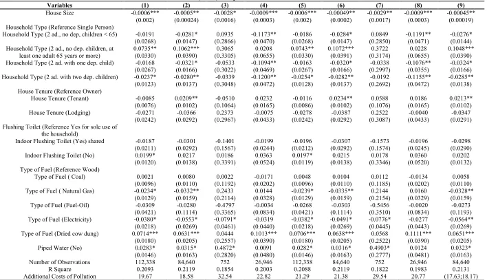
The rest of the factors have small or insignificant effects on health. More specifically, house

tenure is insignificant, with the exception the movers for other reasons sample where the tenants

have lower health level than the owners. This reflects two things; the owners are either

individuals with higher income or are supported by the household. The rest of the determinants

examined is the indoor flushing toilet and piped water in the dwelling and the type of fuel used

for healing. This is the first study which explores these factors, which based on the estimate are

important determinants of health status. Table 3 shows that whether there is indoor flushing

toilet for sole use of the household or shared has no different impact on health; however, the

individuals who answered that there is no indoor flushing toilet and no piped water in the

dwelling have lower health status levels. Finally, the type of fuel used for heating in the

dwelling is important for the health status. More specifically, either using wood or coal has no

difference on health; however using natural gas, fuel-oil and electricity has more positive effects

on individuals’ health status than coal or wood. In addition, when dried cow dung is used as

fuel for heating has significant negative effects on health status.

Based on table 3 the additional costs for air and noise pollution are reported. Respondents

who reported that there is problem with air pollution face an additional cost of air pollution

impact equal at 19.67 TL per month for total sample, 18.58 TL for the non-movers sample,

32.54 TL for the movers for environmental reasons movers and 22.82 TL concerning the

movers for other reasons sample. The respective additional costs for noise pollution impact is

movers for environmental reasons movers and 20.77 TL based on columns (5)-(8) of table 3.

Therefore, individuals who moved because of environmental or other reasons evaluate more

the air pollution than noise, while the additional costs for non-movers sample are similar with

those derived using the total sample. This can be explained by the fact that 76 per cent of the

survey is non-movers.

(Table 3 around here)

The next tables 4-6 present different econometric models for the health status and the

analysis is restricted to non-movers in order to limit possibly endogeneity. In table 4 the

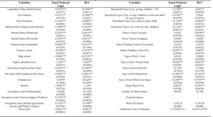
estimates using panel ordered Logit and BUC estimates are reported. The results confirm the

findings described previously for the table 3 and the adapted Probit fixed effects estimates. The

coefficients have the same sign, while the magnitude is higher as these methods use the Logit

approach where the coefficients are roughly 4 times higher than the coefficients derived from

the linear regression. Moreover, the additional costs in table 3 are very similar with those in

table 4 discussed previously.

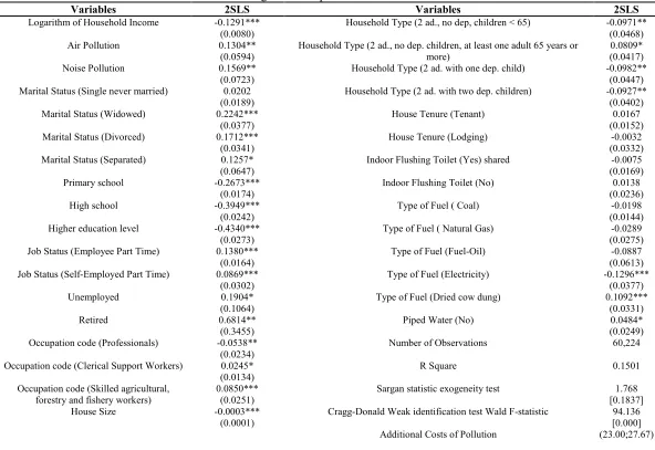
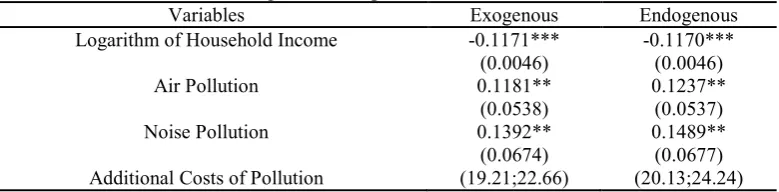
In tables 5-6 the results for the two and three stage least squares respectively are reported.

The sign and the impact of the various determinants on health is similar with the previous results

confirming the estimates and the importance of each factor on health. However, the additional

costs in tables 5-6 are higher. More specifically, regarding the two stage least squares estimates

the additional costs of air and noise pollution are 23.00 TL and 27.67 TL per month, while in

the case of the adapted Probit fixed effects in table 3 and column (9) the respective additional

costs are 17.63 TL and 18.17 TL. This indicates that the estimates of the fixed effects model in

table 4 are biased downward and the additional costs are underestimated. Similarly, the

and equal at 20.13 TL and 24.24 TL per month, when instruments are used. In addition, when

the self-reported air and noise pollution problems are considered as exogenous are still higher

than the fixed effects model and the individuals face additional costs equal at 19.21 TL and

12.66 TL per month than the individuals who do not report any complain or problem with air

and noise pollution. However, the additional costs, using three stage least squares, are slightly

lower than those calculated based on the two stage least squares. Nevertheless, as it has been

discussed in the methodology section, the former approach can be more robust for two reasons.

Firstly, it is not precise to calculate additional costs and to disentangle the effects of air and

noise pollution when both self-reported complains about environment are used in the

regression. Secondly, there is a strong possibility that the error term between the two equations,

one for each pollution question, is correlated therefore the three stage least squares method is

more appropriate in this case. Generally, in rural areas the air and noise pollution has significant

effects too. This can be explained by the fact that modern farms using noise equipment has

replaced the old-fashioned farming type (Aecom, 2011; Ovenden et al., 2011). Also one major

source of noise is traffic which comes especially from freeways, but it is also dominated in the

centres of big cities. In any case since noise depends on the wind direction and speed, one

plausible action of reducing the noise pollution is the construction of noise barriers next to the

freeways.

(Tables 4-6 around here)

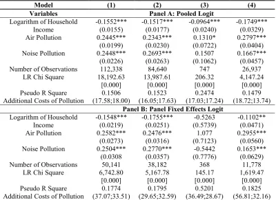
The next step is to present the results for chronic illnesses. More specifically, the results

regarding the effects of income and air-noise pollution on chronic illness probability occurrence

are reported in table 7. In panel A the estimates using a pooled binary Logit model are reported,

previously. The additional costs in panel A range between 16.00-18.00 TL per month, while

the additional costs of noise pollution reduction are 13.74 per month in the movers for other

reasons sample in column (4). However, in panel B the additional costs are significantly higher,

almost doubled, than in panel A, showing the biases derived by pooled estimates. Moreover,

the estimates using an instrumental binary Probit model with random effects, using the regional

complaint rates and wind direction as instruments, took place where the additional costs are

similar with those derived from fixed effects Logit data. The coefficients for the rest of the

health status determinants are not reported as the concluding remarks are similar with those

derived previously for the health status. However, what it is important is the additional costs;

where in case of the individuals who suffer from specific chronic diseases are significantly

higher.

Finally, in table 7 additional estimates are reported in order to calculate the first and the

third term of equation (8). The estimates in panel A of table 8 show the effect of poor health

status and chronic diseases on working hours lost. Individuals with poor health status on

average work less by 1.3 and 1.5 hours than people with good health status for the total and

non-movers sample. In addition, higher household income is associated with lower hours of

work. Similarly, the individuals who suffer from chronic illness are working less by 1.3 hours

than people who do not suffer. However, this does not imply that working hours lost is

associated with avoidance behaviour. Nevertheless, one assumption is that individuals with

poor health status might avoid attending work in order to avoid high outdoor pollution level. At

the same time the estimates in panel A can be used in order calculate the third term

(∂M/∂E)(PM), where the assumption of visiting a practitioner or hospital can be examined. In

that case the PM can be considered as zero because the hospital services in Turkey are free, if

the exclusion of private services is assumed, which is not the main scope of the study but these

is taken here as an example, which included the transportation time and list queuing time for

visiting a practitioner. Therefore, the third term is equal 3.9 and 4.5 less working hours for

individuals with poor health status relatively to those with good health status.

Finally, the first term of equation (8) (∂w/∂H)(dH/dE) using the estimates from table 11 and

panel B, as well as the estimates from table 3 and column (9), can be calculated. The term

(∂w/∂H)(dH/dE) it is equal at 1.25 and 1.39 per cent for air and noise pollution respectively

and non-movers with poor health status. Similarly, for the individuals who suffer from chronic

diseases the cost is 0.92 and 1.02 per cent for air and noise respectively. Using the three stage

least squares estimates from table 8 and column (2) -which are 0.1237 and 0.1489 per cent for

air and noise pollution respectively- (∂w/∂H)(dH/dE) is equal at 1.47 and 1.77 per cent for air

and noise pollution respectively, while the respective values for individuals who suffer from

chronic illness are 1.08 and 1.31 per cent. Thus, individuals with poor health earn wage less by

1.5-1.8 per cent cause by air and noise pollution, while the respective reduction in wage for

individuals who suffer from chronic illness is 1.08 and 1.31 caused by air and noise pollution

respectively.

(Tables 7-8 around here)

Overall, the results suggest that one of the main policies in Turkey should be education

reconstruction, health promotion and income distribution focusing on SES disparities

elimination and reducing income inequalities on health. Furthermore, a broad approach to the

multiple determinants of SES disparities in health should be reduced or not eliminated.

Therefore a new approach is needed in policy circles that would reconsider the benefit side of

the cost-benefit analysis. Traditionally, these calibrations emphasize economic efficiency or

cost-saving, prospects of policies that improve education or equalize resources. Finally, the results

confirm the proposal by International Energy Agency (2010), which suggests that Turkey

should promote fuel switching from high-sulphur lignite and coal to natural gas.

However, there are some drawbacks in this study. Firstly, the econometric methods applied

as well as the relationship between health, pollution and other socioeconomic and demographic

factors, seemingly require the availability of panel data. Therefore, one of the most important

limitations the repeated cross-sectional data is that it is impossible to follow the same

individuals across the time period examined. Nevertheless, repeated cross-sectional data suffer

less from the typical problems of non-response and attrition presented in the panel data surveys.

These problems can be significantly larger with increases in the number of units i.e. individuals,

households or firms.

Moreover, there is additional information on whether the individuals or household have

changed address during the last five years limiting in this way the endogeneity problem and

examining different samples based on their moving status. Finally, another very important

factor which is the main consideration in the epidemiological studies is the “unobservable”

characteristics of the individuals, which are inherited at birth or genetic and that may influence

the health outcomes. Ignoring these characteristics the association between income and health

might not represent the true relationship. However, it is very difficult or even impossible to find

appropriate variables or measures to use them as proxies for such characteristics including this

survey.

Furthermore, other approaches such as Generalized Ordered Probit or Logit Latent Class

models can be applied in order to account for slope heterogeneity, while robustness checks for

6. Conclusions

This study has used a set of repeated cross sectional and pseudo panel micro-data on

self-reported health status, chronic illness and air-noise pollution from the Income and Living

Conditions Survey in Turkey. Various econometric approaches have been applied for

robustness checks. The results showed that the additional costs for the individual who report a

problem on air and noise pollution are higher by 22-25 TL per month than the individuals who

did not report. In addition, most of the determinants examined in this study have significant

effects on health status, with education to be the most important one followed by job status,

marital status, house size and household type. House tenure shows no significant effects on

health, while this study examines additional determinants than other studies, such as piped

water, indoor flushing toilet and type of fuel for heating effects on health. Moreover, various

cases have been examined in, as the urban versus rural areas, gender and age groups. Finally,

the costs effects of air and noise pollution on wage and working hours lost because of illness

have been examined.

References

Aecom (2011) Wind Farm Noise Statutory Nuisance Complaint Methodology. Report Prepared for Defra. Contract No. NANR 277.

Aldwin C, Greenberger E (1987) Cultural differences in the predictors of depression. American J Community Psychol 15(6): 789-813.

Baetschmann G, Staub KE, Winkelmann R (2014) Consistent Estimation of the Fixed Effects Ordered Logit Model. J R Stat Soc Ser A-G 178(3): 685-703.

Beckett M, Elliott MN (2002) Does the Association Between Marital Status and Health Vary by Sex, Race, and Ethnicity? Rand, Labor and Population Program. Working Paper Series 02-08.

Benzeval M, Taylor J, Judge K (2000) Evidence on the relationship between low income and poor health: Is the Government doing enough? Fisc Stud 21(3):375-399.

Bostean G (2010) An Examination of the Relationship between Family and U.S. Latinos’ Physical Health. Field Actions Science Reports. Migr Health 2: 1-7.

Chay KY, Greenstone M (2003a) Air Quality, Infant Mortality, and the Clean Air Act of 1970. NBER Working Paper No. 10053, Cambridge, MA.

Chay KY, Greenstone M (2003b) The Impact of Air Pollution on Infant Mortality: Evidence from Geographic Variation in Pollution Shocks Induced by a Recession. Q J Econ 118(3):1121-1167.

Currie J, Neidell M (2005) Air Pollution and Infant Health: What Can We Learn from California's Recent Experience? Q J Econ 120(3):1003-1030.

Deaton A (1985) Panel Data from Time Series of Cross Sections. J Econometrics, 30(1-2): 109-126.

Deaton A (2001) Inequalities in Income and Inequalities in Health. In Welch, F. ed. The causes and consequences of increasing inequality. Chicago: Chicago University Press.

Delfino RJ, Murphy-Moulton AM Becklake MR (1998) Emergency room visits for respiratory illnesses among the elderly in Montreal: association with low level ozone exposure. Environ Res Sec A 76(2): 67 – 77.

Dockery D, Pope CA, Xiping X, Spengler J, Ware J, Fay M, Ferris B, Speizer F (1993) An Association between Air Pollution and Mortality in Six U.S. Cities. New Enlg J Med 329(24):1753–1759.

Doornbos MM (2001) Professional support for family care-givers of people with serious and persistent mental illnesses. J Psychosoc Nursing 39(12):38-45

Doygun H, Gurun DK (2008) Analysing and mapping spatial and temporal dynamics of urban traffic noise pollution: a case study in Kahramanmaras, Turkey. Environ Monit Assess142(1-3) :65-72.

Erdogan E, Yazgan M (2009) Landscaping in reducing traffic noise problem in cities: Ankara case. Afric J Agric Res 4(10):1015-1022.

Ferrer-i-Carbonell A, Frijters P (2004) How important is Methodology for the estimates of the determinants of Happiness? Econ J 114(497):641-659.

Fraser H, Eng P (2012) Understanding and Reducing Noise Nuisance From Stationary Farm Equipment.. Order N. 12-029 AGDEX 700

Gerking S, Stanley RL (1986) An Economic Analysis of Air Pollution and Health: The Case of St. Louis. Rev Econ Stat 68(1):115-121.

Greene W (2011) Econometric Analysis. Seventh Edition. Upper Saddle River, New Jersey: Prentice Hall.

Griefahn B (2002) Sleep disturbances related to environmental noise. Noise Health 4(15):57-60.

International Energy Agency (2010) Energy Policies of IEA Countries, Turkey 2009 Review. Janssen NAH, Schwartz J, Zanobetti A, Suh HH (2002) Air conditioning and source-specific

particles as modifiers of the effect of PM10 on hospital admissions for heart and lung disease. Environ Health Persp 110(1):43 – 49.

Laden F, Neas LM Dockery DW, Schwartz J (2000) Association of fine particulate matter from different sources with daily mortality in six US cities. Environ Health Persp 108(10):941 – 947.

Luechinger S (2009) Valuing Air Quality Using the Life Satisfaction Approach. Econ J 119(536):482-515.

Murray MP (2006) Avoiding Invalid Instruments and coping with weak Instruments. J Econ Perspect 20(4): 111-132.

Naeher LP, Holford, TR, Beckett WS Belanger K, Triche EW, Bracken MB et al (1999) Healthy Women’s PEF Variations with Ambient Summer Concentrations of PM10, PM2.5, SO4-2, H+,

and O3. Am J Resp Crit Care 160(1):117–125.

Okuguchi T, Osanai T, Fujiwara N, Kato T, Metoki N, Konta Y, Okumura K (2002) Effect of losartan on nocturnal blood pressure in patients with stroke: comparison with angiogenesis converting enzyme inhibitor. Am J Hypertens 15(11):998-1002.

O’Neill MS, Loomis D, Borja-Aburto VH (2004) Ozone, area social conditions, and mortality in Mexico City. Environ Res 94(3):234–242.

Ovenden N, Shaffer S, Fernando H (2011) How the weather affects the scale of urban noise pollution. Popular version of paper 2pNS3. Presented Tuesday Afternoon, May 24, 2011, 161st Acoustical Society of America Meeting, Seattle, Wash.

Ozer S, Yilmaz H Yesil M, Yesil P (2009) Evaluation of noise pollution caused by vehicles in the city of Tokat, Turkey. Sci Res Essays 4(11):1205-1212.

Ozyonar F, Peker I (2008) ‘Investigation of the environmental noise pollution in Sivas City Centre. Ecology, 18(69):75-80.

Preutthipan A, Udomsubpayakul, U, Chaisupamongkollarp, T, Pentamwa, P (2004) Effect of PM10 pollution in Bangkok on Children with and without asthma. Pediatr Pulm 37(3):187 – 192.

Prus GS (2001) The Relationship between Age, Socio-Economic Status, and Health among Adult Canadians. Social and Economics Dimensions of An Ageing Population. SEDAP Research Paper No. 57.

Robert AS, Li WL (2001) Age Variation in the Relationship Between Community Socioeconomic Status and Adult Health. Res Aging 23(2):233-258.

Sisman EE, Unver E (2011) Evaluation of traffic noise pollution in Corlu, Turkey. Sci Res Essays 6(14):3027-3033.

Tanrıvermiş H (1998) Willingness to Pay WTP and Willingness to Accept WTA Measures in Turkey: May WTP and WTA Be Indicators to Share the Environmental Damage Burdens: A Case Study. J. Econ. Cooperation Islamic Countries 19(3):67-93.

Tekeşin C, Shihomi A (2014) Measuring the Value of Mortality Risk Reductions in Turkey. Int

J Environ Res Public Health 11(7):6890-6922.

Turkish Statistical Institute (2013) Income and Living Conditions Survey Micro Data Set Cross Sectional, 2006-2012. Ankara.

Yilmaz H, Ozer S (2005) Evaluation and analysis of environmental noise pollution in the city of Erzurum, Turkey. Int. J. Environ Poll 23(4):438-448.

Van Praag B, Ferrer-i-Carbonell A (2004) Happiness quantified: A satisfaction calculus approach. Oxford: Oxford University Press.

Van Praag B, Ferrer-i-Carbonell A (2006) An almost integration-free approach to ordered response models. Tinbergen Institute Discussion Paper TI 2006-047/3.

Zellner A (1962) An efficient method of estimating seemingly unrelated regression equations and tests for aggregation bias. J Am Stat Assoc 57(298):348-368.

Table 1. Summary Statistics

Variables Mean Standard

Deviation

Minimum Maximum

Panel A: Total Sample

Panel A1: Continuous variables

Household income 21,322.12 19,695.18 95.77 642,017.8 Panel A2: Categorical Variables

Air Pollution Problems (Yes) 25.06 Noise Pollution Problems (Yes) 17.79 Air Pollution Problems (No) 74.94 Noise Pollution Problems (No) 82.21 Chronic Diseases (Yes) 25.97 Chronic Diseases (No) 74.03 Indoor flushing toilet ( Yes, for

sole use of the household) Indoor flushing toilet (Yes,

Shared)

Indoor flushing toilet (No) Health Status (Very Good)

Health Status (Good)

84.32

11.71 3.97 11.88 52.73

Piped water system in the dwelling (Yes) Piped water system in the

dwelling (No) Health Status (Fair) Health Status (Bad) Health Status (Vary Bad)

96.48

3.52 20.74 12.81 2.04 Panel B: Non-Movers Sample

Panel B1: Continuous variables

Household income 21,165.37 19,517.76 95.77 642,017.8 Panel B2: Categorical Variables

Air Pollution Problems (Yes) 24.83 Noise Pollution Problems (Yes) 17.51 Air Pollution Problems (No) 75.17 Noise Pollution Problems (No) 82.49 Chronic Diseases (Yes) 26.53 Chronic Diseases (No) 73.47 Indoor flushing toilet ( Yes, for

sole use of the household) Indoor flushing toilet (Yes,

Shared)

Indoor flushing toilet (No) Health Status (Very Good)

Health Status (Good)

83.75

11.82 4.44 11.82 51.90

Piped water system in the dwelling (Yes) Piped water system in the

dwelling (No) Health Status (Fair) Health Status (Bad) Health Status (Vary Bad)

96.32

3.68 21.00 13.17 2.11 Panel C: Movers (For Environmental Reasons) Sample

Panel C1: Continuous variables

Household income 21,661.24 17,705.57 1,581.401 161,110.1 Panel C2: Categorical Variables

Air Pollution Problems (Yes) 28.81 Noise Pollution Problems (Yes) 19.25 Air Pollution Problems (No) 71.19 Noise Pollution Problems (No) 80.75 Chronic Diseases (Yes) 24.19 Chronic Diseases (No) 75.81 Indoor flushing toilet ( Yes, for

sole use of the household) Indoor flushing toilet (Yes,

Shared)

Indoor flushing toilet (No) Health Status (Very Good)

Health Status (Good)

85.98

12.30 1.72 12.62 53.73

Piped water system in the dwelling (Yes) Piped water system in the

dwelling (No) Health Status (Fair) Health Status (Bad) Health Status (Vary Bad)

96.43

3.57 20.97 11.22 1.47 Panel D: Movers (For Other Reasons) Sample

Panel D1: Continuous variables

Household income 21,820.58 20,301.42 134.005 546,629.1 Panel D2: Categorical Variables

Air Pollution Problems (Yes) 25.71 Noise Pollution Problems (Yes) 18.66 Air Pollution Problems (No) 74.29 Noise Pollution Problems (No) 81.34 Chronic Diseases (Yes) 24.20 Chronic Diseases (No) 75.80 Indoor flushing toilet ( Yes, for

sole use of the household) Indoor flushing toilet (Yes,

Shared)

Indoor flushing toilet (No) Health Status (Very Good)

Health Status (Good)

86.14

11.34 2.52 12.07 54.53

Piped water system in the dwelling (Yes) Piped water system in the

dwelling (No) Health Status (Fair) Health Status (Bad) Health Status (Vary Bad)

97.00

Table 2. Correlation Matrix Health Status Chronic

Illness

Household Income

Air Pollution

Chronic Illness

0.6514*** (0.000) Household

Income

-0.1427*** (0.000)

-0.0755*** (0.000) Air Pollution 0.0108***

(0.000)

0.0085*** (0.0013)

0.0345*** (0.000) Noise

Pollution

0.0083*** (0.0003)

0.0065*** (0.000)

0.0068*** (0.0008)

Table 3. Adapted Probit Fixed Effects

Model (1) (2) (3) (4) (5) (6) (7) (8) (9)

Logarithm of Household Income -0.1292*** (0.0065) -0.1330*** (0.0075) -0.0891* (0.0463) -0.1200*** (0.0134) -0.1277*** (0.0065) -0.1317*** (0.0075) -0.0832* (0.0431) -0.1185*** (0.0134) -0.1329*** (0.0075) Air Pollution 0.1166***

(0.0076) 0.1142*** (0.0089) 0.1455** (0.0689) 0.1231*** (0.0151) 0.1082*** (0.0093)

Noise Pollution 0.1248***

(0.087) 0.1300*** (0.0102) 0.1407** (0.0682) 0.1106*** (0.0172) 0.1115*** (0.0107) Marital Status (Reference Married) 0.0201***

(0.0004) 0.0205*** (0.0005) 0.0169*** (0.0055) 0.0192*** (0.0008) 0.0204*** (0.0005) Marital Status (Single never married) 0.0293**

(0.0134) 0.0176 (0.0158) 0.0505 (0.2301) 0.0671** (0.0260) 0.0275** (0.0135) 0.0153 (0.0158) 0.0722 (0.2303) 0.0672** (0.0270) 0.0406*** (0.0158) Marital Status (Widowed) 0.2366***

(0.0320) 0.2299*** (0.0363) 0.0290 (0.3310) 0.2625*** (0.0698) 0.2340*** (0.0321) 0.2264*** (0.0364) 0.0281 (0.3312) 0.2630*** (0.0701) 0.2277*** (0.0363) Marital Status (Divorced) 0.1813***

(0.0270) 0.1769*** (0.0320) 0.0577 (0.2949) 0.2058*** (0.0518) 0.1795*** (0.0270) 0.1728*** (0.0320) 0.0742 (0.2952) 0.2085*** (0.0517) 0.1750*** (0.0319) Marital Status (Separated) 0.1324***

(0.0471) 0.1479*** (0.0552) 0.3327 (0.5351) 0.0996 (0.0923) 0.1284*** (0.0471) 0.1441*** (0.0551) 0.3775 (0.5286) 0.0931 (0.0926) 0.1435*** (0.0551) Education Level (Reference Illiterate)

Primary school -0.2637*** (0.0161) -0.2631*** (0.0183) -0.3193* (0.1781) -0.2611*** (0.0348) -0.2646*** (0.0161) -0.2638*** (0.0183) -0.3178* (0.1729) -0.2623*** (0.0348) -0.2637*** (0.0183) High school -0.3711***

(0.0198) -0.3708*** (0.0227) -0.4148** (0.1942) -0.3658*** (0.0416) -0.3719*** (0.0198) -0.3725*** (0.0227) -0.4183** (0.1942) -0.3633*** (0.0417) -0.3733*** (0.0227) Higher education level -0.4177***

(0.0213) -0.4126*** (0.0246) -0.5235** (0.2337) -0.4192*** (0.0442) -0.4160*** (0.0213) -0.4118*** (0.0246) -0.5169** (0.2310) -0.4150*** (0.0442) -0.4151*** (0.0246) Job Status (Reference Empl. Full Time)

Job Status (Employee Part Time) 0.1429*** (0.0093) 0.1562*** (0.0153) 0.1849 (0.1439) 0.1163*** (0.0275) 0.1429*** (0.0093) 0.1563*** (0.0153) 0.1737 (0.1440) 0.1179*** (0.0277) 0.1547*** (0.0153) Job Status (Self-Employed Part Time) 0.1459***

(0.0133) 0.1072*** (0.0284) 0.5474 (0.5837) 0.1221*** (0.0196) 0.14435*** (0.0133) 0.1045*** (0.0285) 0.5234 (0.5740) 0.1232*** (0.0197) 0.1038*** (0.0284) Unemployed 0.1070***

(0.0256) 0.1083** (0.0505) 0.8064* (0.4454) 0.2211* (0.1171) 0.1048*** (0.0255) 0.1077** (0.0505) 0.8252* (0.4743) 0.2202* (0.1169) 0.1089** (0.0428) Retired 0.9031*

(0.4765) 0.9659** (0.4837) 0.8178* (0.4180) -0.5952*** (0.2236) 0.9075* (0.4767) 0.9621** (0.4935) 0.8196* (0.4182) -0.5641*** (0.1846) 0.9451* (0.4883) Occupation code (Reference Managers)

Occupation code (Professionals) -0.0185 (0.0165) -0.0414** (0.0196) -0.0635 (0.2244) 0.0435 (0.0316) -0.0194 (0.0165) -0.0429** (0.0196) -0.0744 (0.216) 0.0448 (0.0316) -0.0435** (0.0195) Occupation code (Clerical Support

Workers) 0.0353* (0.0180) 0.0236 (0.0211) -0.0259 (0.1902) 0.0289 (0.0349) 0.0355* (0.0180) 0.0242 (0.0211) -0.0243 (0.1913) 0.0271 (0.0349) 0.0217 (0.0211) Occupation code (Skilled agricultural,

Table 3 (cont.) Adapted Probit Fixed Effects

Variables (1) (2) (3) (4) (5) (6) (7) (8) (9)

House Size -0.0006*** (0.002) -0.0005** (0.00024) -0.0028* (0.0016) -0.0009*** (0.0003) -0.0006*** (0.002) -0.00049** (0.0002) -0.0029** (0.0017) -0.0009*** (0.0003) -0.00045** (0.00019) Household Type (Reference Single Person)

Household Type (2 ad., no dep, children < 65) -0.0191 (0.0268) -0.0281* (0.0147) 0.0935 (0.2866) -0.1173** (0.0470) -0.0186 (0.0268) -0.0284* (0.0147) 0.0849 (0.2850) -0.1191** (0.0471) -0.0276* (0.0144) Household Type (2 ad., no dep. children, at

least one adult 65 years or more)

0.0735** (0.0330) 0.1062*** (0.0390) 0.3065 (0.3305) 0.0208 (0.0655) 0.0743** (0.0330) 0.1072*** (0.0391) 0.3722 (0.3174) 0.0228 (0.0655) 0.1048*** (0.0390) Household Type (2 ad. with one dep. child) -0.0168

(0.0267) -0.0321* (0.0166) -0.0533 (0.3022) -0.1094** (0.0469) -0.0163 (0.0267) -0.0320* (0.0166) -0.0338 (0.2997) -0.1076** (0.0355) -0.0324* (0.0166) Household Type (2 ad. with two dep. children) -0.0237*

(0.0123) -0.0280** (0.0137) -0.0339 (0.3048) -0.1200** (0.0472) -0.0254* (0.0128) -0.0282** (0.0137) -0.0192 (0.2692) -0.1155** (0.0472) -0.0285** (0.0138) House Tenure (Reference Owner)

House Tenure (Tenant) -0.0085 (0.0076) 0.0209** (0.0102) -0.0510 (0.1064) 0.0232 (0.0165) -0.0116 (0.0086) 0.0234** (0.0102) 0.0588 (0.1076) 0.0186 (0.0165) 0.0213** (0.0102) House Tenure (Lodging) -0.0271

(0.0242) -0.0366 (0.0292) 0.2373 (0.2967) -0.0075 (0.0433) -0.0278 (0.0242) -0.0387 (0.0292) 0.2522 (0.3087) -0.0040 (0.0433) -0.0347 (0.0291) Flushing Toilet (Reference Yes for sole use of

the household)

Indoor Flushing Toilet (Yes) shared -0.0187 (0.0211) -0.0301 (0.0292) -0.1401 (0.1567) -0.0199 (0.0244) -0.0196 (0.0212) -0.0307 (0.0292) -0.1573 (0.1574) -0.0196 (0.0245) -0.0298 (0.0290) Indoor Flushing Toilet (No) 0.0199*

(0.0120) 0.0217 (0.0138) 0.0186 (0.3391) 0.0363 (0.0524) 0.0197* (0.0119) 0.0215 (0.0138) 0.0178 (0.3346) 0.0360 (0.0520) 0.0202 (0.0132) Type of Fuel (Reference Wood)

Type of Fuel ( Coal) 0.0021 (0.0096) 0.0080 (0.0110) 0.0022 (0.1192) -0.0171 (0.0202) 0.0048 (0.0096) 0.0104 (0.0110) 0.0112 (0.1185) -0.0134 (0.0202) 0.0058 (0.0110) Type of Fuel ( Natural Gas) -0.0234*

(0.0129) -0.0332** (0.0159) 0.2433 (0.2114) 0.0144 (0.0328) -0.0239* (0.0129) -0.0335** (0.0159) 0.2144 (0.2154) 0.0160 (0.0329) -0.0328** (0.0159) Type of Fuel (Fuel-Oil) -0.0309

(0.0421) -0.0280 (0.1114) -0.4797 (0.3365) -0.0034 (0.0834) -0.0268 (0.0421) -0.0303 (0.1114) -0.5456 (0.3510) -0.0020 (0.0834) -0.0273 (0.1193) Type of Fuel (Electricity) -0.0380*

(0.0218) -0.0553* (0.0269) -0.0791* (0.0461) -0.0319 (0.0440) -0.0382* (0.0218) -0.0491* (0.0269) -0.0776* (0.0445) -0.0277 (0.0443) -0.0564** (0.0269) Type of Fuel (Dried cow dung) 0.0714***

(0.0180) 0.0631*** (0.0205) 0.0444 (0.2557) 0.1013*** (0.0390) 0.0706*** (0.0180) 0.0638*** (0.0205) 0.0568 (0.2522) 0.1111*** (0.0390) 0.0651*** (0.0205) Piped Water (No) 0.0283*

(0.0146) 0.0315* (0.0163) 0.4872* (0.2820) 0.0091 (0.0480) 0.0282* (0.0146) 0.0316* (0.0163) 0.4903* (0.2777) 0.0124 (0.0481) 0.0323* (0.0163) Number of Observations 112,338 84,640 752 26,946 112,338 84,640 752 26,946 84,640

R Square 0.2093 0.2119 0.1854 0.2003 0.2088 0.2119 0.1822 0.1983 0.2131 Additional Costs of Pollution 19.67 18.58 32.54 22.82 21.29 21.38 29.54 20.77 (17.63;18.17)

Table 4. Ordered Logit and BUC Models for Non-Movers Variables Panel Ordered

Logit

BUC Variables Panel Ordered

Logit

BUC

Logarithm of Household Income -0.2924*** (0.0137)

-0.3444*** (0.0211)

Household Type (2 ad., no dep, children < 65) -0.1350** (0.0673)

-0.0417* (0.0238) Air Pollution 0.2121***

(0.0178)

0.2360*** (0.0267)

Household Type (2 ad., no dep. children, at least one adult 65 years or more)

0.2194*** (0.0759)

0.2041 (0.2076) Noise Pollution 0.2382***

(0.0204)

0.2960*** (0.0302)

Household Type (2 ad. with one dep. child) -0.1359** (0.0676)

-0.0462** (0.0215) Marital Status (Single never married) 0.1990***

(0.0250)

0.1418*** (0.0496)

Household Type (2 ad. with two dep. children) -0.1335** (0.0673)

-0.0453** (0.0221) Marital Status (Widowed) 0.5251***

(0.0637)

0.6434*** (0.0991)

House Tenure (Tenant) 0.0242 (0.0707)

0.0549** (0.0255) Marital Status (Divorced) 0.5565***

(0.0576)

0.5017*** (0.0884)

House Tenure (Lodging) -0.0903 (0.0619)

-0.0825 (0.0866) Marital Status (Separated) 0.6039***

(0.1033)

0.5114*** (0.1546)

Indoor Flushing Toilet (Yes) shared -0.0143 (0.0376)

-0.0575 (0.0621) Primary school -0.6769***

(0.0282)

-0.5379*** (0.0477)

Indoor Flushing Toilet (No) 0.0722*** (0.0245)

0.0659* (0.0375) High school -0.9943***

(0.0385)

-0.8715*** (0.0622)

Type of Fuel ( Coal) 0.0161 (0.0199)

0.0400 (0.0298) Higher education level -1.165***

(0.0437)

-1.042*** (0.0688)

Type of Fuel ( Natural Gas) -0.0972** (0.0395)

-0.0676** (0.0357) Job Status (Employee Part Time) 0.3457***

(0.0253)

0.3540*** (0.0399)

Type of Fuel (Fuel-Oil) -0.1365 (0.1032)

-0.1606 (0.1579) Job Status (Self-Employed Part Time) 0.3645***

(0.0438)

0.2081*** (0.0751)

Type of Fuel (Electricity) -0.1926*** (0.0569)

-0.1623** (0.0793) Unemployed 0.3694*

(0.1884)

0.4228** (0.2059)

Type of Fuel (Dried cow dung) 0.1269*** (0.0342)

0.1978*** (0.0545) Retired 1.8682***

(0.0710)

1.210* (0.6164)

Piped Water (No) 0.0636* (0.0382)

0.1301** (0.0636) Occupation code (Professionals) -0.0368

(0.0428)

-0.1130* (0.0606)

Number of Observations 84,640 82,796

Occupation code (Clerical Support Workers) 0.1259*** (0.0429)

0.0837 (0.0626)

Pseudo R Square

Occupation code (Skilled agricultural, forestry and fishery workers)

0.1518*** (0.0338)

0.1140** (0.0480)

Wald Chi Square 7,528.34 [0.000]

6,756.20 [0.000] House Size -0.0013***

(0.00035)

-0.0013** (0.0005)

Additional Costs of Pollution (17.30;20.11) ((18.21;20.78)

Table 5. Two Stages Least Squares Estimates for Non-Movers

Variables 2SLS Variables 2SLS

Logarithm of Household Income -0.1291*** (0.0080)

Household Type (2 ad., no dep, children < 65) -0.0971** (0.0468) Air Pollution 0.1304**

(0.0594)

Household Type (2 ad., no dep. children, at least one adult 65 years or more)

0.0809* (0.0417) Noise Pollution 0.1569**

(0.0723)

Household Type (2 ad. with one dep. child) -0.0982** (0.0447) Marital Status (Single never married) 0.0202

(0.0189)

Household Type (2 ad. with two dep. children) -0.0927** (0.0402) Marital Status (Widowed) 0.2242***

(0.0377)

House Tenure (Tenant) 0.0167 (0.0152) Marital Status (Divorced) 0.1712***

(0.0341)

House Tenure (Lodging) -0.0032 (0.0332) Marital Status (Separated) 0.1257*

(0.0647)

Indoor Flushing Toilet (Yes) shared -0.0075 (0.0169) Primary school -0.2673***

(0.0174)

Indoor Flushing Toilet (No) 0.0138 (0.0236) High school -0.3949***

(0.0242)

Type of Fuel ( Coal) -0.0198 (0.0144) Higher education level -0.4340***

(0.0273)

Type of Fuel ( Natural Gas) -0.0289 (0.0275) Job Status (Employee Part Time) 0.1380***

(0.0164)

Type of Fuel (Fuel-Oil) -0.0887 (0.0613) Job Status (Self-Employed Part Time) 0.0869***

(0.0302)

Type of Fuel (Electricity) -0.1296*** (0.0377) Unemployed 0.1904*

(0.1064)

Type of Fuel (Dried cow dung) 0.1092*** (0.0331) Retired 0.6814**

(0.3455)

Piped Water (No) 0.0484* (0.0249) Occupation code (Professionals) -0.0538**

(0.0234)

Number of Observations 60,224

Occupation code (Clerical Support Workers) 0.0245* (0.0134)

R Square 0.1501

Occupation code (Skilled agricultural, forestry and fishery workers)

0.0850*** (0.0251)

Sargan statistic exogeneity test 1.768 [0.1837] House Size -0.0003***

(0.0001)

Cragg-Donald Weak identification test Wald F-statistic 94.136 [0.000] Additional Costs of Pollution (23.00;27.67)

32

Table 6. Three Stages Least Squares Estimates for Non-Movers

Variables Exogenous Endogenous Logarithm of Household Income -0.1171***

(0.0046)

-0.1170*** (0.0046) Air Pollution 0.1181**

(0.0538)

0.1237** (0.0537) Noise Pollution 0.1392**

(0.0674)

0.1489** (0.0677) Additional Costs of Pollution (19.21;22.66) (20.13;24.24)