Sparse Linear Models and l1−Regularized 2SLS with High Dimensional Endogenous Regressors and Instruments

Munich Personal RePEc Archive

Sparse Linear Models and l1Regularized

2SLS with High-Dimensional Endogenous

Regressors and Instruments

Zhu, Ying

Michigan State University

15 August 2013

Online at

https://mpra.ub.uni-muenchen.de/82184/

Sparse Linear Models and

l

₋

_{Regularized 2SLS with}

High-Dimensional Endogenous Regressors and Instruments

Ying Zhu

(Forthcoming in The Journal of Econometrics, October 2017)

Abstract

We explore the validity of the 2-stage least squares estimator with l₁₋regularization in both stages, for linear triangular models where the numbers of endogenous regressors in the main equation and instruments in the first-stage equations can exceed the sample size, and the regression coefficients are sufficiently sparse. For this l₁₋regularized 2-stage least squares esti-mator, we first establish finite-sample performance bounds and then provide a simple practical method (with asymptotic guarantees) for choosing the regularization parameter. We also sketch an inference strategy built upon this practical method.

JEL Classification: C14, C31, C36

Keywords: High-dimensional statistics; Lasso; sparse linear models; endogeneity; two-stage least squares

1

Introduction

The objective of this paper is consistent estimation of regression coefficients in models with a large number of endogenous regressors and instruments. We consider the linear model

Yi =Xiβ∗+ǫi = p

X

j=1

Xijβj∗+ǫi, i= 1, ..., n (1)

where ǫi is a zero-mean random error possibly correlated with Xi and β∗ is a vector of unknown

parameters of interest. The jth component ofβ∗ is denoted byβ_j∗.The jth component,Xij, of the

1×p vector, Xi, is endogenousifE(Xijǫi)6= 0, andexogenous ifE(Xijǫi) = 0.

When endogenous regressors are present, the classical least squares estimator will be inconsistent forβ∗ (i.e., ˆβOLS 9p β∗) even when the dimensionp of β∗ is fixed and small relative to the sample

size n. The two-stage least squares (2SLS) estimation plays an important role in accounting for endogeneity that comes from individual choice or market equilibrium (e.g., Wooldridge, 2010), and is based on the following “first-stage” equations for the components ofXi,

Xij =Zijπ∗j +ηij = dj

X

l=1

Zijlπjl∗ +ηij, i= 1, ...., n, j= 1, ..., p. (2)

For eachj= 1, ..., p,Zij is a 1×dj vector of instrumental variables,ηij a zero-mean random error

convenience, we will assume throughout the paper that all regressors in (1) are endogenous and dj = d ≥ (n∨2) in (2) for all j. Our primary interest concerns the regime where p ≥ (n∨2),

β∗ and π_j∗s are sufficiently sparse (meaning that the ordered coefficients in β∗ and π∗_j decay at sufficiently fast rates, which will be formalized in Section 2). The modification to allowp <(n_∨2) and/or dj 6=d_j′ forj6=j

′

is straightforward.

For statistical models where the dimension of parameters is comparable to or even larger than the sample size, regularization methods have been given a great deal of attention (see, e.g., Bühlmann and van de Geer, 2011). Recently, these methods have been applied in a number of econometric papers. For example, Caner (2009) studies a Lasso type GMM estimator. Alternative penalized “Method of Moments” type estimators have been proposed by Gautier and Tsybakov (2014) as well as Fan and Liao (2014). Rosenbaum and Tsybakov (2010) study the high-dimensional errors-in-variables problem where the non-random regressors are observed with additive error and they present an application to hedge fund portfolio replication. Belloni, Chen, Chernozhukov, and Hansen (2012) estimate the optimal instruments using the Lasso; in an empirical example dealing with the effect of judicial eminent domain decisions on economic outcomes, they find the Lasso-based instrumental variable estimator outperforms an intuitive benchmark. Fan, Lv, and Li (2011) review the literature on sparse high-dimensional econometric models and also cover other regularization methods for the vector autoregressive model that measures the effects of monetary policy, panel data model that forecasts home price, and volatility matrix estimation in finance.

For the triangular simultaneous equations structure, (1) and (2), the case where d _≥ n, p is fixed and small relative ton, has been considered by Belloni and Chernozhukov (2011), where they show the instruments selected by the Lasso estimator in the first-stage regression can produce an efficient estimator with a small bias at the same time. In the case where p _≥ n and d _≥ n, we can obtain the fitted regressors by performing a regression with the Lasso on each of the first-stage equations separately and then apply another Lasso estimation using these fitted regressors in the second stage. For convenience, we will refer to such a 2SLS estimator as the high-dimensional 2SLS (H2SLS). Despite that the H2SLS appears a natural generalization of the standard 2SLS for the case where p _≥ n, the theoretical properties of the H2SLS have not been established in the literature.

When analyzing the H2SLS, one challenge lies in that the estimation error from each regression in the first stage accumulates in then_×pmatrix of fitted regressors ˆX =Xˆ₁, ...,Xˆ_p, where ˆX_j is a n₋dimensional column vector; another challenge comes from the fact that thep_×prandom matrix

ˆ

XT_Xˆ

n has rank at mostnsincep≥n. Nevertheless, we are able to show that ˆv

0T_XˆT_Xˆ_ˆv0

n|vˆ0_|2 2

can be indeed

bounded away from zero with high probability (where ˆv0 = ˆβH2SLS−β∗, ˆβH2SLS is our

second-stage estimator, and |ˆv0_|2 =Ppj=1|ˆvj0|2

1/2

), as long as the eigenvalues of the population matrix

Eh1

nX∗TX∗

i

are bounded away from zero, whereX_j∗ :=Z_jπ∗_j forj = 1, ..., p,X∗ =X₁∗, ..., X_p∗is a n_×pmatrix, Z_j =Z₁T_j, ..., Z_njT T is an_×dmatrix. This result allows ˆβ_H2SLS to achieve good finite sample (and asymptotic) properties.

sophisti-cated optimization algorithms, the H2SLS is intuitive and can be easily implemented using built-in commands in software packages (e.g., Stata, matlab, or R) for the standard Lasso estimation of linear models without endogeneity. These features can potentially make the H2SLS very attractive to empirical researchers in economics.

Theoretical analysis for linear regression models with high dimensional endogeneity is important for applications concerning the estimation of peer effects. Manresa (2015) investigates how a firm’s production output is influenced by theR&D expenditure of other firms. This is an example where outcomes depend on own (exogenous) characteristics and on the (exogenous) characteristics of other agents in the sample. For a future extension, she suggests an alternative model that looks at the effects of peers’ output rather than their investment:

Y_it =α∗_i +X_itθ∗+ X

j∈{1,...,n}, j6=i

β_ji∗Y_jt+ǫ_it, i= 1, ..., n, t= 1, ..., T

whereXitdenotes a vector of exogenous regressors (e.g.,R&D expenditure, labor, capital) specific

to firm irelated to period t, α∗_i is the usual unobserved effect of firm i, andβ_ji∗ is the unobserved peer effect of firm j’s output on firm i’s output, where the effect of firm j on firm i is allowed to differ from the effect of firm i on firm j. Note that Yjts, the output of other firms enters the

right-hand-side of the equations above as regressors and consequently, endogeneity arises from the simultaneity of the output variables whenβ_ji∗ ₆= 0. In this example, potential instrumental variables for the endogenous regressors may be theR&D expenditure from the previous period.

We begin with a summary of notations used in this paper. The H2SLS estimator and its finite sample properties are presented in Section 2, where we also provide a practical procedure (with asymptotic guarantees) for choosing the regularization parameter. This practical procedure is tested on simulated data in Section 3. Section 4 sketches future directions of this paper. One direction regards the high dimensional “control function” approach, which is a close alternative to the H2SLS. Another direction regards inference strategies that can be built upon the H2SLS. The technical details are collected in Appendices A and B.

Notation. For the convenience of the reader, we summarize here the notations to be used throughout this paper. The letter e denotes the exponential constant. The l_q−norm of a vector v _∈ m_×1 is denoted by |v_|q, 1 ≤ q ≤ ∞, where |v|q := (Pmi=1|vi|q)1/q when 1 ≤ q < ∞ and

|v_|q:= maxi=1,...,m|vi|when q =∞. Let J(v) ={j∈ {1, ..., m} |vj 6= 0} be the support of v. The

cardinality of a setJ _{⊆ {}1, ..., m_}is denoted by_|J_|. Let_|v_|0 be the number of nonzero components in v. Given a set S, let vS ∈ m×1 be the vector that has the same coordinates as v on S and

zero coordinates on the complement Sc of S. For a matrix A_∈ Rm×m_{, write |A|∞ := maxi,j|aij|}

to be the elementwisel_∞−norm ofA; the minimum eigenvalue ofA is denoted byλmin(A) and the

maximum eigenvalue ofA is denoted by λmax(A). For functions f(n) and g(n), write f(n)%g(n)

to mean that f(n) _≥ cg(n) for a universal constant c _∈ (0,_∞) and similarly, f(n) - g(n) to mean that f(n)_≤c′g(n) for a universal constantc′ _∈(0,_∞); f(n)_≍g(n) when f(n)%g(n) and f(n)-g(n) hold simultaneously. Denote max{a, b_} by a_∨b and min{a, b_}by a_∧b. As a general rule for this paper, the variouscconstants denote positive universal constants that are independent of n.

2

High-dimensional 2SLS estimation

For the first-stage estimation, we consider

ˆ

πj ∈argminπj∈Rd 1

2n|Xj −Zjπj|

2

for j = 1, ..., p. Denote the fitted regressors using the first-stage estimates by ˆXj := Zjπˆj for

j= 1, ..., p, and ˆX=Xˆ1, ...,Xˆp

. For the second-stage estimation, we consider

ˆ

βH2SLS ∈argminβ∈Rp 1

2n|Y −Xβˆ |

2

2+λn|β|₁. (4)

Remark. After (3), an extra step, which performs an OLS with the regressors selected by ˆπj to

obtain ˆπOLS_j for j = 1, ..., p, may be used before (4). In the third step, we apply the Lasso to estimate the main equation parameters with the fitted regressors based on ˆπOLS_j s. This type of procedure is analogous to those in Candès and Tao (2007), Belloni and Chernozhukov (2013), for example.

In the literature on the Lasso estimation of Yi = Xiβ∗ +ǫi with exogenous Xi, one typically

assumes (or shows) that maxj 1_nPni=1Xij2 can be bounded from above with high probability so that

Xijs can be normalized to make _n1Pni=1Xij2 = 1 for all j = 1, ..., p (e.g., Bickel, et. al, 2009).

Similarly, in this paper, we show (in Lemma A.2) that, with high probability,

max

j,l

1 n

n

X

i=1

Z_ijl2 _≤ max

j,l

E 1

n

n

X

i=1

Z_ijl2

!

+ 8e

s

log(pd)

n , (5)

max

j

1 n

n

X

i=1

ˆ

X_ij2 _≤ max

j

E 1

n

n

X

i=1

X_ij∗2

!

+ 4 max

j

E 1

n

n

X

i=1

X_ij∗2

!

T1, (6)

where _T1 is to be defined in Assumption 2.4. As a result, if

q

log(p∨d)

n is of the same order as

maxj,lE

1

n

Pn i=1Zijl2

and T1 is of order 1, then maxj,l 1_nPin=1Zijl2 - maxj,lE

1

n

Pn i=1Zijl2

and

maxj 1_nPni=1Xˆij2 -maxjE

1

n

Pn i=1Xij∗2

with high probability. Without loss of generality, we will assume that ˆXijs are normalized so that 1_nPni=1Xˆij2 = 1 for allj = 1, ..., p. In interpreting the final

results, one needs to scale back the estimates ofβ∗ by the normalizing factor. On a related note, we point out that the results in this paper do not depend on whetherZjls are normalized or not since

our analysis relies on ˆπj only through

r

1

n

Pn i=1

Zijπˆj−Zijπ∗j

2

and _|πˆj −πj∗|1|_n1Pni=1ZijTηij|∞.

We begin with the finite sample analysis of ˆβH2SLS. Guided by the finite sample bounds, we

show the asymptotic behavior of ˆβH2SLS along with the requirement on the size of λn. We then

develop an implementable algorithm for choosingλn with asymptotic guarantees.

2.1 Finite sample bounds

The first result (Theorem 2.1) requires the following assumptions.

Assumption 2.1. Let thep_×1vectorηi := (ηi1, ..., ηip)T and thep×dmatrixZi :=

Z_iT₁, ..., Z_ipTT. The draws(ǫi;ηi;Zi)n_i=1are independently distributed andE

1

n

Pn i=1Zijǫi

=E1

n

Pn

i=1Zijη_ij′

=

0 for all j j′ _{∈ {}1, ..., p_}.

For a random variable V, as in Vershynin (2012), we define the “sub-Gaussian” norm _|V_|Ψ := sup_r≥1r−12 (E|V|r)

1

r.

(i) there exist parameters ρη, ρǫ, ρZ, and ρX∗ such that max_j=1,...,p|η_ij|

Ψ ≤ ρη, |ǫi|Ψ ≤ ρǫ,

maxj=1,...,p, l=1,...,d|Zijl|_Ψ ≤1, and maxj=1,...,p

X_ij∗

Ψ ≤ρX∗;

(ii) in terms of Zj ∈Rn×d, there exists a parameter ρ˜Z such that for any unit vector a∈ Rd,

maxj=1,...,p

aTZ_ijT

Ψ ≤ρ˜Z, where Zij is the ith row of Zj;

(iii) in terms ofX∗ _∈Rn×p_{, there exists a parameterρ˜X}∗ such that for any unit vectora∈Rp,

aTX_i∗T

Ψ ≤ρ˜X

∗, where X∗

i is the ith row of X∗.

Assumption 2.2 is known as the sub-Gaussian tail condition defined in Vershynin (2012). Sub-Gaussian variables constitute a reasonably general family of distributions that include Sub-Gaussian mixtures and distributions with bounded support. Assumption 2.2(i) implies that ηijs, ǫis, Zijls

andX_ij∗s are sub-Gaussian variables and is used in deriving the lower bounds on the regularization parameters. Note that the sub-Gaussian parameter associated withZijls is assumed to be 1. This

assumption is only intended to lighten the notations and can be easily relaxed to a more general value, say, ρ_Z. Assumption 2.2(ii)-(iii) imply that Z_js andX∗ are sub-Gaussian matrices and are only used to establish the eigenvalue conditions on Z

T jZj

n s and X

∗T_X∗

n . Assumptions like 2.2 are

common in the literature on high dimensional statistics (see, e.g., Loh and Wainwright, 2012; Ne-gahban, et. al 2012; Rosenbaum and Tsybakov, 2013).

Assumption 2.3. κ₂ = λmin

Eh1

nX∗TX∗

i

is bounded away from zero; moreover, there exist a positive universal constantc∗ such that

∆

TX∗TX∗

n ∆

≥

κ₂ 2 |∆|

2

2−c∗κ2

˜ ρ4_X∗

κ2₂ ∨1

!

logp n |∆|

2

1 ∀∆∈Rp

with probability at least 1−2 exp (−logp).

Remark. The bound in Assumption 2.3 can be derived under lower level conditions (see Lemma B.2, which is a consequence of Lemmas 12, 13 and 15 in Loh and Wainwright, 2012).

To state the following assumption, we define a thresholded subset

Sτj :=

n

l_{∈ {}1,2, ..., d_} : π∗_jl> τj

o

(7)

and k1 = maxj=1,...,p

Sτj

. We useS_τc_j to denote the complement of Sτj.

Assumption 2.4. There exist positive universal constants c⋆, c†, c′, c0, c1, and c2 such that

for λn,j ≥c⋆ρη

q

log(p∨d)

n (uniformly inj= 1, ..., p) in (3),

max

j=1,...,p

πˆ_j−π∗_j

2 ≤ c

†_(err

e+erra) (8)

max

j=1,...,p

πˆj−π∗j

1 ≤ c

′p

k1erre+

p

k1erra+ max j=1,...,p|π

∗

j,Sc τj|1

:= ˜_T1 (9)

max

j=1,...,p

v u u t1

n

n

X

i=1

Zijˆπj−Zijπj∗

2

≤ c0κ¯ 1 2

1 (erre+erra) :=T1 (10)

with probability at least 1₋c1exp(−c2log(p∨d)), where τj := κ−11λn,j, erre :=

√

k1

κ1 maxjλn,j,

err_a:= maxj|π∗j,Sc τj|

1 2 1

_λ

n,j κ₁

1 2

, κ₁ := minjλmin

Eh1

nZjTZj

i

, and κ¯₁ := maxjλmax

Eh1

nZjTZj

Moreover, κ₁ is bounded away from zero and ¯κ1 is bounded from above.

Assumption 2.4 imposes finite sample bounds on the first-stage estimates ˆπ_js. More specific forms of bounds (8)-(10) can be derived under lower level conditions; see Lemma B.3. Note that the bound in (8) consists of an estimation error (denoted by erre) and an approximation error

(de-noted by erra). The quantity erre has the typical scaling achieved by

πˆj−π_j,S∗ _τj

2 where π

∗

j,S_τj

has the same coordinates as π∗_j on Sτj and zero coordinates on the complement S

c

τj of Sτj. The quantityerra accounts for the remaining error from πj,S∗ c

τj.

The following assumption imposes growth conditions on n, d, p, k1 = maxj=1,...,p

Sτj

, and maxj=1,...,p|πj,S∗ c

τj|1.

Assumption 2.5. In terms of ρ_X∗ and ρ_ǫ defined in Assumption 2.2 as well as T˜₁ defined in

(9) and_T1 defined in (10),

(i)qlog(_ndp2) _≤ 2₅,8eρ2_X∗

q

logp

n ≤maxjE

1

n

Pn i=1Xij∗2

, and8eρ2_ǫ

q

logp n ≤E

1

n

Pn i=1ǫ2i

, where

eis the exponential constant; (ii) T1≤maxjE

1

n

Pn i=1Xij∗2

;

(iii) there exists a positive universal constant c′₀ such that

8e

s

ρ2

ηlog(dp2)

n T˜1 ≤c ′

0max

j

v u u tE 1

n

n

X

i=1

X_ij∗2

!

T1.

For stating Theorem 2.1, we define

T0 = ˇcmax

 

|β∗|1σX∗T1, σǫT1, ρX∗ρη|β∗|1 s

logp

n , ρX∗ρǫ

s

logp n

 

 (11)

where ˇc is some positive universal constant, _T1 is defined in (10), ρX∗, ρ_η, ρ_ǫ are defined in As-sumption 2.2,σ_X∗ := max_j

r E1

n

Pn i=1Xij∗2

, andσ_ǫ:=

r E1

n

Pn i=1ǫ2i

. As forπ_j∗s, we introduce a thresholded subset forβ∗:

Sτ :=nj _{∈ {}1,2, ..., p_} : β_j∗> τo (12)

and k2 =|Sτ|. We useSτc to denote the complement of Sτ.

Theorem 2.1 (Finite sample bounds). Let λ_n in (4) satisfy λ_{n≥ T0} with _T0 defined in (11).

Suppose Assumptions 2.1-2.5 hold. If

|β∗_|1λ−_n1

_b

0logp

n ∨ T

2 1

≤c′′ where b₀ =κ₂ ρ˜

4

X∗ κ2₂ ∨1

!

(13)

for some positive universal constant c′′, then for τ = λn

κ₂ in (12), we have

|βˆH2SLS−β∗|2 ≤ c∗0

κ−₂1pk2λn+

q

κ−₂1_|β_S∗c τ|1λn

:= ¯B, (14)

|βˆH2SLS−β∗|1 ≤ 4

p

k2B¯+|β∗Sc τ|1

with probability at least1₋c∗₁exp (₋c∗₂logp), where c∗₀, c∗₁ and c∗₂ are some positive universal con-stants.

The proof for Theorem 2.1 is provided in Section A.1. Under condition (13) and Assumption 2.3, we show in Lemma A.1 that vˆ0TXˆTXˆvˆ0

n|ˆv0_|2 2

(where ˆv0 = ˆβH2SLS−β∗) is bounded away from zero

with high probability. This result allows_|βˆH2SLS−β∗|2to achieve the bound in (14). As the bound

onπˆj −πj∗

₂, the bound ¯B on_|βˆH2SLS−β∗|2 also consists of an estimation error (which is of order

√

k2

κ₂ λn) and an approximation error (which is of order

r

|β∗ Sc_τ|1

κ₂ λn); moreover,

√

k2

κ₂ λnand

r

|β∗ Sc_τ|1 κ₂ λn

have similar interpretations aserre anderra, respectively (see the discussion following Assumption

2.4).

From Theorem 2.1, when λ_n is of the same order as_T0, we have

|βˆH2SLS−β∗|2

κ−₂1pk2T0+

q

κ−₂1_|β_S∗c τ|1T0

with probability at least 1₋c∗₁exp (₋c₂∗logp). Note that _T0 defined in (11) involvesT1 defined in

(10), which gives an upper bound for the square root of the prediction errors associated with the first-stage estimates ˆπjs. There are special cases where we can pin down the choice of the universal

constantc0 inT1; as an example, suppose we assume for allj= 1, ..., p:

(1) π_j∗ is exactly sparse with at most k1 non-zero components,

(2) Zj is fixed and normalized so that

q

1

n

Pn

i=1Zijl2 ≤1 for alll= 1, ..., d,

(3) each fixed Zj satisfies | Zj∆˜|2₂

n|∆˜|2₂ ≥κ

RE

1 >0 and |

Zj∆˜|2₂

n|∆˜|2₂ ≤κ¯

RE

1 ≤ ∞for all nonzero

˜

∆_∈n∆_∈Rd _{: |∆S}c

τj|1 ≤3|∆Sτj|1

o

.

Then, in view of Corollary 2 in Negahban, et. al (2012), we have

v u u t1

n

n

X

i=1

h

Zijπˆj−Zijπj∗

i2

≤2

q

¯ κRE₁ κRE₁

p

k1max

j λn,j (16)

with high probability.

In our context, it makes more sense that we should account for the randomness in Z_js; hence, instead of treating Zj as fixed and working with Item (3) in the above, we impose assumptions on

κ₁ := minj=1,...,pλmin

Eh1

nZjTZj

i

and ¯κ1 := maxj=1,...,pλmax

Eh1

nZjTZj

i

while only requiring

E1

n

Pn

i=1Zijlηij

= 0 for all j = 1, ..., p and l= 1, ..., d. This approach along with the generality of our assumption on π∗_js (where we do not assume the exact sparsity) makes deriving a sharp choice of the universal constant c₀ inT1 highly difficult.

Generally speaking, the specification of universal constants in finite sample analysis is often coarse except in very simple models. Even if sharp universal constants can be obtained, the pres-ence of unknown nuisance parametersρ_η,κ₁, ¯κ₁,k₁ and maxj|π∗j,Sc

τj|1 inT1, (10), or ¯κ

RE

1 andκRE1

in (16) makes setting λ_n to its optimal value nearly infeasible. In contrast, the asymptotic rates implied by the finite sample bounds are often more useful from a practical view point. For this reason, we present the following corollary which exhibits the asymptotic behavior of ˆβH2SLS along

Corollary 2.1 (Asymptotic bounds). Let the conditions in Theorem 2.1 hold. Suppose

κ−₁1,κ¯1, ρη, ρǫ, ρX∗ = O(1), (17)

max

j=1,...,p|π

∗

j,Sc

τj|1 = O



(k1∨1)

s

log(d_∨p) n



, (18)

and the regularization parameters satisfy s

log(d_∨p)

n = O(λn,j) ∀ j= 1, ..., p, (19)

(_|β∗_|1∨1)

s

(k_1∨1) log(d_∨p)

n = O(λn). (20)

Then as n_{→ ∞}, d_{→ ∞}, and p_{→ ∞}, we have

|βˆH2SLS−β∗|2 = Op

κ−₂1pk2λn+

q

κ−₂1_|β_S∗c τ|1λn

,

|βˆH2SLS−β∗|1 = Op

κ−₂1k2λn+

q

κ−₂1k2|β_S∗c

τ|1λn+|β

∗

Sc τ|1

.

A condition like (18), which ensures the “small” coefficients decay sufficiently fast, is often as-sumed in the literature on approximately sparse models. Under (18), we have maxj

πˆ_j−π∗_j

2 =

Op

q

(k1∨1) log(d∨p)

n

. Whenk1>0, (18) corresponds to the foremost scenario where the first-stage

approximation errorerr_a=O

q

k1log(d∨p)

n

in_T1 does not dominate the first-stage estimation

er-rorerre, which is of order

q

k1log(d∨p)

n .

Based on (20), we provide an implementable algorithm for choosing λn along with asymptotic

guarantees in the following.

2.2 Choosing the regularization parameter

Note that the choice of λn in (20) depends on |β∗|1, which is due to the fact that the

second-stage procedure (4) uses the first-second-stage estimates ˆXj = Zjπˆj as the surrogate of the unknown

X_j∗ = Z_jπ∗_j. Other surrogate-type Lasso estimators such as the one in Rosenbaum and Tsybakov (2013) also involve the factor_|β∗_|1. Here we propose a simple implementable algorithm for choosing λn, which consists of two steps: By over-penalizing, the first step uses a regularization parameter

λ_n = λ(0)n such that T0 = op(λ(0)n ) and this λ(0)n returns an initial estimator, ˆβ(1), which satisfies

βˆ(1)

1 =|β

∗_|

1+op(1); the second step tunes the amount of regularization and possibly decreases

(but never increases) the rate of convergence using the initial estimator returned by Step 1. The algorithm is described below.

The main algorithm

1. (Over-Penalization) Letβˆ(0)

1 =

n

log(d∨p)

1 4

andkˆ₁ = maxj=1,...,p|J(ˆπj)|. For any arbitrarily

small number ς _∈0, 1₄, form _Tˆ1=

q

ˆ k1∨1

_log(d∨p)

n

1 2−ς

and perform (4) with

λ_n=λ(0)_n = ˆT0(0) =

βˆ(0)

1

to obtain the initial estimates βˆ(1).

2. (Adjusted-Penalization) For some constantC >0and the sameςas in the “Over-Penalization” step, perform (4) with

λn=λ(1)n = ˆT0(1) =Cβˆ(1)

₁∨1_Tˆ1 (21)

to obtain the estimatesβˆ(2).

Using βˆ(2)

1 returned by Step 2, we can apply additional adjustment to λ (1)

n by replacing

βˆ(1)

1

withβˆ(2)

1. Asymptotically, further iterations yield the same rate of convergence as ˆβ

(2) _{but may}

perform better within small samples. Similarly, while the choice of the constant, C, in (21) does not affect the asymptotic validity of our algorithm, it could affect the small sample performance. In practice, selecting C can be assisted with the most popular “Cross-Validation” (CV) criterion or the “Estimation-Stability-Cross-Validation” (ESCV) criterion recently proposed by Lim and Yu (2013). According to Lim and Yu (2013) as well as Yu (2013), the ESCV criterion yields a smaller-size model but similar performance in prediction relative to the CV criterion. The details on how to tailor the ESCV criterion to our “Adjusted-Penalization” step are deferred to Section 4.

The asymptotic validity of the algorithm is given by Theorem 2.2, for which we impose an ad-ditional assumption.

Assumption 2.6. kˆ1∨1

≍(k1∨1) with probability1−o(1).

Remark. Assumption 2.6 can be shown under lower level conditions; see Lemma B.4. Under Assumption 2.6, we have ˆ_T1 =

q

ˆ k1∨1

_log(d

∨p)

n

1 2−ς

≍ √k1∨1

_log(d

∨p)

n

1 2−ς

with probability 1₋o(1).

Theorem 2.2. Suppose log(_nd∨p) = o(1) and |β∗_|1 = O_log(n_d

∨p)

1 4

. Let Assumption 2.6, the

conditions in Theorem 2.1, and (17)-(19) hold. Then, as n_{→ ∞},d_{→ ∞}, andp_{→ ∞},

βˆ(1)₋β∗

2 = Op

¯

B(1), (22)

βˆ(1)₋β∗

1 = Op

p

k₂B¯(1)+_|β_S∗c τ|1

, (23)

whereB¯(1) := √k2

κ₂ T0(0)+

s

T0(0)|β∗Sc_τ|1

κ₂ ,T0(0)=

√ k1∨1

_log(d∨p)

n

1 4−ς

, andβˆ(1)are the initial estimates

returned by Step 1 of the algorithm based on βˆ(0)

1. Moreover, if

√

k2B¯(1)+|βS∗c

τ|1 = o(1), then

βˆ(1)

1 =|β

∗_|

1+op(1); also,

βˆ(2)₋β∗

2 = Op

¯

B(2), (24)

βˆ(2)₋β∗

1 = Op

p

k₂B¯(2)+|β_S∗c τ|1

, (25)

where B¯(2):= √k2

κ₂ T0(1)+

s

T0(1)|βSc∗_τ|1

κ₂ , T0(1) = (|β∗|1∨1)√k1∨1

_log(d

∨p)

n

1 2−ς

, and βˆ(2) are the

es-timates returned by Step 2 of the algorithm based on βˆ(1)

The proof for Theorem 2.2 is provided in Section A.2. Note that, if ¯B(2) _→0 asn_{→ ∞}, then ˆβ(2) isl₂₋consistent forβ∗. Furthermore, ifλ_{n≍ T0} and 1 =O(|β∗_|1) in Theorem 2.1, the rates in (24) and (25) can be made arbitrarily close to the scaling of (14) and (15), respectively.

As long as ρǫ, ρη = O(1) for any sub-Gaussian noise ǫ and ηjs in our model, the algorithm

above is asymptotically valid even though it does not account for the effects of the noise. On the other hand, the noise factors could affect the small sample performance of the H2SLS especially when they are relatively large. In the following, we will focus on the most studied Gaussian-noise case where η_ij i.i.d._{∼ N}0, σ2_η for all j = 1, ..., p and ǫ_i i.i.d._{∼ N} 0, σ_ǫ2. Throughout the rest, we will assume 1 = O(min (ση, σǫ,|β∗|1)) (i.e., the noise variances and|β∗|1 are bounded away from

zero); note that this condition is only intended for lightening the notations and can be easily relaxed. In the context of Gaussian noise, ρη (andρǫ) only differs from ση (respectively, σǫ) by a

constant multiplier; moreover, if 1 = O(ση), condition (18) holds, and κ1−1,κ¯1 = O(1), we have

T1 =O

q

σ2

ηk1∨ √ση

q_log(d

∨p)

n

. These facts motivate us to consider the modified algorithm

as below.

The modified algorithm for i.i.d. Gaussian noise

1. (Over-Penalization) Let βˆ(0)

1 = ˆσ (0)

ǫ =

n

log(d∨p)

1 4

, σˆη = maxj

q

1

n

Pn

i=1(Xij−Zijˆπj)2,

and ˆk1 = maxj|J(ˆπj)|. For any arbitrarily small number ς ∈

0, 1₄, form

ˆ T1 =

q

ˆ σ2

ηkˆ1∨

q

ˆ ση

log(d_∨p) n

1 2−ς

and perform (4) with

λn=λ(0)n = ˆT

(0)

0 =

_n

log(d_∨p)

1 4

max

(

ˆ T1,ˆση

_logp

n

1 2−ς

,

_logp

n

1 2−ς)

(26)

to obtain the initial estimates βˆ(1).

2. (Adjusted-Penalization) Using βˆ(1) from the “Over-Penalization” step, we form

ˆ σ_ǫ(1) =

v u u t1

n

n

X

i=1

Yi−Xiβˆ(1)

2

. (27)

For some constant C > 0 and the same ς as in the “Over-Penalization” step, perform (4) with

λn=λ(1)n = ˆT

(1)

0 =Cmax

( _βˆ(1)

1∨σˆ (1)

ǫ

ˆ T1,ˆση

βˆ(1)

1

_logp

n

1 2−ς

,σˆ_ǫ(1)

_logp

n

1 2−ς)

(28)

to obtain the estimatesβˆ(2).

For the first-stage regularization parameters in (3),λn,js, a simpler version of themodifiedalgorithm

above can be used. In the over-penalization step, we set ˆση(0) =

n

log(d∨p)

1 4

and

λn,j =λ(0)n,j = ˆσ(0)η

_{log (p}

∨d) n

1 2−ς

to obtain the initial estimates ˆπ(1)_j s. We then set

ˆ

σ_η(1)= max

j=1,...,p

v u u t1

n

n

X

i=1

Xij −Zijπˆj(1)

2

,

λ_n,j =λ(1)_n,j = ˆσ_η(1)

_{log (p∨d)}

n

1 2−ς

, (30)

to obtain the estimates ˆπ_j(2)s, which are used to construct

ˆ

ση := ˆσ(2)η = max j=1,...,p

v u u t1

n

n

X

i=1

Xij−Zijˆπ(2)j

2

. (31)

The small number ς _∈ 0, 1₄ in (29)-(30) is the same one in (26)-(28). As for λn, we may apply

additional adjustment to λ(1)_n,j by replacing ˆσ(1)η with ˆσ(2)η , which may result better performance

within small samples.

In Lemmas B.5 and B.6, we show

ˆ

σ_η(1)₋σ_η = o_p(1), (32)

max

j

v u u t1

n

n

X

i=1

h

Zijˆπ(2)j −Zijπ∗j

i2

= Op

 qσ2

η(k1∨1)

_{log (p}

∨d) n

1 2−ς



, (33)

ˆ

σ(1)_{ǫ −}σǫ = op(1), (34)

provided that

ση = o

n log (p_∨d)

1 4!

, (35)

σǫ = o

n log (p_∨d)

1 4!

. (36)

Consequently, for the estimates, ˆβ(2), returned by Step 2 of themodifiedalgorithm based onβˆ(1)

1,

Lemma B.6 gives

βˆ(2)₋β∗

2 = Op

¯

B(2), (37)

βˆ(2)₋β∗

1 = Op

p

k2B¯(2)+|βS∗c τ|1

, (38)

where

¯ B(2) :=

√ k2

κ₂ T

(1)

0 +

v u u

tT0(1)|βS∗c τ|1 κ₂ ,

T0(1) := max

(

(|β∗_|1∨σǫ)T1f, ση|β∗|₁

_logp

n

1 2−ς

, σǫ

_logp

n

1 2−ς)

,

T1f :=

q

σ2

η(k1∨1)

_{log (p}

∨d) n

1 2−ς

Note that if ση, σǫ =O(1), the right-hand-sides in (37) and (38) are bounded from above by the

right-hand-sides in (24) and (25), respectively. Since themodified algorithm only requires (35) and (36) rather than σ_η, σ_ǫ =O(1) in Theorem 2.2, we expect it to work better within small samples when the noise variances are relatively high.

In the following section, we turn to Monte-Carlo simulation experiments and evaluate the small sample performance of our H2SLS where the second-stage regularization parameter is chosen ac-cording to themodified algorithm introduced above.

3

Simulations

We generate the data based on (1) and (2) where Zi is a p×d matrix of independent standard

normal random variables, and Zij is independent of (ǫi, ηi1, ..., ηip) for all j = 1, ..., p. We choose

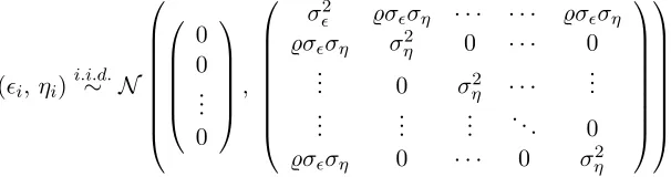
d= 400 and p = 400. A hundred sets ofi.i.d. (Y_i;X_i;Z_i;ǫ_i;η_i)n_i=1 are simulated where n is the sample size in each set and

(ǫi, ηi)i.i.d.∼ N

        

     

0 0 .. . 0

     ,

        

σ_ǫ2 ̺σǫση · · · ̺σǫση

̺σ_ǫσ_η σ2_η 0 · · · 0 ..

. 0 σ2_{η · · ·} ... ..

. ... ... . .. 0 ̺σǫση 0 · · · 0 σ2η

        

        

(39)

withσ2_ǫ := var(ǫi),σ2η := var(ηij) for allj, and̺the correlation betweenǫi andηij. We set̺= 0.05

to introduce endogeneity in all 400 components ofXi while ensuring the covariance matrix in (39)

generated by Matlab to be positive definite for the choices ofσ_ǫ and σ_η in Table 3.1 (larger values of ̺ fail to maintain the positive definiteness of (39)).

Table 3.1: Parameters for Designs A, B, C

Parameters Exp. 1 Exp. 2 Exp. 3 Exp. 4 Exp. 5

β∗

j(j= 1, ...,4) 0.5 0.5 0.25 0.5 0.5

σǫ 0.5 1 0.5 0.5 0.5

ση 0.5 1 0.5 0.5 0.5

n 399 399 399 200 800

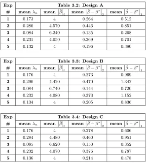
Three sparse designs are considered. In terms of the first-stage equations’ coefficients, for everyj andl= 5, ...,400, Design A setsπ_jl∗ = 0, Design B setsπ_jl∗ = 0_l.1, and Design C setsπ_jl∗ = 0.25l−3; for all three designs,π∗_jl= 0.5 for everyj and l= 1, ...,4. In terms of the main equation’s coefficients, for j = 5, ...,400, Design A sets β_j∗ = 0, Design B sets β_j∗ = 0_j.1, and Design C sets β_j∗ = 0.25j−3. For each sparse design, we perform five experiments differing in β∗_j (j = 1, ...,4), σ_ǫ, σ_η, and n. Table 3.1 summarizes the parameters for each of the five experiments.

For each simulation run h = 1, ...,100, we apply the modified algorithm in Section 2.2 with ς = ₂₅₆1 . For λ_n,js in (3), we apply (29)-(30) and iterate the “Adjusted-Penalization” step three times (i.e., a total of four iterations including the “Over-Penalization” step). With ˆση(4) from

the last iteration, we set ˆση := ˆσ(4)η , which is used in the modified algorithm for selecting λn in

step twice (i.e., a total of three iterations including the “Over-Penalization” step). Let λh_n denote the final second-stage regularization parameter and ˆβh the second-stage estimate for β∗ in the hth run. Tables 3.2-3.4 display the mean of λh_ns, ₁₀₀1 P100_h=1λh_n, the mean of the l₀₋norms of ˆβh,

1 100

P100

h=1P400j=11

n

ˆ

βh_{j 6}= 0o, the mean of the l2−errors, ₁₀₀1 P100h=1

βˆh₋β∗

2, as well as the mean of

thel1−errors, ₁₀₀1 P100h=1

βˆh₋β∗

1, for Designs A, B, and C, respectively.

The results show that our H2SLS in conjunction with themodified algorithm for settingλn and

λ_n,js perform well for these sparse designs. The directions and magnitudes of the changes in the results from Experiment 1 to another experiment agree with our predictions based on (37) and (28). For Design A (the exact sparsity case), the bound in (37) can be reduced toOκ−₂1√k2T0(1)

, a term that accounts for the estimation error; consequently, in view of (28), when the noise variance, ση,

is doubled, the means of theλh_ns and l₂₋errors are approximately doubled; when |β∗_|1 is changed from 2 to 1, the means of theλh_ns and l2−errors are also nearly halved; when the sample size nis

nearly doubled (halved), the means of theλh_ns andl2−errors are nearly decreased by a factor of√2

(respectively, increased by a factor of √2).

For the approximately sparse designs B and C, similar patterns are witnessed. The fact that thel2−errors of Design C are similar to those of Design B suggests that the actual approximation

errors are likely to be much smaller than the actual estimation errors. On the other hand, Design B yields the highest mean of the l1−errors, followed by Design C. In view of (38), this is because

B has the largestP400_j=5β_j∗among all three designs.

Exp Table 3.2: Design A

# meanλn mean

_βˆ

0 mean

_βˆ_−β∗

2 mean

_βˆ_−β∗

1

1 0.173 4 0.264 0.512

2 0.280 4.570 0.446 0.851

3 0.084 6.240 0.135 0.268

4 0.231 4.050 0.369 0.701

5 0.132 4 0.196 0.380

Exp Table 3.3: Design B

# meanλn mean

_βˆ

0 mean

_βˆ

−β

∗

2 mean

_βˆ

−β

∗

1

1 0.176 4 0.273 0.969

2 0.290 4.420 0.470 1.342

3 0.084 6.740 0.144 0.720

4 0.232 4.080 0.373 1.152

5 0.134 4 0.205 0.836

Exp Table 3.4: Design C

# meanλn mean

_βˆ

0 mean

_βˆ

−β

∗

2 mean

_βˆ

−β

∗

1

1 0.176 4 0.278 0.606

2 0.284 4.480 0.460 0.951

3 0.085 6.620 0.150 0.352

4 0.232 4.070 0.376 0.787

4

Future directions

This paper has explored the validity of the H2SLS estimation for linear triangular models where the number of endogenous regressors in the main equation and the number of instruments in the first-stage equations can exceed the sample size n, and the regression coefficients are sufficiently sparse. We establish finite-sample performance bounds and also provide a simple method for choosing the regularization parameter with asymptotic guarantees. The proposed procedure is tested on simulated data and the results show that our H2SLS in conjunction with the method for setting the regularization parameters perform well for various sparse designs.

There are two immediate extensions that worth exploring. First, as we have discussed in Section 2.2, selecting the constant C in (21) can be assisted with the CV criterion or the ESCV criterion proposed by Lim and Yu (2013). Here we lay out the details on how the ESCV criterion can be tailored to our “Adjusted-Penalization” step. Let the n observations be randomly assigned into T subsamples of size (n₋L), where L =_Tn. Suppose we consider a set of Cms (m = 1, ..., M) for the constant C in (21) and denote the resulting λn as λnm for each choice Cm. Givenλmn and

the subsample t, the “Adjusted-Penalization” step is performed to obtain ˆβ_t(λ_nm) and ˆY_t(λm_n) = ˆ

Xβˆt(λmn). For each m= 1, ..., M, following Lim and Yu (2013), we form

ES(λm_n) := Var( ˆd Y(λ

m n))

Y¯ˆ(λm

n)

2

n

= L n₋L

1 Z2_(λm

n)

with

d

Var( ˆY(λm_n)) := 1 T

T

X

t=1

Yˆt(λmn)−Y¯ˆ(λmn)

2_n,

Z2(λm_n) :=

¯ ˆ Y(λm_n)

q

n−L

L Var( ˆd Y(λmn))

,

¯ ˆ

Y(λm_n) := 1 T

T

X

t=1

ˆ Yt(λmn),

where we denote|a_|2_n:= _n1Pn_i=1a2_i. Let ˆσ_X∗ j =

q

1

n

Pn

i=1Xˆij2. We then apply their ESCV criterion:

Choose λm_n such that it minimizes ES(λm_n) over all m and Pp_j=1σˆX∗ j

βˆj(λmn)

is no greater than the one resulting from the optimal Cross-Validation (CV) choice. Lim and Yu (2013) recommend a grid-search algorithm to find a local minimum of ES as what is often done for the CV. Because the computational cost is rather high for our simulation exercise, we did not apply the ESCV criterion for selecting C in Section 3. However, it would be useful to evaluate the performance of this procedure with real data sets in the future.

techniques in our problem, albeit doing so would distract the main focus of this paper; therefore, we leave these extensions to future research.

Besides the above extensions, we discuss two important future directions beyond this research. One direction regards the high dimensional “control function” approach, which is a close alterna-tive to the H2SLS. Another direction regards inference strategies that can be built upon the H2SLS.

The “control function” approach. As an alternative to the ˆβH2SLS proposed in this paper,

an-other type of two-stage estimator based on the “control function” approach is worth being explored. The “control function” approach includes the first-stage estimation residuals ˆη_ij =X_{ij −}Z_ijˆπ_j as additional “control variables” (for the part of Xi that is correlated withǫi) in the regression ofYi

on Xi. In particular, we can perform the following estimation

ˆ

βHCF ∈argminβ,γ∈Rp 1

2n|Y −Xβ−ηγˆ |

2

2+λn(|β|1+|γ|1),

where the estimates ˆη = (X1−Z1πˆ1, ..., Xp−Zpπˆp) of η =

X1−Z1π1∗, ..., Xp−Zpπp∗

are ob-tained from (3).

When (1) and (2) are in the classical settings (fixedpandd), the two-stage least squares estima-tor is algebraically equivalent to a “control function” approach (e.g., Garen, 1984). Such algebraic equivalence no longer holds when regularization is introduced in the estimation. Nevertheless, the connection between ˆβH2SLS and ˆβHCF remains an interesting question for future research.

Inference based on H2SLS. Among existing literature, establishing variable selection consis-tency is the most popular approach to obtain inference results because it allows one to apply procedures from the classical low-dimensional regime by considering only the selected regressors. Variable selection consistency can be proved under a bounded “sparse eigenvalue condition” (e.g., Belloni and Chernozhukov, 2013) or an “incoherence” condition on the design matrix for the Lasso (e.g., Wainwright, 2009; Ravikumar, et al., 2010). The “incoherence condition” is a refined version of the “irrepresentable condition” by Zhao and Yu (2006) and the “neighborhood stability con-dition” by Meinshausen and Bühlmann (2006). Zhu (2013) establishes results regarding variable selection of ˆβ_H2SLS, which could be of independent interest1.

The drawback to the aforementioned post-variable-selection inference strategy is that the result-ing estimators suffer the problems arisresult-ing from the nonuniformity of limit theory (see, e.g., Leeb and Pötscher, 2006). Here we mean the nonuniformity inβ∗, the parameter vector of interest. Among recent development, several uniform inference strategies have been proposed (e.g., Javanmard and Montanari, 2014; van de Geer, Bühlmann, Ritov, and Dezeure, 2014; Zhang and Zhang, 2014). For the models of our interest, these inference strategies can be applied to construct confidence intervals for any coefficient in (1). In particular, these strategies rely on an initial estimator and in our case, such a candidate can be the ˆβ(2) in Theorem 2.2. To illustrate, we only sketch the strategy by Zhang and Zhang (2014) based on ˆβ(2) in the following.

Denote X_−j the columns ofX excluding the jth column. Following Zhang and Zhang (2014), forj_{∈ {}1, ..., p_}, we construct the following “de-biased” estimator,

˜

βj := ˆβ_j(2)+

r_jTY ₋Xβˆ(2) r_jTXj

(40)

1_{Note that in Zhu (2013), while the result establishesJ( ˆβ}

H2SLS) =J(β∗) with high probability for exactly sparse

β∗_{, the argument follows through if J(β}∗_{) is replaced with the thresholded subset S}

τ when β∗ is approximately

whererj = ˆXj−Xˆ−jθˆj with

ˆ

θj ∈arg min θj∈Rp−1

(

|Xˆj−Xˆ−jθj|22

2n +µn,j|θj|1

)

,

for a non-negative tuning parameterµn,j of order

q

logp

n . Note that (40) yields

√

nβ˜j −βj∗

=

1

√

nr T j ǫ

1

nrjTXj

−

1

√

n

P

l6=jrjTXl

ˆ

β_l(2)₋β_l∗

1

nrTjXj

. (41)

Moreover, we have

1 √_nX

l6=j

r_jTX_lβˆ_l(2)₋β_l∗

≤ max

l6=j

1

√_nhr_jTXˆl

+r_jTXl−Xˆli βˆ(2)−β∗

₁.

We can apply the argument in Zhang and Zhang (2014, Proposition 1) to show that

max

l6=j

1 n

r_jTXˆl

=Op

 

s

logp n

 .

By Lemma B.7 in this paper, we also have

1 nmaxl6=j

r_jTX_l−Xˆ_l=O_p(E)

where

E :=θˆj

1∨1

max

 

σX∗T1, ρX∗ρη s

logp n

  .

Note that, under the conditions in Theorem 2.2, if κ−₂1=O(1) and

|β_S∗c τ|1 =O



(_|β∗_|1∨1) (k_2∨1)

s

(k_1∨1) log(d_∨p) n

 ,

then we have

βˆ(2)₋β∗

1 =Op



(_|β∗_|1∨1) (k2∨1)

_(k

1∨1) log(d∨p)

n

1 2−ς

 .

Putting these facts together, if

√ n

 _{E ∨}

s

logp n



(_|β∗_|1∨1) (k2∨1)

_(k

1∨1) log(d∨p)

n

1 2−ς

=o(1),

then

1 √_nX

l6=j

rT_jXl

ˆ

Consequently, if 1_nrT_jXj →p D 6= 0, then √n

˜

βj −βˆj(2)

has the same asymptotic distribution as

the leading term D−1r T jǫ

√_n in (41).

Note that the de-biased estimator ˜β_j in (40) relies on ˆβ_j(2) whose construction uses ˆk₁ = maxj=1,...,p|J(ˆπj)|. To ensure ˆk1 ≥ k1 with probability at least 1 −o(1), we impose a

condi-tion on minl∈S_τj |π∗jl| in Lemma B.4. Under such a condition, the de-biased estimator discussed

above is valid uniformly inβ∗only but not in the nuisance parameters,π∗_js. Developing a de-biased H2SLS procedure that is valid uniformly in bothβ∗ andπ∗_js would be worth exploring in the future research.

A

Appendix: Main proofs

A.1 Proof for Theorem 2.1

Lemma A.1. Supposeλn satisfies that λn≥ T0 and the conditions in Lemmas A.3-A.4 hold. Let

b0 =κ2

˜

ρ4

X∗ κ2

2 ∨

1

. If

|β∗_|1λ−n1

_b

0logp

n ∨ T

2 1

≤c′′ (42)

for some universal constantc′′ >0, then there exist positive universal constants c∗₀,c∗₁ and c∗₂ such that, forτ = λn

κ₂ in (12), we have

|βˆH2SLS−β∗|2 ≤ c∗0

 λn√k2

κ₂ +

s

λ_n|β∗

Sc τ|1 κ₂

 := ¯B,

|βˆH2SLS−β∗|1 ≤ 4

p

k2B¯+|βS∗c τ|1

,

with probability at least 1−c∗₁exp(−c∗₂logp).

Proof. Let then_×p matrixη:= (η1, ..., ηn)T. We write

Y = Xβ∗+ǫ=X∗β∗+ (Xβ∗₋X∗β∗+ǫ) = X∗β∗+ (ηβ∗+ǫ)

= Xβˆ ∗+ (X∗₋Xˆ)β∗+ηβ∗+ǫ = Xβˆ ∗+ξ,

where

ξ:= (X∗₋Xˆ)β∗+ηβ∗+ǫ.

Let ˆv0 = ˆβ_{H2SLS −}β∗. Given a set S, recall that ˆv_{S ∈} p_×1 is the vector that has the same coordinates as ˆv on S and zero coordinates on the complement Sc of S. Define the Lagrangian L(β;λn) = ₂1_n|Y −Xβˆ |22+λn|β|₁. Since ˆβH2SLS is optimal, we have

L( ˆβH2SLS;λn)≤L(β∗;λn) =

1 2n|ξ|

2